Article

Atmospheric PM2.5 Prediction Based on Multiple Model Adaptive Unscented Kalman Filter

1
Faculty of Information Technology, Beijing University of Technology, Beijing 100124, China
2
Beijing Key Laboratory of Computational Intelligence and Intelligent System, Engineering Research Center of Digital Community, Ministry of Education, Beijing 100124, China
3
School of Information Engineering, Inner Mongolia University of Science and Technology, Baotou 014010, China
*
Author to whom correspondence should be addressed.
Atmosphere 2021, 12(5), 607; https://doi.org/10.3390/atmos12050607
Submission received: 4 March 2021 / Revised: 21 April 2021 / Accepted: 29 April 2021 / Published: 7 May 2021
(This article belongs to the Special Issue Efficiency Evaluation in Atmospheric Environment)

Abstract

:
The PM 2.5 concentration model is the key to predict PM 2.5 concentration. During the prediction of atmospheric PM 2.5 concentration based on prediction model, the prediction model of PM 2.5 concentration cannot be usually accurately described. For the PM 2.5 concentration model in the same period, the dynamic characteristics of the model will change under the influence of many factors. Similarly, for different time periods, the corresponding models of PM 2.5 concentration may be different, and the single model cannot play the corresponding ability to predict PM 2.5 concentration. The single model leads to the decline of prediction accuracy. To improve the accuracy of PM 2.5 concentration prediction in this solution, a multiple model adaptive unscented Kalman filter (MMAUKF) method is proposed in this paper. Firstly, the PM 2.5 concentration data in three time periods of the day are taken as the research object, the nonlinear state space model frame of a support vector regression (SVR) method is established. Secondly, the frame of the SVR model in three time periods is combined with an adaptive unscented Kalman filter (AUKF) to predict PM 2.5 concentration in the next hour, respectively. Then, the predicted value of three time periods is fused into the final predicted PM 2.5 concentration by Bayesian weighting method. Finally, the proposed method is compared with the single support vector regression-adaptive unscented Kalman filter (SVR-AUKF), autoregressive model-Kalman (AR-Kalman), autoregressive model (AR) and back propagation neural network (BP). The prediction results show that the accuracy of PM 2.5 concentration prediction is improved in whole time period.

1. Introduction

In recent years, the global economic integration has developed rapidly. The Beijing–Tianjin–Hebei region economic belt (Beijing–Tianjin–Hebei) as the development area has gradually been formed. The severe haze event happened in Beijing in 2013 [1]. The fine particle matter (PM 2.5 ) is a particle with a diameter of 2.5 μ or less in the atmosphere. PM 2.5 has a long atmospheric residence time, it has an important impact on environmental quality, atmospheric visibility, human health and climate change. PM 2.5 has become the primary air pollutant in China. It mainly contains polycyclic aromatic hydrocarbons and heavy metals [2]. The harmful substances mainly including heavy metals, microorganisms and organic volatile compounds [3]. The human respiratory system is damaged by these harmful substances, which leads to damage to human health and death [4]. The government has also formulated a large number of policies, and a large number of software and automatic monitoring equipment are installed throughout every corner of the city. Once PM 2.5 concentration monitored exceeds the specified range, the environmental supervision department will send effective information to inform people to reduce social activities to avoid long-term exposure to the environment with high PM 2.5 concentration [5].
The PM 2.5 prediction method can be usually divided into physical and chemical methods and statistical methods [6]. Physical and chemical reaction methods do not need a large number of historical meteorological data. The chemical reactions of exhaust gas from pollution sources, emissions and fuel energy consumption need to have a deterministic description source. For example, Sun et al. proposed a cuckoo search algorithm based on principal component analysis and least squares support vector machine (PCA-LSSVM) to predict PM 2.5 concentration [7]. Zhang et al. observed the pollution characteristics of PM 2.5 and PM 1 in autumn in Beijing and identified the source regions of PM 2.5 and PM 1 by the positive matrix decomposition (PMF), the backward trajectory and potential source contribution function (PSCF) model [8].
On the other hand, the statistical methods are gradually applied in the field of artificial intelligence. Some statistical method-based AIs have been adopted. For example, for regression model, neural network, machine learning algorithm, time series method and Kalman filter, the relationship of pollutants and prediction variables are established by different functions or network models. Coburn W. G. et al. proposed an enhanced PM 2.5 air quality prediction model based on nonlinear regression (NLR) and reverse trajectory concentration to predict PM 2.5 in Louisville metropolitan area, Kentucky [9]. Elangasinghe, M.A. et al. analyzed the PM 10 and PM 2.5 concentration time series by artificial neural network and K-means clustering [10,11]. For this method, the artificial neural network (ANN) model is used, and it has better performance in picking up high concentrations. The artificial neural network sometimes falls into the problem of local over fitting; but, the neural network model needs a lot of historical data for training, which increases the complexity and time of calculation. Zhou et al. proposed an ensemble empirical model decomposition generalized regression neural network (EEMD-GRNN) model to predict PM 2.5 concentration in a day [12]. The EEMD method is used to determine different information scales in the original time series for this method. In addition, each decomposed IMF has similar frequency characteristics. Thus, the efficiency and accuracy of prediction is improved. There are many other experts who are beginning to focus on application of artificial intelligence algorithm to propose the corresponding algorithm to predict PM 2.5 . For example, Zhan et al. studied the spatial and temporal daily PM 2.5 concentration prediction based on spatial explicit machine learning algorithm [13]. In this study, geographically weighted gradient boosting machine (GW-GBM) method is proposed. The deviation of PM 2.5 concentration estimation is overcome, so that the prediction is more accurate. Some other scholars use time series method to predict the PM 2.5 concentration [14,15,16,17,18]. For example, Akhil Kadiyala used a vector time series and back propagation neural network (VTS-BPNN) method to review articles of hybrid indoor air quality (IAQ) models. In dynamic atmosphere, it is sometimes impossible to measure every variable. The Kalman filter can estimate the missing information by the limited, indirect and noisy measurement information, which has the characteristics of small data storage and handling multidimensional and non-stationary random processes. The Kalman filtering is also used to predict the future trend of dynamic system [19]. For example, Federico Cassola used a Kalman filter to forecast weather by 2-year-long data sets. The traditional Kalman filtering method is only suitable for linear system, and the observation equation must also be linear. The nonlinear Kalman filters are applied to deal with the estimation of nonlinear systems [20,21,22,23,24,25]. However, the extended Kalman filter (EKF) method needs to linearize the nonlinear function with the first or second order term of Taylor formula, and the Jacobian matrix is calculated. The PM 2.5 concentration prediction is not very accurate by the EKF method. To solve this problem, the unscented Kalman filter (UKF) method is applied to predict the future trend.
The appeal method is used to predict PM 2.5 concentration by a single model. In practice, the PM 2.5 concentration is always changing in different environments or time periods. A single model can usually predict the PM 2.5 concentration in the current situation. Once the original environment changes, the original model will not match the new environment, and the prediction error will be generated. Thus, it is the main problem to establish the corresponding prediction model for different states. Blom, H.A.P. et al. have proposed a multiple model theory [26]. For example, the problem of outlet temperature of flow pressure controlled tubular heat exchanger is studied [27]. This method is based on the linear generalized predictive control (LGPC). The main idea of the strategy uses multiple linear models to represent the operating environment of multiple systems. Each system is accurately identified by the intelligent decision mechanism (IDM) at every moment, the target can be controlled more accurately. In addition, Xie et al. have proposed a comprehensive vehicle trajectory prediction method based on the combination of physics and mobility [28]. An interactive multiple model prediction method based on the two prediction models is proposed, which realizes recursive adjustment and switching by the probability of each model occurrence, and the lane change is analyzed to realize vehicle trajectory. Li et al. used multiple model theory to control variables under different working conditions or different states to improve control accuracy [29,30,31,32]. Although the idea of multiple models is widely applied in the field of control, it has not been applied to the prediction field of atmospheric PM 2.5 concentration.
To predict PM 2.5 concentration more accurately, the idea of multiple model is introduced into the atmosphere prediction, and a multiple model adaptive unscented Kalman filter method is proposed to predict PM 2.5 concentration in the next hour. The contributions of this paper are given as follows:
(1)
The PM 2.5 concentration prediction values of different time periods are fused to predict the change trend and fluctuation of PM 2.5 concentration by the multiple model adaptive method.
(2)
The proposed MMAUKF method also considers the estimation of noise in the prediction process. When the PM 2.5 concentration is predicted, the noise is also estimated adaptively by estimator.
(3)
The proposed MMAUKF method improves the accuracy and stability of PM 2.5 concentration prediction.
The remaining sections of the paper are described as follows. Section 2 introduces the establishment of PM 2.5 concentration prediction system. Section 3 mainly describes PM 2.5 concentration prediction based on SVR-AUKF method. Section 4 is a multiple model adaptive unscented Kalman filter for PM 2.5 concentration prediction. Section 5 is the simulation results. Section 6 is the conclusion of this paper.

2. The Establishment of PM 2.5 Concentration Prediction System

Most scholars pay attention to the prediction of PM 2.5 concentration. A large number of atmospheric PM 2.5 monitoring points are established in the city. In this paper, a monitoring point of a campus in the Chaoyang District of Beijing is taken as the research area, and the monitoring of PM 2.5 concentration on campus is provided 24 h a day. The PM 2.5 concentration is predicted by monitoring the historical atmospheric meteorological data monitoring platform. The data monitoring platform is composed of an outdoor air sensor probe, upper computer and solar power supply system. The measurement error of the monitoring probe is less than 0.05%, which has a stable operating environment and avoids the interference of the external environment. The monitor can directly access the monitored data by the network cloud. The power supply system of the equipment is a stable power supply system, which is provided by the renewable energy solar panel for the real-time and stable operation. The data monitoring platform is shown in Figure 1.
The simulation experimental data are obtained by this platform in this section. The main monitoring data of the atmospheric monitoring platform include PM 2.5 , PM 10 , SO 2 , NO 2 , CO, O 3 , humidity (RH), temperature (T) and air quality index (AQI). The historical data of PM 2.5 concentration in July 2018 are used as the study object in this paper. The relationship between PM 2.5 concentration and other potential variables was illustrated by the scatter plot of PM 2.5 concentration in Figure 2 (the blue points represent PM 2.5 and other air pollutants, the green points represent PM 2.5 and meteorological conditions).
The mean and variance of pollutants and meteorological conditions are given by statistical methods in Table 1. The mean represents the mean of time series, and standard deviation represent the mean change of the time series of the monitored data.
According to the analysis of literature [12], the PM 2.5 concentration is closely related to other monitoring variables, the monitored variables (PM 2.5 , PM 10 , SO 2 , NO 2 , CO, O 3 , humidity (RH), temperature (T)) are used as the input variables of the SVR model, and PM 2.5 concentration is used as the output variables of the model. To improve the accuracy of the proposed method in predicting PM 2.5 concentration, the prediction accuracy of the proposed method is compare with the other single model method by three error indexes. The three error statistics methods are given as follows:
M A E = 1 n k = 1 n | y k + 1 y ^ k + 1 |
M A P E = 1 n k = 1 n | y k + 1 y ^ k + 1 y k + 1 | × 100 %
R M S E = 1 n k = 1 n ( y k + 1 y ^ k + 1 ) 2
where y k + 1 represents the actual PM 2.5 concentration value, y ^ k + 1 is PM 2.5 concentration prediction value at time k + 1 , ( k = 0 , 1 , , n ) , n is the number points in the test dataset. The MAE is mean absolute error. The MAPE is mean absolute percentage error. The RMSE denotes root mean square error. These performance indexes analyze the error between the predicted value and the actual value, and compare the prediction of PM 2.5 concentration by different methods.

3. PM 2.5 Concentration Prediction Based on the SVR-AUKF Method

3.1. Support Vector Regression

In this section, the state space equation framework based on SVR is introduced. The state equation framework is combined with adaptive Kalman filter to achieve state regression and adaptive noise estimation. The support vector machine (SVM) is a theoretical method of pattern recognition, which is usually used for classification and regression [33,34,35]. The artificial intelligence is developed rapidly, the regression problem is also widely used. The SVR is one of the emerging methods [36]. In the regression problem, the correlation function is establish between input variables and output variables. The SVR method mainly constructs linear decision function in high-dimensional space to realize model prediction. In SVR, a set of training samples { x i , y i }, ( i = 1 , 2 , , n ) is usually given. The sample regression function is described as follows:
f ( x ) = w , x + b
where w is the regression coefficient, and b is bias. , represents the dot product, which can be solved by convex optimization problems [37]. When the f exists and approximates ( x i , y i ) , the errors are allowed. The slack variables ξ , ξ i * is introduced to cope with infeasible constraints of the optimization problem. The formula is shown as follows:
m i n 1 2 w 2 + C i = 1 N ( ξ i + ξ i * )
s . t . y i w , x b ε + ξ i y i + w , x + b ε + ξ i * ξ i , ξ i * 0
where C is trade off parameter between f and larger than ε , ε is the tolerance coefficient. The dual optimization problem is obtained by using Lagrange multipliers, which is described as follows:
M a x 1 2 i = 1 , j = 1 N ( α j α i * ) ( α j α j * ) K ( x i , x j ) i = 1 N ( α i + α i * ) ε + i = 1 N ( α i α i * ) y i
where α i , α i * is Lagrange multipliers, K ( x i , x j ) represents kernel function. i = 1 N y i ( α i α i * ) = 0 is constraint condition. 0 < α i , α i * < C . The regression function equation can be obtained as follows:
f ( x ) = i = 1 N ( α i α i * ) K ( x , x i * ) + b
where w , x can be obtained as follows:
w , x = i N ( α i α i * ) x i
K ( x , x i ) = e x p ( x i x j 2 σ 2 )
where σ is the radial basis function (RBF) width. The b is calculated by Karush–Kuhn–Tucker (KKT) conditions [37]. In this paper, the optimal choice of C and σ are respectively 2 5 and 0.0825 by multi-fold cross-validation.
b = y i w , x i ε , 0 < α i < C
b = y i w , x i + ε , 0 < α i * < C
When the PM 2.5 concentration is predicted, the environment is always complex and changeable. There are always various external noises, uncertainties and randomness, which results in the prediction accuracy deviation [38]. In this paper, the unscented Kalman filter (UKF) method is introduced to deal with the uncertainty and randomness by constantly updating the status.

3.2. Unscented Kalman Filter Method

The traditional KF method often loses its optimality [39]. The UKF is introduced in this section. The UKF method is based on UT transform and adopts Kalman linear filter framework. The SVR-UKF is used in this paper. The nonlinear state equation frame of SVR method is given as follows:
x k + 1 = f ( x k ) + w k
y k = h ( x k ) + v k
where f and h are the nonlinear equation and observation function, respectively. w k and v k are the Gaussian white noise of x k and y k , respectively. q and r are the mean values of w k and v k , respectively. Q and R are covariance matrices of w k and v k , respectively. Assuming nonlinear change y = f ( x ) , the state vector is an n dimensional random variable. The x ¯ is mean value, and the P is variance. x k denotes the state vector of PM 2.5 concentration. y k represents the observation vector of PM 2.5 concentration. The n is state dimension. The initial value of the filter is calculated as follows:
x ¯ 0 = E ( x 0 )
P 0 = E [ ( x 0 x ¯ 0 ) ( x 0 x ¯ 0 ) T ]
where E is expected average, x ¯ 0 is mean value, P 0 is covariance. The derivation process of UKF is given in [38]. The final derivation result of UKF is given directly in this paper. The x ^ k + 1 | k is given as follows:
x ^ k + 1 | k = i = 0 2 n ω ( i ) x k + 1 | k ( i ) + q k
where ω is a non-negative weight coefficient. The covariance matrix is calculated as follows:
P k + 1 | k = i = 0 2 n ω ( i ) [ x ^ k + 1 | k x k + 1 | k ( i ) ] [ x ^ k + 1 | k x k + 1 | k ( i ) ] T + Q k
The predicted observation value is obtained as follows:
y k + 1 | k ( i ) = h [ x k + 1 | k ( i ) ]
The predicted mean and covariance of the system are described by weighted sum as follows:
y ¯ k + 1 | k = i = 0 2 n ω ( i ) y k + 1 | k ( i ) + r k
The Kalman gain is calculated as follows:
K k + 1 = P x k y k P y k y k 1
where P y k y k , P x k y k is calculated separately as follows:
P y k y k = i = 0 2 n ω ( i ) [ y k + 1 | k ( i ) y ¯ k + 1 | k ) ] [ y k + 1 | k ( i ) y ¯ k + 1 | k ] T + R k
P x k y k = i = 0 2 n ω ( i ) [ x k + 1 | k ( i ) y ¯ k + 1 | k ] [ x k + 1 | k ( i ) y ¯ k + 1 | k ] T
The state update is calculated as follows:
x ^ k + 1 | k + 1 = x ^ k + 1 | k + K k + 1 [ y k + 1 y ^ k + 1 | k ]
The covariance update is calculated as follows:
P k + 1 | k + 1 = P k + 1 | k K k + 1 P y k y k K k + 1 T
For PM 2.5 concentration prediction problems, statistical characteristics of interference signals are always not known. To solve the influence of noise on PM 2.5 concentration prediction, the AUKF method is used to estimate the noise in the next section.

3.3. Adaptive Unscented Kalman Filter Noise Estimation for PM 2.5 Concentration Prediction

When the statistical characteristics of the prior noise are given, the SVR-UKF prediction accuracy is usually accurate [37]. In complex atmospheric environments, the PM 2.5 concentration prediction is accompanied by various kinds of noise, and the process noise ( q k , Q k ) and the measurement noise covariance ( r k , R k ) are usually unknown or incorrect, which affects accuracy of prediction. The AUKF method is used to estimate noise adaptively and effectively avoid the deviation caused by noise in this paper. The Figure 3 shows the schematic diagram of the SVR-AUKF PM 2.5 concentration prediction method.
The noise estimation formula is given as follows. The mean value of process noise is given as follows:
q ^ k + 1 = ( 1 d k + 1 ) q ^ k + d k + 1 [ x ^ k | k i = 0 2 n ω i ( m ) f ( x ( i ) ( k ) ) ]
where d k + 1 is obtained as follows:
d k + 1 = 1 b 1 b k + 1
where b is the forgetting factor, which is set as 0.98 in this paper. The process noise covariance is estimated as follows:
Q ^ k + 1 = ( 1 d k + 1 ) Q ^ k + d k + 1 [ K k + 1 F k + 1 F k T K k + 1 + P k + 1 | k + 1 i = 0 2 n ω ( i ) ( m ) ( x k + 1 | k ( i ) x ^ k + 1 | k ) ( x k + 1 | k ( i ) x ^ k + 1 | k ) T ]
where F k + 1 is obtained as follows:
F k + 1 = y k + 1 y ^ k + 1
The mean value of measured noise is estimated as follows:
r ^ k + 1 = ( 1 d k + 1 ) r ^ k + d k + 1 [ y k + 1 i = 0 2 n ω i ( m ) h ( x k + 1 | k ( i ) ) ]
The measurement noise covariance is estimated as follows:
R ^ k + 1 = ( 1 d k + 1 ) R ^ k + d k + 1 [ F k + 1 F k + 1 T i = 0 2 n ω i ( c ) ( y k + 1 | k ( i ) y ¯ k + 1 | k ) ( y k + 1 | k ( i ) y ¯ k + 1 | k ) T ]
The SVR-AUKF method has been given in this section. The PM 2.5 concentration is predicted based on the SVR-AUKF method, and the prediction result of this method is shown as follows:
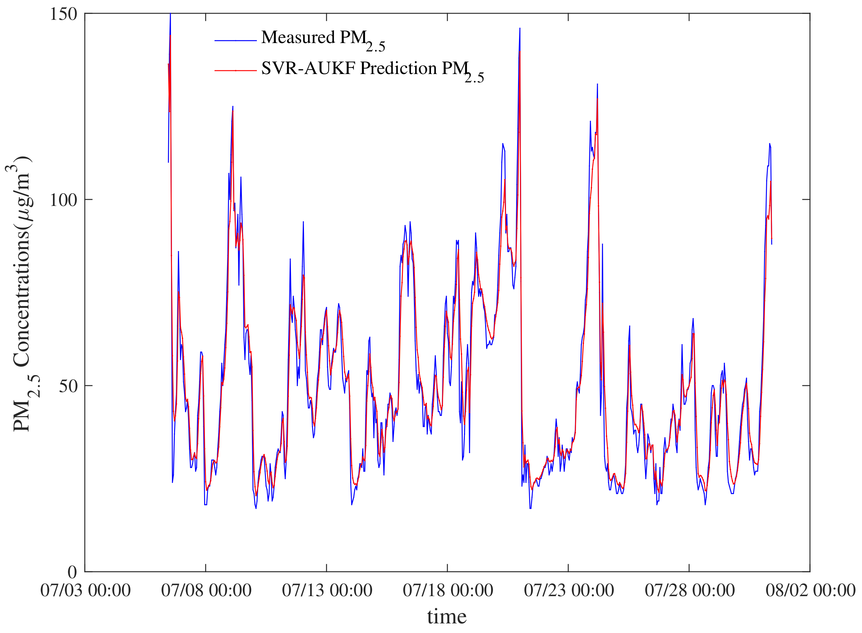
It can be seen from Figure 4 that the curve of PM 2.5 concentration predicted by single model SVR-AUKF method is basically consistent with the curve of actual measured value. There will be large error at some individual time points. The concentration of PM 2.5 also changed in different time periods. The single model SVR-AUKF method can not fully reflect the change of PM 2.5 concentration in the whole process and then produce errors. In order to fully reflect the change of PM 2.5 concentration, the multiple model prediction method is introduced to improve the prediction accuracy of PM 2.5 concentration and reduce error. The PM 2.5 concentration prediction of multiple model adaptive unscented Kalman filter is described in the next section.

4. Multiple Model Adaptive Unscented Kalman Filter for PM 2.5 Concentration Prediction

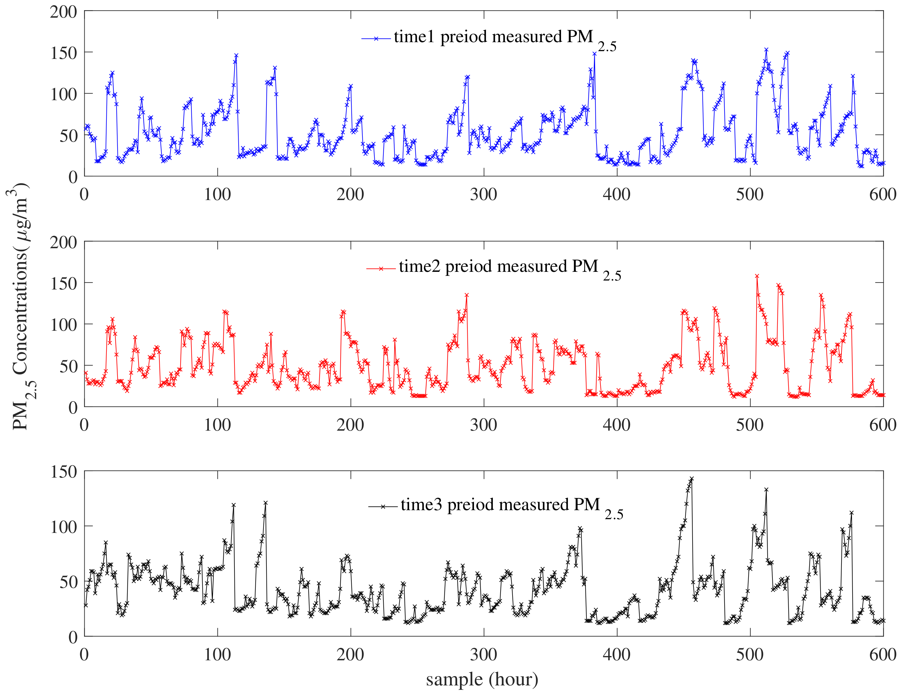
In the process of predicting PM 2.5 concentration, the single model is often not accurate enough, because the dynamic characteristics of the model will be affected by a variety of variables in different time periods. According to the reference [40], even in the same day, the pollutants will fluctuate greatly in different time periods. The model will also be affected. To predict PM 2.5 concentration more accurately in different time periods, the MMAUKF method is proposed. Due to the change of temperature and humidity in the morning, middle and evening, the concentration of PM 2.5 also changes, the typical time of the day is mainly in the morning, noon and evening. The three representative time periods are selected as the research object. The predicted PM 2.5 concentration data are divided into three time periods, which are 23:00~6:00, 7:00~14:00, 15:00~22:00, respectively. The PM 2.5 concentration model is established based on the data of different time periods. The PM 2.5 concentration data in different time periods are shown in Figure 5.
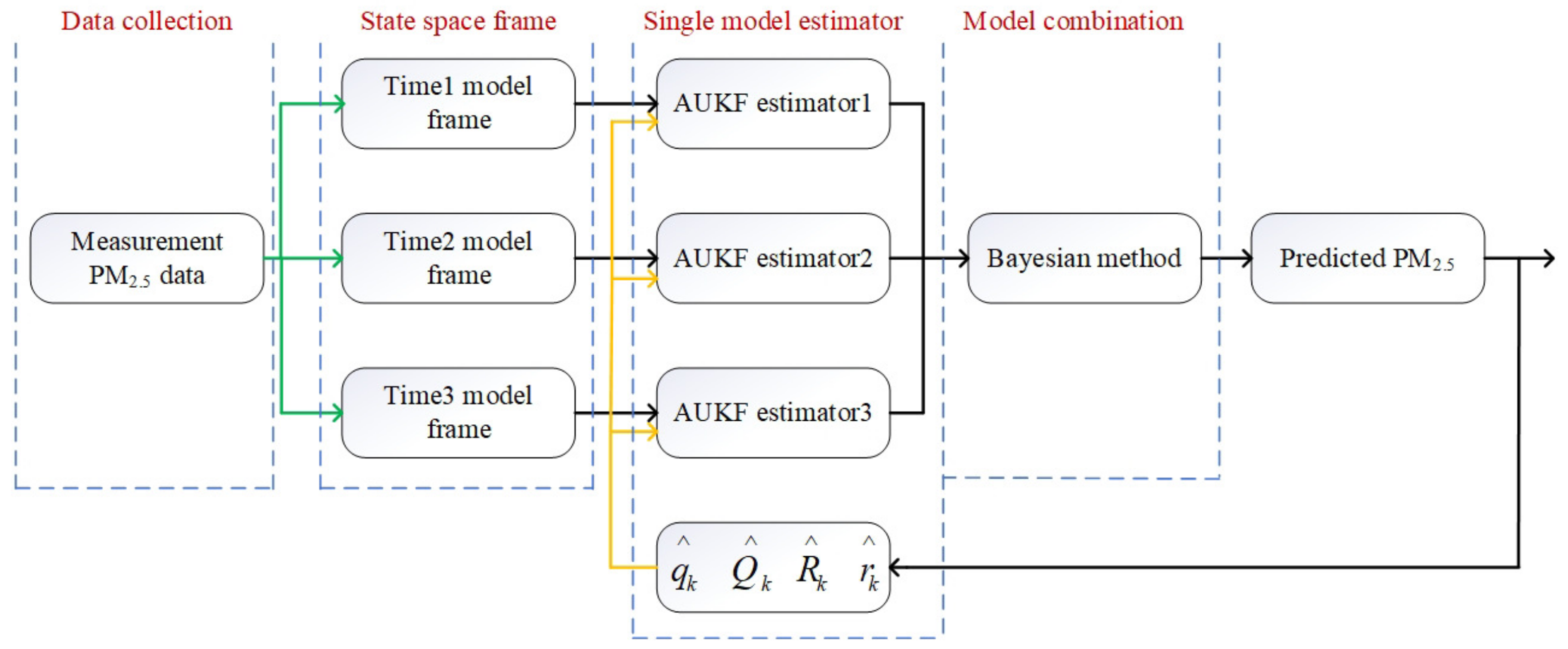
The obtained PM 2.5 concentration prediction values from different time periods are fused by Bayesian method. The proposed MMAUKF method is implemented to predict PM 2.5 concentration. The structure chart of MMAUKF method is shown as follows:
As shown in Figure 6, the structure chart of MMAUKF method for PM 2.5 prediction concentration based on SVR-AUKF method is given. The final predicted value is obtained by weighting. The feedback of each adaptive Kalman filter total output is used as the initial value for predicting the next moment. When the MMAUKF method is used to predict PM 2.5 concentration, the weight value calculation is the key to solving the PM 2.5 concentration prediction. The weight value is determined by the probability of selected model in the current period. The prediction error reflects the accuracy of the method. The error is small, which indicates the prediction accuracy of the selected model is high, and the probability of the selected model is high. The final fusion PM 2.5 concentration value is obtained by Bayesian method.
In this section, the Bayesian theory is adopted to predict PM 2.5 . The y ^ 1 , y ^ 2 and y ^ 3 are obtained for PM 2.5 concentration prediction value at the corresponding time period. When the predicted value is close to the measured value in the current time period, the weight value is lager. The predicted values in three time periods are calculated as follows:
y ^ k + 1 = W 1 · y ^ 1 , k + 1 + W 2 · y ^ 2 , k + 1 + W 3 · y ^ 3 , k + 1
where W is the weight values. The weighted sum is given as follows:
W 1 + W 2 + W 3 = 1
The prediction error ε is given as follows:
ε i , k + 1 = y i , k + 1 y ^ i , k + 1
where y i , k + 1 is the measured PM 2.5 concentration value, ( i = 0 , 1 , 2 , , n ) . y ^ i , k + 1 is the estimated PM 2.5 concentration value. k is the sampling period. Thus, the weight or the probability of selected model are given as follows: the initial values probability of the ith model are equal for each time period. The initial values are calculated as follows:
P ( M i | y ( 0 ) ) = 1 / M i
The conditional probability density function of the measured value is obtained as follows:
f ( y i , k + 1 | M i ) = 1 ( 2 π ) m / 2 Q i , k + 1 1 / 2 e x p ( 1 2 ε i , k + 1 T Q i , k + 1 1 ( k ) ε i , k + 1 )
where M i represents the parameter set of the ith ( i = 1 , 2 , 3 ) model. m is the number of measurement value, m = 1 . Q i , k represents the process noise variance corresponding to the ith filter estimator.
W j = P ( M j | y i , k + 1 ) = f ( y i , k + 1 | M i ) P ( M j ) i = 1 3 f ( y i , k + 1 | M i ) P ( M i )
The conditional probability density of the measured values of each time period model according to Bayesian theory is calculated as follows:
P ( M i | y i , k ) = P ( y i , k | M i ) P ( M i ) P ( y i , k )
where P ( y i , k | M i ) = P ( y i , k ) . The formula (36) is deduced as follows:
W j , k + 1 = P ( M j | y i , k + 1 ) = f ( y i , k + 1 | M i ) P ( M j | y i , k ) i = 1 3 f ( y i , k + 1 | M i ) P ( M j | y i , k )
where j is observer number. According to the above formula, the weight is calculated in three different time periods for PM 2.5 concentration prediction, and the fusion prediction result is obtained by formula (31).

5. The Simulation Results

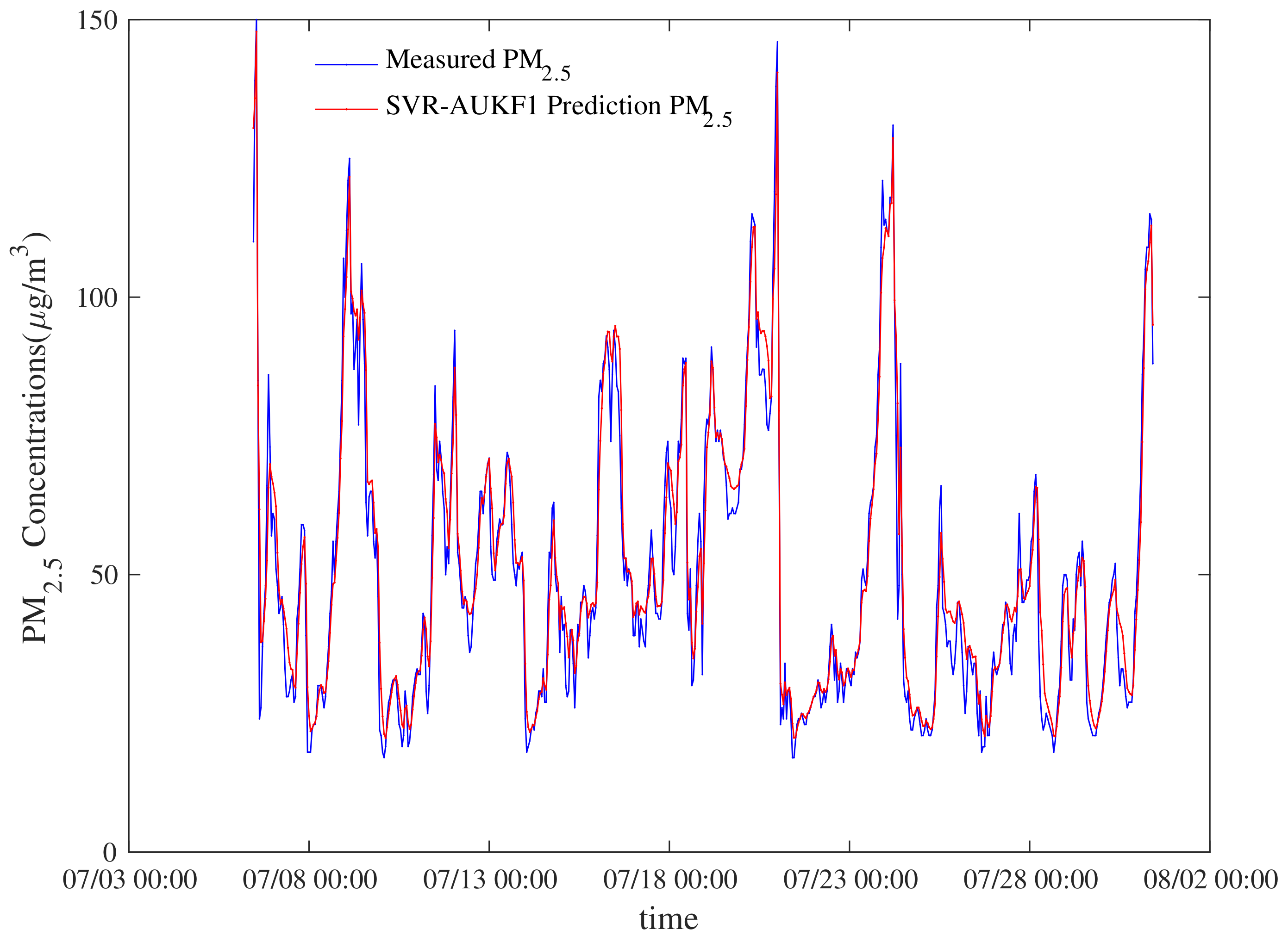
In this section, the prediction results of different methods are described, and the performance indexes of the error are given. In order to verify the accuracy of the proposed method, the three time periods of PM 2.5 concentration are predicted, and the PM 2.5 concentration of the whole time period is predicted by the proposed method. Through the comparison of different methods, a more accurate prediction method is shown. The predicted PM 2.5 concentration value by SVR-AUKF1 is given in Figure 7.
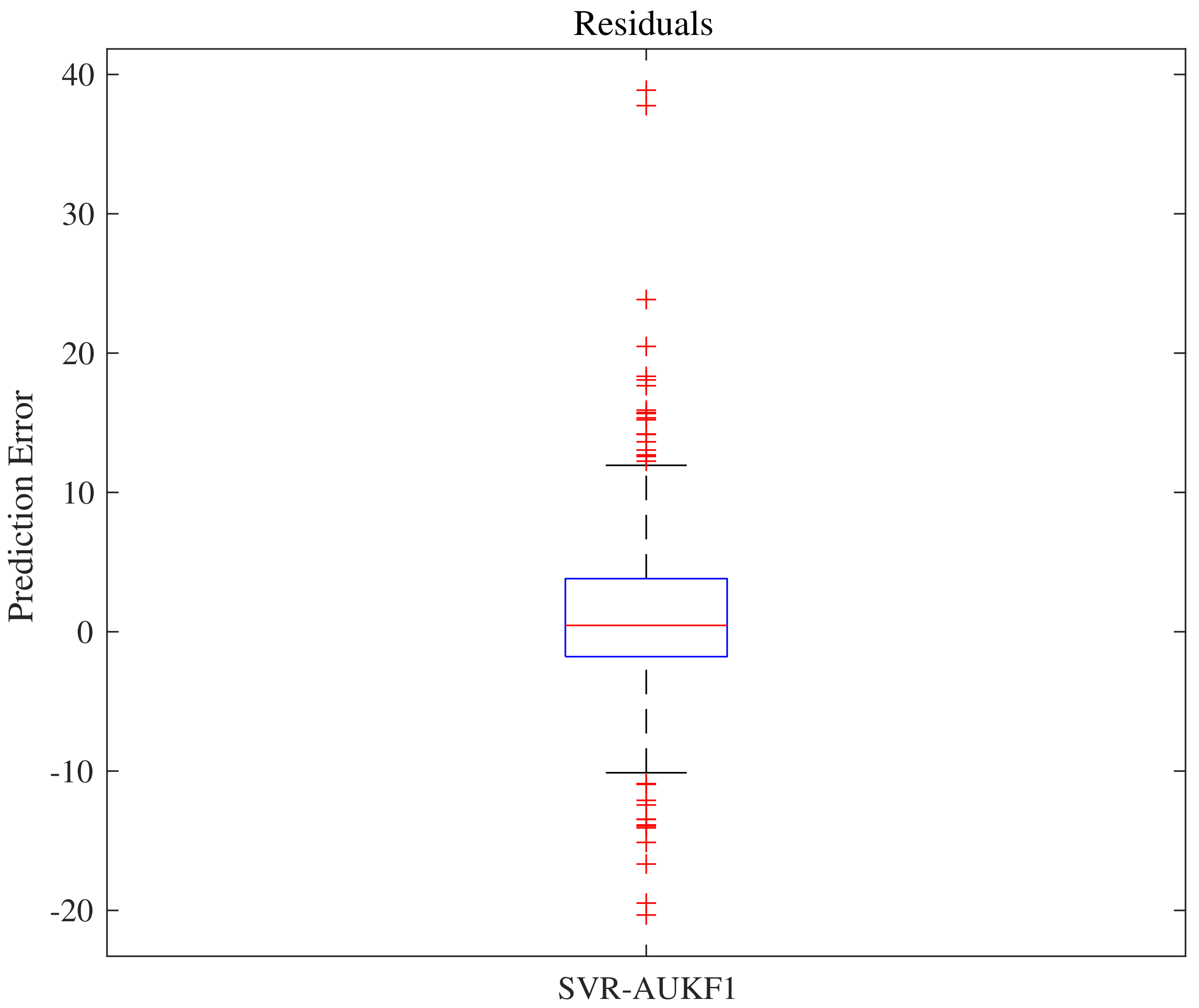
The prediction residuals of SVR-AUKF1 are shown in Figure 8.
For further simulation, this paper assumes that the unknown noise is Gaussian white noise. According to the actual PM 2.5 concentration in three time periods, the initial states x 1 , ( 0 ) = 120 , x 2 , ( 0 ) = 58 and x 3 , ( 0 ) = 78 are given, respectively. Figure 7 shows the PM 2.5 concentration prediction of SVR-AUKF1. It can be seen that there are still some errors for the whole sampling period in Figure 7. The MAE is 4.1994, the MAPE is 9.6523 and the RMSE is 6.2302. When the prediction is relatively accurate at the beginning of the time period. The errors will be produced in some point of time period. The SVR-AUKF1 method cannot predict PM 2.5 concentration accurately in the whole time period. The predicted PM 2.5 concentration value by SVR-AUKF2 is given in Figure 9.
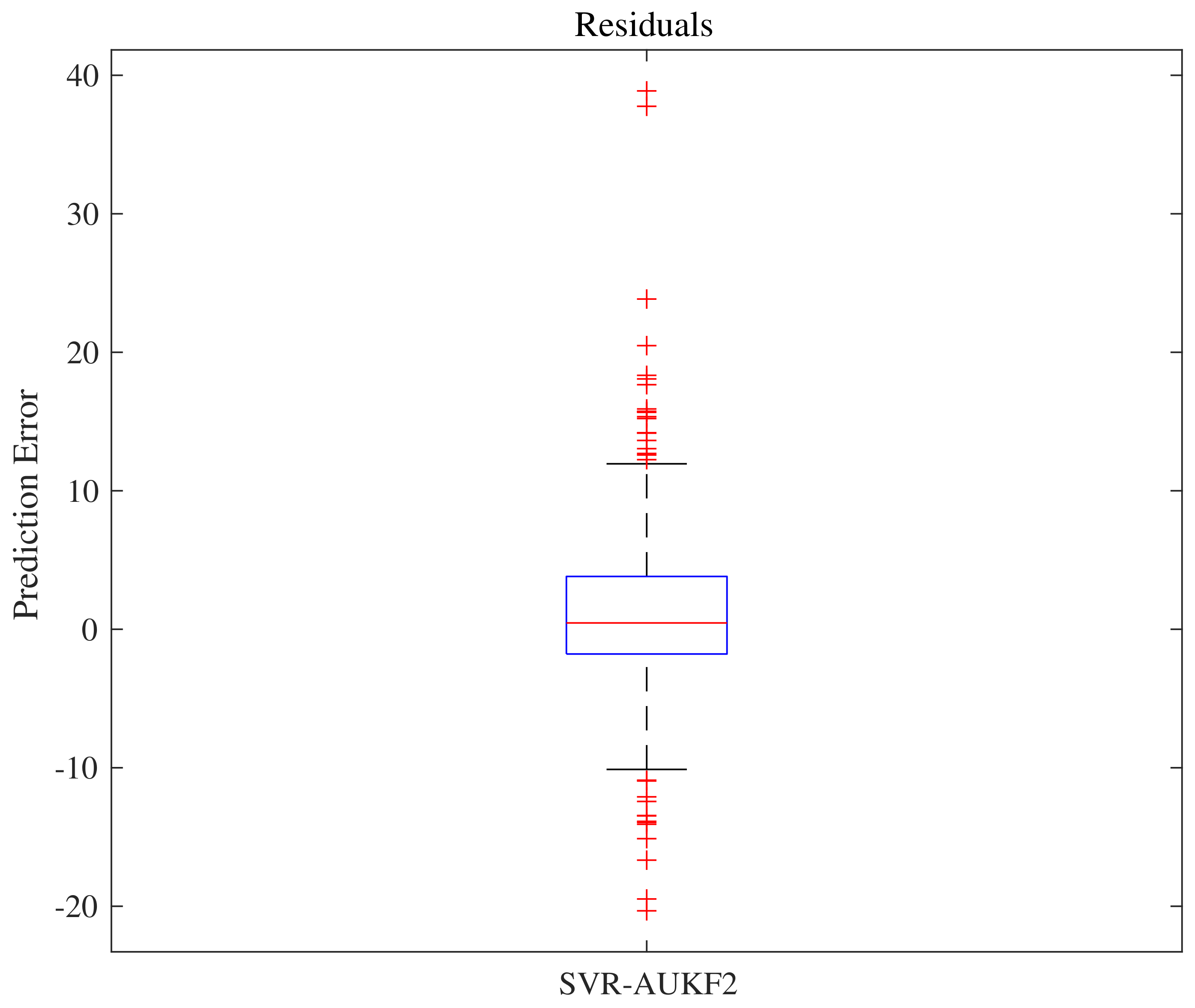
The prediction residuals of SVR-AUKF2 are shown in Figure 10.
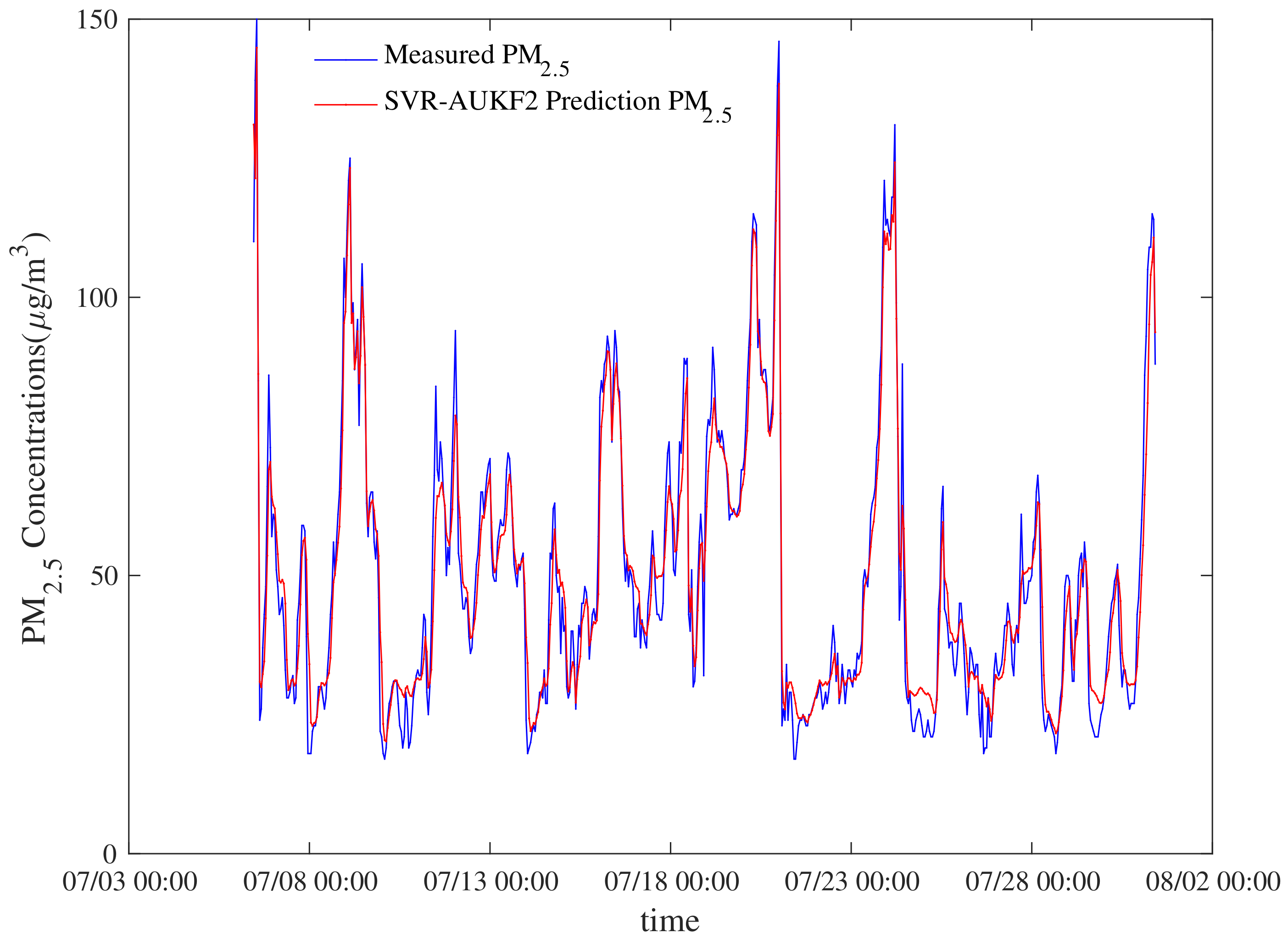
Figure 9 shows the predicted PM 2.5 concentration based on SVR-AUKF2 method. The prediction value is closer to the measured PM 2.5 concentration in the time range of (07/08 00:00∼07/13 00:00). The MAE is 4.3706, the MAPE is 10.7784 and the RMSE is 5.9424. Although the single model can accurately predict the PM 2.5 concentration in the current time period, the model will be affected by the environmental changes in different periods, which will affect the accuracy of PM 2.5 concentration prediction. The predicted PM 2.5 concentration value by SVR-AUKF3 is given in Figure 11.
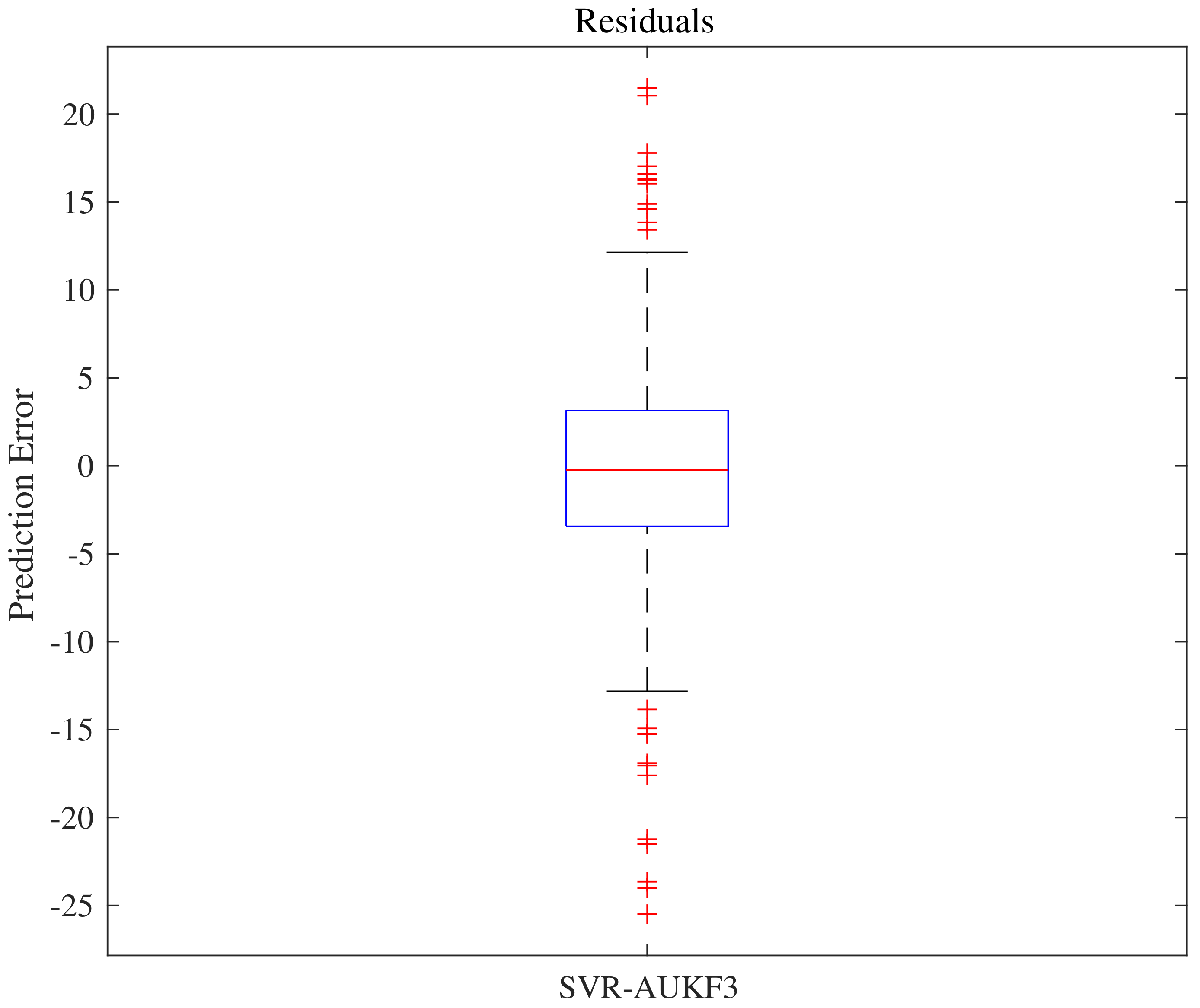
The prediction residuals of SVR-AUKF3 are shown in Figure 12.
The Figure 11 shows the predicted PM 2.5 concentration value based on the SVR-AUKF3 method. The prediction value is close to the measured value in the time range of (07/13 00:00∼07/18 00:00). The MAE is 4.4815 the MAPE is 11.8585 and the RMSE is 6.2018. In other time periods, the prediction accuracy of individual points can still be improved. In order to further improve the prediction accuracy, the multiple model method should be used to predict PM 2.5 concentration in different time periods.
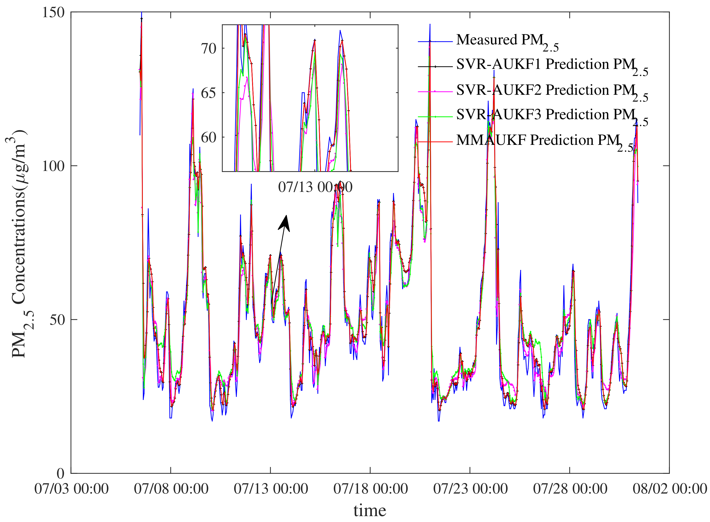
The proposed MMAUKF method is compared with SVR-AUKF1, SVR-AUKF2 and SVR-AUKF3 methods in Figure 13.
The statistical errors based on SVR-AUKF methods for PM 2.5 concentration in three time periods are shown in Table 2.
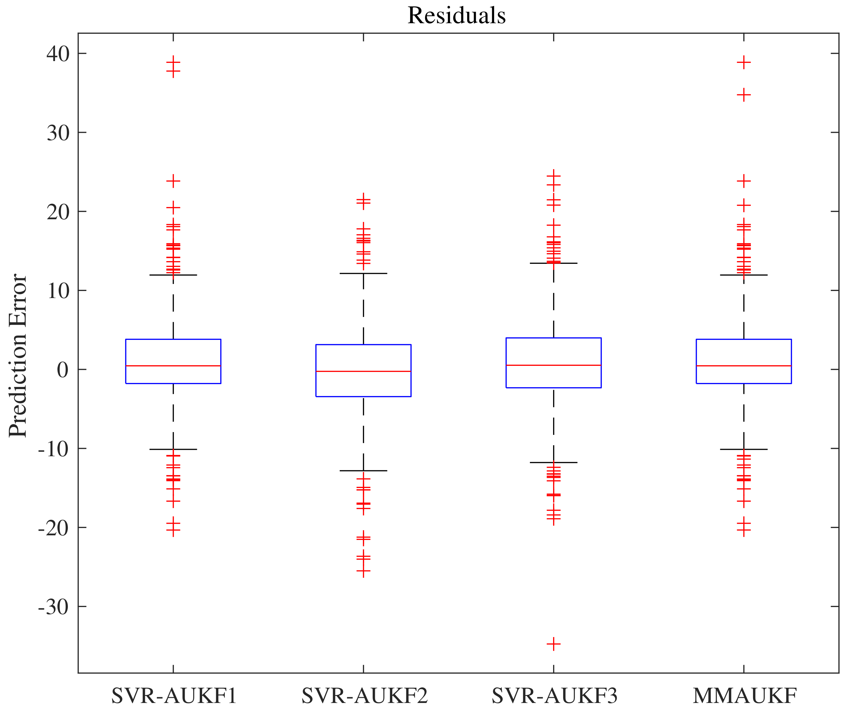
In Figure 13, the precision of MMAUKF is compared with the three single model of SVR-AUKF to predict PM 2.5 concentration. The MAE of MMAUKF method is 4.0492, the MAPE is 9.5337, the RMSE is 5.9130. The MAE of SVR-AUKF1 is 4.1994, the MAPE is 9.6523, and the RMSE is 6.2302. The MAE of SVR-AUKF2 is 4.3706, the MAPE is 10.7784, and the RMSE is 5.9424. The MAE of SVR-AUKF3 is 4.4815, the MAPE is 11.8585 and the RMSE is 6.2018. By the comparison of statistical errors, the error of MMAUKF method is smaller than the other method, and the proposed method overcomes that a single model cannot predict PM 2.5 concentration accurately under different time periods. The Table 2 shows the statistical errors based on SVR-AUKF methods for PM 2.5 concentration in three time periods. The boxplot of prediction residuals is shown in Figure 14,
Figure 14 shows that 75% of the residual error predicted by the proposed MMAUKF method is approximately up to 4, which is smaller than other methods. Thus, the proposed MMAUKF method is more accurate for predicting PM 2.5 concentration. The proposed MMAUKF method and SVR-AUKF, AR-Kalman, AR and BP methods is used to predicted PM 2.5 concentration in Figure 15.
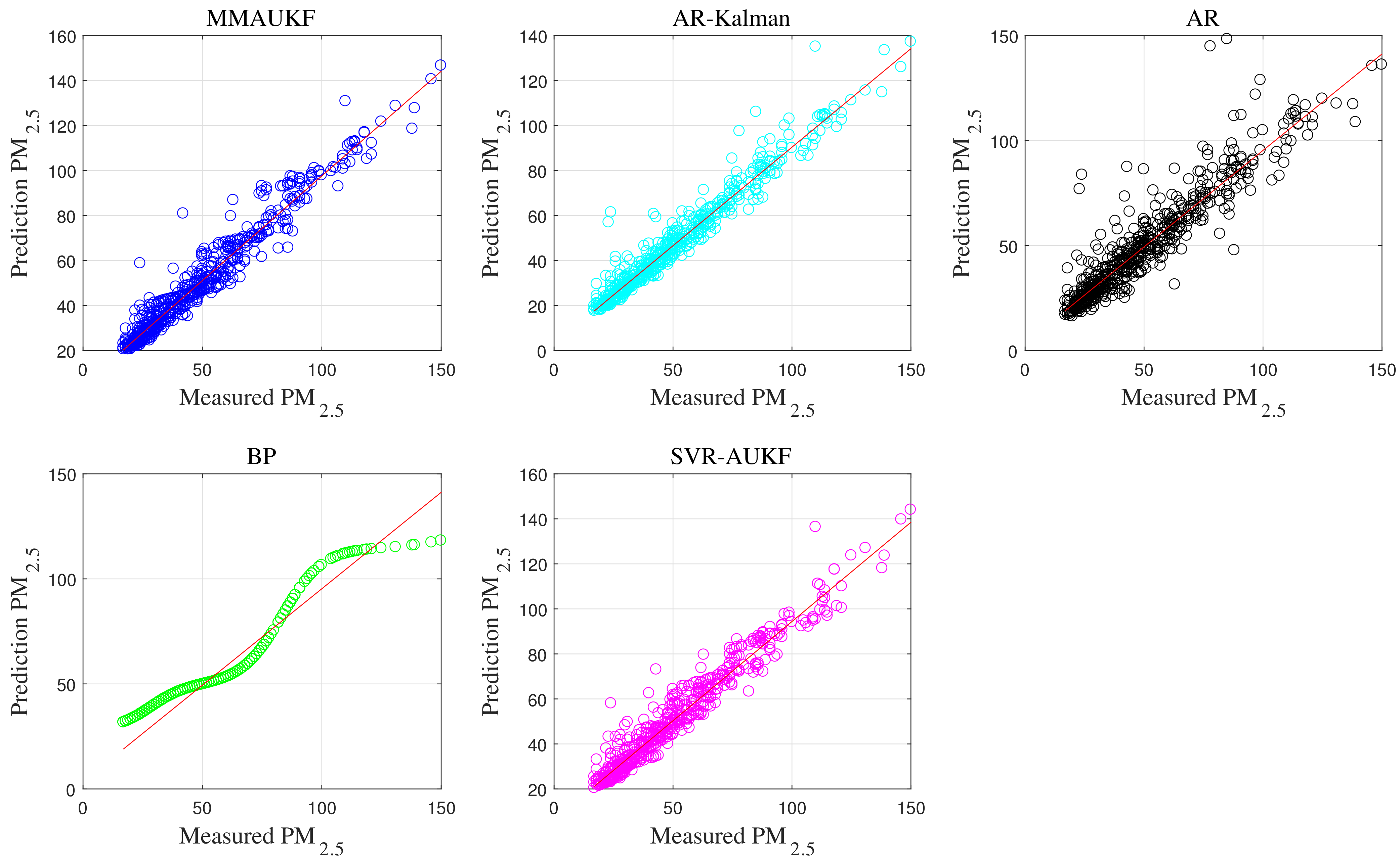
The prediction results of the proposed method is displayed, the fitting results between the predicted values and the actual values for different methods are shown in Figure 16.
It can be seen from Figure 16 that the fit result of MMAUKF method is better than the other prediction methods. Figure 15 shows the comparison between the proposed method and other methods. The statistical error is shown in Table 3. The MAE is 4.0492, the MAPE is 95,337 and the RMSE is 5.9130. The prediction accuracy of other methods is not as good as the proposed method. The proposed MMAUKF method provides better prediction results than other single model methods. The proposed MMAUKF method can globally predict the PM 2.5 concentration in the next hour, and which has good stability.
In order to better reflect the prediction accuracy of the proposed method, the prediction residuals for different methods are given by the method of statistical analysis. The prediction errors of proposed MMAUKF method and SVR-AUKF, ARKalman, AR and BP methods are shown Figure 17.
It can be seen from Figure 17 that the residual error of 75% of the proposed MMAUKF method is very small. The results show the prediction accuracy has been improved. In this section, the proposed MMAUKF method is used to predict PM 2.5 concentration, which has important practical significance to the public. The prediction results have reference significance for government departments to establish early warning system, which reduces the impact of public travel and avoids people exposed to high PM 2.5 concentration for a long time.

6. Conclusions

Previous studies found that PM 2.5 will affect people’s life and travel. In order to protect people from the impact of PM 2.5 concentration on air quality, an accurate PM 2.5 concentration prediction model that can deal with different environments is an urgent requirement. In this paper, the multiple model adaptive unscented Kalman filter (MMAUKF) is proposed to predict the atmospheric PM 2.5 concentration in the next hour. In addition, to evaluate the prediction applicability effect of the proposed method on PM 2.5 concentration in a campus in the previous hour. The proposed MMAUKF method is compared with SVR-AUKF, AR-Kalman, AR and BP methods. The error performance index of several different methods is analyzed, which includes MAE, MAPE and RMSE. The box chart of statistical analysis is given. The experimental results show that the proposed method has the smallest error and can accurately predict PM 2.5 concentration in different time periods. The MAE of the proposed MMAUKF method is 4.0492, MAPE is 9.5337 and RMSE is 5.9130. The prediction results fully show that the multiple model prediction method overcomes the shortcomings of the single model which is easily affected by the environment. The proposed method not only guarantees the accuracy of predicting PM 2.5 concentration when the noise is inaccurate, but also overcomes the limitations of the single model method. The validity and effectiveness of the proposed method is also proved. The PM 2.5 concentration is also closely related to spatial distribution. In the future, PM 2.5 concentration spatial dynamic model and tracing to the source may be considered and studied, which is combined with advanced prediction algorithm to predict PM 2.5 concentration more accurately.

Author Contributions

Conceptualization, J.L. and X.L.; methodology, J.L.; software, J.L.; validation, K.W., X.L. and J.L.; formal analysis, J.L.; investigation, J.L.; resources, X.L.; data curation, J.L.; writing—original draft preparation, J.L.; writing—review and editing, J.L.; visualization, K.W., G.C. and J.L.; supervision, X.L.; funding acquisition, X.L. All authors have read and agreed to the published version of the manuscript.

Funding

This study is support by Beijing Natural Science Foundation (4204087), National Key Research and Development Project (2018YFB1702704, 2018YFC1602704) and the National Natural Science Foundation of China (61873006, 61673053).

Data Availability Statement

The pollutant and meteorological data used in this study was obtained from the ongoing monitoring system of Beijing University of Technology. The monitoring system includes data from regional monitoring stations.

Acknowledgments

The author would like to thank other members of this paper for their contributions.

Conflicts of Interest

The authors declare no conflict of interest.

References

  1. Gao, J.; Tian, H.; Cheng, K.; Lu, L.; Zheng, M.; Wang, S.; Hao, J.; Wang, K.; Hua, S.; Zhu, C.; et al. The variation of chemical characteristics of PM2.5 and PM10 and formation causes during two haze pollution events in urban Beijing, China. Atmos. Environ. 2015, 107, 1–8. [Google Scholar] [CrossRef]
  2. Wang, Y.X.; Jiang, H.; Zhang, S.Q.; Xu, J.H.; Lu, X.H.; Jin, J.X.; Wang, C.L. Estimating and source analysis of surface PM2.5 concentration in the Beijing–Tianjin–Hebei region based on MODIS data and air trajectories. Int. J. Remote Sens. 2016, 37, 4799–4817. [Google Scholar] [CrossRef]
  3. Peng, W.; Ge, S.; Liu, Z.; Furuta, Y. Adsorption characteristics of sulfur powder by bamboo charcoal to restrain sulfur allergies. Saudi J. Biol. Sci. 2016, 24, 103–107. [Google Scholar] [CrossRef] [Green Version]
  4. You, S.; Tong, Y.W.; Neoh, K.G.; Dai, Y.; Wang, C.H. On the association between outdoor PM2.5 concentration and the seasonality of tuberculosis for Beijing and Hong Kong. Saudi J. Biol. Sci. 2016, 218, 1170–1179. [Google Scholar] [CrossRef] [PubMed] [Green Version]
  5. Wang, Y.; Kloog, I.; Coull, B.A.; Kosheleva, A.; Zanobetti, A.; Schwartz, J.D. Estimating Causal Effects of Long-Term PM2.5 Exposure on Mortality in New Jersey. Environ. Health Perspect. 2016, 124, 1182–1188. [Google Scholar] [CrossRef] [PubMed] [Green Version]
  6. Kavousi-Fard, A.; Samet, H.; Marzbani, F. A new hybrid modified firefly algorithm and support vector regression model for accurate short term load forecasting. Expert Syst. Appl. 2014, 41, 6047–6056. [Google Scholar] [CrossRef]
  7. Sun, W.; Sun, J. Daily PM2.5 concentration prediction based on principal component analysis and LSSVM optimized by cuckoo search algorithm. J. Environ. Manag. 2017, 188, 144–152. [Google Scholar] [CrossRef]
  8. Zhang, Y.; Lang, J.; Cheng, S.; Li, S.; Zhou, Y.; Chen, D.; Zhang, H.; Wang, H. Chemical composition and sources of PM1 and PM2.5 in Beijing in autumn. Sci. Total Environ. 2018, 630, 72–82. [Google Scholar] [CrossRef]
  9. Cobourn, W. An enhanced PM2.5 air quality forecast model based on nonlinear regression and back-trajectory concentrations. Atmos. Environ. 2010, 44, 3015–3023. [Google Scholar] [CrossRef]
  10. Elangasinghe, M.A.; Singhal, N.; Dirks, K.N.; Salmond, J.A.; Samarasinghe, S. Complex time series analysis of PM10 and PM2.5 for a coastal site using artificial neural network modelling and k-means clustering. Atmos. Environ. 2014, 94, 106–116. [Google Scholar] [CrossRef]
  11. Voukantsis, D.; Karatzas, K.; Kukkonen, J.; Räsänen, T.; Karppinen, A.; Kolehmainen, M. Intercomparison of air quality data using principal component analysis, and forecasting of PM10 and PM2.5 concentrations using artificial neural networks, in Thessaloniki and Helsinki. Sci. Total Environ. 2014, 140, 220–232. [Google Scholar] [CrossRef] [PubMed]
  12. Zhou, Q.; Jiang, H.; Wang, J.; Zhou, J. A hybrid model for PM2.5 forecasting based on ensemble empirical mode decomposition and a general regression neural network. Sci. Total Environ. 2014, 496, 264–274. [Google Scholar] [CrossRef]
  13. Zhan, Y.; Luo, Y.; Deng, X.; Chen, H.; Grieneisen, M.L.; Shen, X.; Zhu, L.; Zhang, M. Spatiotemporal prediction of continuous daily PM2.5 concentrations across China using a spatially explicit machine learning algorithm. Atmos. Environ. 2017, 155, 129–139. [Google Scholar] [CrossRef]
  14. Kadlyala, A.; Kumar, A. Vector—time—series—based back propagation neural network modeling of air quality inside a public transportation bus using available software. Environ. Prog. Sustain. Energy. 2017, 35, 7–13. [Google Scholar] [CrossRef]
  15. Das Chagas Moura, M.; Zio, E.; Lins, I.D.; Droguett, E. Failure and reliability prediction by support vector machines regression of time series data. Reliab. Eng. Syst. Saf. 2011, 96, 1527–1534. [Google Scholar] [CrossRef]
  16. Sivakumar, S. Marginally Stable Triangular Recurrent Neural Network Architecture for Time Series Prediction. IEEE Trans. Cybern. 2018, 48, 2836–2850. [Google Scholar] [CrossRef]
  17. Dai, X.L.; Liu, J.J.; Li, Y.L. A recurrent neural network using historical data to predict time series indoor PM2.5 concentrations for residential buildings. Indoor Air. 2021, 1–10. [Google Scholar] [CrossRef]
  18. Qiu, X.; Ren, Y.; Suganthan, P.N.; Amaratunga, G.A. Empirical Mode Decomposition based ensemble deep learning for load demand time series forecasting. Appl. Soft. Comput. 2017, 54, 246–255. [Google Scholar] [CrossRef]
  19. Cassola, F.; Burlando, M. Wind speed and wind energy forecast through Kalman filtering of Numerical Weather Prediction model output. Appl. Energy 2012, 99, 154–166. [Google Scholar] [CrossRef]
  20. Cassola, F.; Burlando, M. Short-term load forecasting using SVR (support vector regression)-based radial basis function neural network with dual extended Kalman filter. Energy 2013, 49, 413–422. [Google Scholar]
  21. Nasseri, M.; Moeini, A.; Tabesh, M. Forecasting monthly urban water demand using Extended Kalman Filter and Genetic Programming. Expert Syst. Appl. 2011, 38, 7387–7395. [Google Scholar] [CrossRef]
  22. Santamaría-Bonfil, G.; Reyes-Ballesteros, A.; Gershenson, C. Wind speed forecasting for wind farms: A method based on support vector regression. Renew. Energy 2016, 85, 790–809. [Google Scholar] [CrossRef]
  23. Bisoi, R.; Dash, P.K. A hybrid evolutionary dynamic neural network for stock market trend analysis and prediction using unscented Kalman filter. Appl. Softw. Comput. 2014, 19, 41–56. [Google Scholar] [CrossRef]
  24. Meng, J.; Luo, G.; Gao, F. Lithium Polymer Battery State-of-Charge Estimation Based on Adaptive Unscented Kalman Filter and Support Vector Machine. IEEE Trans. Power Electron. 2016, 31, 2226–2238. [Google Scholar] [CrossRef]
  25. Sun, F.; Hu, X.; Zou, Y.; Li, S.G. Adaptive unscented Kalman filtering for state of charge estimation of a lithium-ion battery for electric vehicles. Energy 2011, 36, 3531–3540. [Google Scholar] [CrossRef]
  26. Blom, H.A.P.; Bar-Shalom, Y. The interacting multiple model algorithm for systems with Markovian switching coefficients. IEEE Trans. Autom. Control. 1988, 33, 780–783. [Google Scholar] [CrossRef]
  27. Mazinan, A.H.; Sadati, N. Fuzzy predictive control based multiple models strategy for a tubular heat exchanger system. Appl. Intell. 2010, 33, 247–263. [Google Scholar] [CrossRef]
  28. Xie, G.; Gao, H.; Qian, L.; Huang, B.; Li, K.; Wang, J. Vehicle Trajectory Prediction by Integrating Physics- and Maneuver-Based Approaches Using Interactive Multiple Models. IEEE Trans. Ind. Electron. 2018, 33, 5999–6008. [Google Scholar] [CrossRef]
  29. Li, X.L.; Jia, C.; Wang, K.; Wang, J. Trajectory tracking of nonlinear system using multiple series-parallel dynamic neural networks. Neurocomputing 2015, 168, 1–12. [Google Scholar] [CrossRef]
  30. Li, X.L.; Jia, C.; Liu, D.X.; Ding, D.W. Nonlinear adaptive control using multiple models and dynamic neural networks. Neurocomputing 2014, 136, 190–200. [Google Scholar] [CrossRef]
  31. Li, X.L.; Zhang, X.F.; Jia, C.; Liu, D.X. Multi-model adaptive control based on fuzzy neural networks. J. Intell. Fuzzy Syst. 2014, 27, 965–975. [Google Scholar] [CrossRef]
  32. Li, X.L.; Liu, D.X.; Jia, C.; Chen, X.Z. Multi-model control of blast furnace burden surface based on fuzzy SVM. Neurocomputing 2014, 148, 209–215. [Google Scholar] [CrossRef]
  33. Breeton, R.G.; Lloyd, R.G. Support Vector Machines for classification and regression. Analyst 2009, 23, 230–267. [Google Scholar]
  34. Yang, W.; Deng, M.; Xu, F.; Wang, H. Prediction of hourly PM2.5 using a space-time support vector regression model. Atmos. Environ. 2018, 181, 12–19. [Google Scholar] [CrossRef]
  35. Li, X.L.; Luo, A.R.; Li, J.G.; Li, Y. Air Pollutant Concentration Forecast Based on Support Vector Regression and Quantum-Behaved Particle Swarm Optimization. Atmos. Environ. 2019, 24, 205–222. [Google Scholar] [CrossRef]
  36. Smola, A.; Scholköpf, B. A tutorial on support vector regression. Stat. Comput. 2004, 14, 199–222. [Google Scholar] [CrossRef] [Green Version]
  37. Gass, S.I.; Fu, M.C. Karush-Kuhn-Tucker (KKT) Conditions. In Encyclopedia of Operations Research and Management Science; Springer: New York, NY, USA, 2013; pp. 833–834. [Google Scholar]
  38. Chen, K.; Yu, J. Short-term wind speed prediction using an unscented Kalman filter based state-space support vector regression approach. Appl. Energy 2014, 113, 690–705. [Google Scholar] [CrossRef]
  39. Liu, H.; Tian, H.; Li, Y. Comparison of two new ARIMA-ANN and ARIMA-Kalman hybrid methods for wind speed prediction. Appl. Energy 2012, 98, 415–424. [Google Scholar] [CrossRef]
  40. Wang, Z.; Chen, L.; Ding, Z.; Chen, H. An enhanced interval PM2.5 concentration forecasting model based on BEMD and MLP~1 with influencing factors. Atmos. Environ. 2020, 223, 117200.1–117200.16. [Google Scholar] [CrossRef]
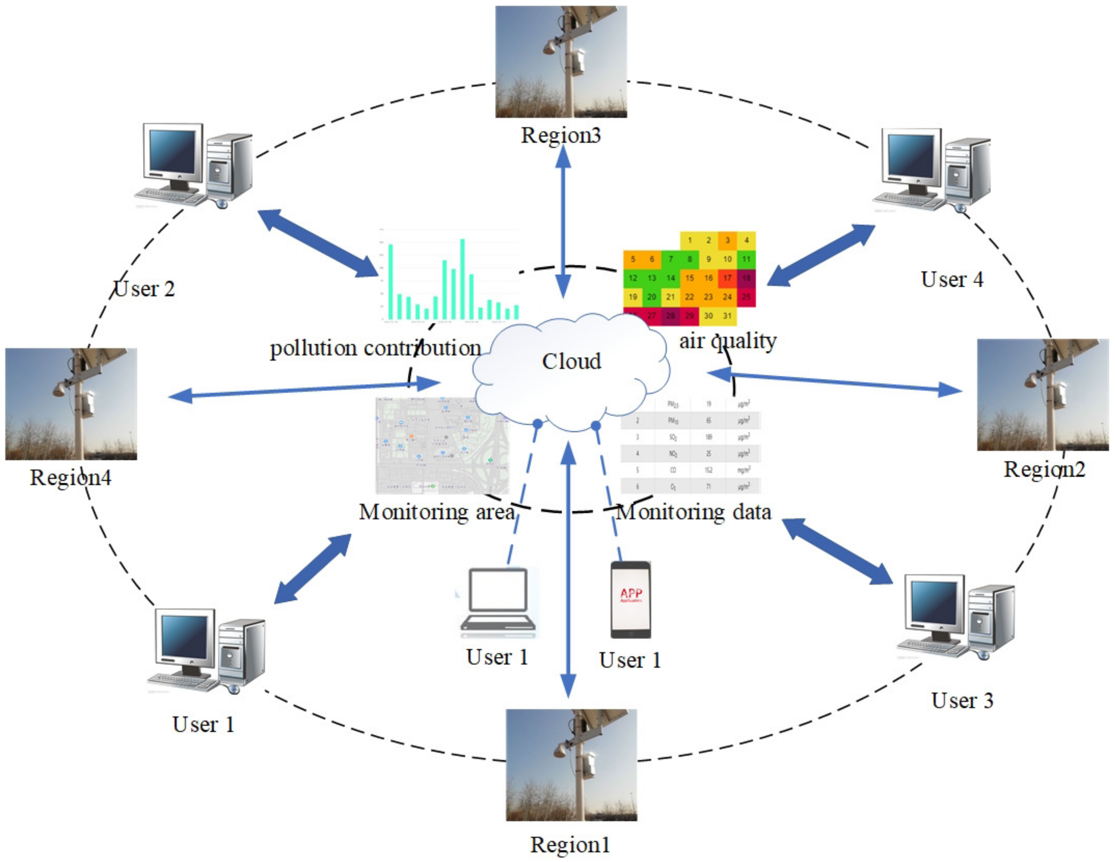
Figure 1. Schematic of atmospheric data monitoring platform.
Atmosphere 12 00607 g001
Figure 2. The scatterplot of PM 2.5 concentration with other monitored variables.
Atmosphere 12 00607 g002
Figure 3. The schematic diagram of the SVR-AUKF algorithm for PM 2.5 concentration prediction.
Atmosphere 12 00607 g003
Figure 4. The PM 2.5 concentration prediction of single SVR-AUKF method.
Atmosphere 12 00607 g004
Figure 5. The modeling data of PM 2.5 concentration in three time periods.
Atmosphere 12 00607 g005
Figure 6. The structure chart of the MMAUKF method for PM 2.5 concentration prediction.
Atmosphere 12 00607 g006
Figure 7. The PM 2.5 concentration prediction of SVR-AUKF1.
Atmosphere 12 00607 g007
Figure 8. Boxplot of SVR-AUKF1 prediction residuals.
Atmosphere 12 00607 g008
Figure 9. The PM 2.5 concentration prediction of SVR-AUKF2.
Atmosphere 12 00607 g009
Figure 10. Boxplot of SVR-AUKF2 prediction residuals.
Atmosphere 12 00607 g010
Figure 11. The PM 2.5 concentration prediction of SVR-AUKF3.
Atmosphere 12 00607 g011
Figure 12. Boxplot of SVR-AUKF3 prediction residuals.
Atmosphere 12 00607 g012
Figure 13. The comparison results of the proposed MMAUKF method and three single SVR-AUKF methods.
Atmosphere 12 00607 g013
Figure 14. Boxplot of SVR-AUKF1, SVR-AUKF2, SVR-AUKF3 and MMAUKF prediction residual.
Atmosphere 12 00607 g014
Figure 15. The comparison results of the proposed MMAUKF method and SVR-AUKF, AR-Kalman, AR and BP methods.
Atmosphere 12 00607 g015
Figure 16. Boxplot of different methods’ prediction residual.
Atmosphere 12 00607 g016
Figure 17. The comparison results of the proposed MMAUKF method and SVR-AUKF, AR-Kalman, AR and BP methods.
Atmosphere 12 00607 g017
Table 1. Descriptive statistics of pollutants and meteorological conditions.
UnitMeanStandard Deviation
PM 2.5 µg/m351.3724.38
PM 10 µg/m371.2029.99
SO 2 µg/kg5.574.38
NO 2 mg/m328.7711.84
COmmol/L0.980.41
O 3 mg/m127.0465.70
RH%31.504.28
T ° C71.2119.42
Table 2. The error performance index of three SVR-AUKF and MMAUKF methods.
MethodMAEMAPE(%)RMSE
MMAUKF4.04929.53375.9130
SVR-AUKF14.19949.65236.2302
SVR-AUKF24.370610.77845.9424
SVR-AUKF34.481511.85856.2018
Table 3. The error performance index of MMAUKF and other single model methods.
MethodMAEMAPE(%)RMSE
MMAUKF4.04929.53375.9130
SVR-AUKF4.23049.77046.1347
AR-Kalman5.0710.26216.8705
AR5.873512.77059.5259
BP7.217321.29408.3226
Publisher’s Note: MDPI stays neutral with regard to jurisdictional claims in published maps and institutional affiliations.