Article

Evaluating the NDVI–Rainfall Relationship in Bisha Watershed, Saudi Arabia Using Non-Stationary Modeling Technique

1
Department of Civil Engineering, College of Engineering, King Khalid University, Abha 61411, Saudi Arabia
2
Department of Chemical Engineering, College of Engineering, King Khalid University, Abha 61411, Saudi Arabia
3
Department of Biological and Agricultural Engineering, Texas A & M University, College Station, TX 77843-2117, USA
4
Department of Energy and Environment, TERI School of Advanced Studies, New Delhi 110070, India
*
Author to whom correspondence should be addressed.
Atmosphere 2021, 12(5), 593; https://doi.org/10.3390/atmos12050593
Submission received: 16 March 2021 / Revised: 25 April 2021 / Accepted: 29 April 2021 / Published: 2 May 2021
(This article belongs to the Section Biosphere/Hydrosphere/Land–Atmosphere Interactions)

Abstract

:
The Normalized Difference Vegetation Index (NDVI) and rainfall data were used to model the spatial relationship between vegetation and rainfall. Their correlation in previous studies was typically based on a global regression model, which assumed that the correlation was constant across space. The NDVI–rainfall association, on the other hand, is spatially non-stationary, non-linear, scale-dependent, and influenced by local factors (e.g., soil background). In this study, two statistical methods are used in the modeling, i.e., traditional ordinary least squares (OLS) regression and geographically weighted regression (GWR), to evaluate the NDVI–rainfall relationship. The GWR was implemented annually in the growing seasons of 2000 and 2016, using climate data (Normalized Vegetation Difference Index and rainfall). The NDVI–rainfall relationship in the studied Bisha watershed (an eco-sensitive zone with a complex landscape) was found to have a stable operating scale of around 12 km. The findings support the hypothesis that the OLS model’s average impression could not accurately represent local conditions. By addressing spatial non-stationarity, the GWR approach greatly improves the model’s accuracy and predictive ability. In analyzing the relationship between NDVI patterns and rainfall, our research has shown that GWR outperforms a global OLS model. This superiority stems primarily from the consideration of the relationship’s spatial variance across the study area. Global regression techniques such as OLS can overlook local details, implying that a large portion of the variance in NDVI is unexplained. It appears that rainfall is the most significant factor in deciding the distribution of vegetation in these regions. Furthermore, rainfall had weak relationships with areas predominantly located around wetlands, suggesting the need for additional factors to describe NDVI variations. The GWR method performed better in terms of accuracy, predictive power, and reduced residual autocorrelation. Thus, GWR is recommended as an explanatory and exploratory technique when relations between variables are subject to spatial variability. Since the GWR is a local form of spatial analysis that aligned to local conditions, it has the potential for more accurate prediction; however, a larger amount of data is needed to allow a reliable local fitting.

1. Introduction

Satellite imagery is commonly used to assess the distribution and productivity of vegetation at large spatial scales. The most widely used multi-spectral vegetation index is the Normalized Difference Vegetation Index (NDVI). It exhibits a good correlation with green-leaf density and can be used to estimate above-ground biomass [1]. Remote sensing-derived NDVI data have been used to evaluate regional and global climatic and environmental changes. The NDVI has been used in various agricultural applications, including drought monitoring [1,2], prediction of crop yield [3,4], calculate crop phenological information [5], estimate the aboveground biomass [6], and land cover change detection [7,8]. It also used to monitor and investigate droughts [9,10,11] as well as expose the effects of global climate change [12,13], land degradation, and desertification [12,13,14,15,16,17,18]. Over the last 30 years, NDVI time series data has been widely used to assess changes in vegetation conditions and their relationship to climate change [19,20]. As a result, understanding and modeling the quantitative relationship between NDVI and climate is critical for NDVI applications in these fields.
Rainfall measurements based on remote sensing (onboard satellites) can provide sufficient data with high spatio-temporal resolution over extensive areas where traditional rain gauge data are scarce [21,22]. Though it has many disadvantages, the most important of which is significant ambiguity, since no satellite sensors observe or detect rainfall on their own, and the relationship between observations and it is dependent on one or more indirect variables [23,24]. There are currently a number of satellite observation data products related to rainfall obtained from different data sources such as “Climate Hazards Group InfraRed Rainfall with Stations (CHIRPS)”.
From 1981 to the present, the CHIRPS product offers daily precipitation data with a spatial resolution of 0.05° for the quasi-global coverage of 50° N–50° S. The “USGS-Earth Resources Observation and Science (EROS)” center developed the product with the collaboration of the “Santa Barbara Climate Hazards Unit, University of California” [22]. Information related to the CHIRPS procedure and production could be found in Tote et al. [24]. Rainfall measurements calibrated using remote sensing (on-satellite) versus rain gauge data could increase the precision of estimated rainfall data [25]. Several validation studies were carried out in Colombia [22,26], Southwestern North America [22], Southeastern Africa [24], the Sahel in Africa [27,28], Brazil [29], Asir Province, Saudi Arabia [30], and Mainland China [31]. Limitations of CHIRPS data [31] are as follows, the CHIRPS rainfall model is primarily based on an IR-based statistical model. The CHIRPS performs well in tropical areas but not in middle latitudes. Compared to arid and semi-arid land, CHIRPS performs better in areas where there is a considerable amount of rainfall. Furthermore, changes in good performance zones are strongly linked to monsoon movement. In general, CHIRPS accuracy is higher in the summer than in the winter. Its ability to detect snowfall of any severity is minimal. The rainfall from typhoon weather systems is moderately vulnerable to CHIRPS.
Several earlier studies modeled relationships between NDVI trends and climatic factors on a spatial or temporal scale. The most common empirical metrics used to determine the relationships in most of these studies were statistical regression and correlation techniques. In arid areas, NDVI and rainfall have strong correlations [32,33,34]. For each region and landscape, the relationship between NDVI and eco-climatic predictors is different. The known causes of variability in relationships between NDVI and its independent variable are spatial variations in soil conditions or vegetation type [32,35,36]. NDVI varies due to local climatic conditions, such as temperature and rainfall, and this correlation is widely known across varying spatio-temporal scales [37,38,39,40]. Precipitation appears to be a key predictor of vegetation distribution, particularly in environments transitioning from humid to arid or semi-arid conditions [37,41,42]. NDVI is often modeled as a variable of rainfall in most studies that explain the relationship between vegetation and rainfall, using global linear models calibrated such as “Ordinary Least Squares” (OLS) regression methods [43].
When modeling the spatial relationship between NDVI and climate, it is necessary to consider the relationship’s non-stationarity in space. However, in a spatial context, the traditional statistical regression approach (OLS) is stationary. Stationarity refers to fitting a single model to all data and its application uniformly over the whole geographical area of interest. This regression model and its coefficients are spatially constant, meaning the relationship is spatially constant as well. This seems to be often insufficient when dealing with spatially differentiated data, particularly while evaluating relationships at global or regional scales. The magnitude and sign of model parameters can differ significantly between regression models created in different locations. Developing an independent OLS model for each land use/cover or vegetation type is the simplest way to refine the regression model and reduce these variations. The variance in regression parameters between land cover classes can be illustrated in this way, and the regression model’s predictive power improves significantly [32,35,36]. However, the local non-stationarity in the relationship within the land cover form is not considered by this approach.
Allowing the model’s parameters to vary with space is an interesting and effective alternative. Since the model fitted locally is more aligned to local conditions, such non-stationary modeling has the potential for more accurate prediction. Local regression techniques such as localized OLS (moving window regression) or geographically weighted regression (GWR) can help solve the non-stationarity problem and quantify regression model parameters that vary spatially. Recently, it has been recognized that the GWR [44,45,46], as a local regression model, is capable of exploring spatially varying correlation through an application in the fields of human geography [47,48] and ecology [49,50]. GWR facilitates the relationships between dependent and explanatory variables to change over time, effectively dealing with residual correlation and non-stationarity. The outcomes of this local method may be useful for explanatory purposes, such as detecting areas of model measurement errors or areas with remarkable variations that would else be missed in a global model [30]. In large spatial scale landscape ecology, standard statistical tests such as the “Akaike Information Criterion (AIC) or cross-validation scores (CV)” indicate that the GWR model is better implemented than OLS models [37]. There are only a few studies in the field of remote sensing that employ local regression techniques to analyze spatial relationships between satellite imagery and climatic variables [51,52,53].
The present study examines spatial relationships between NDVI data from the MODIS NDVI satellite data and rainfall data from CHIRPS in the Bisha Watershed in south-western Saudi Arabia. This study area is considered sensitive to environmental changes because it exists as an eco-climatic transition zone between cold semi-arid and hot arid climates (extended from south to north) [30,54,55]. According to the “Köppen climate classification [56,57]” transition areas, which are usually semi-arid and change from sub-humid climates to desert climates, have semi-arid climates, as well as certain ecological characteristics that transition between them. Many scientists are concentrating on the North China transition zone to investigate such relationships between NDVI and climatic factors [58,59]. Fewer studies, however, have looked into the various effects of climatic variables like temperature, rainfall, and humidity, as well as scale dependence and spatial stationary on vegetation in this area. Given the high spatial variability of climate conditions, it is worthwhile to investigate the variations in climate effects on vegetation between transition zones and surrounding areas. As a result, investigating these issues with GWR as a tool to investigate these issues and potentially improve modeling of the NDVI–rainfall relationship in the area would be very important.
Indeed, the majority of the issues raised in this study are well-known to geostatistics experts and have been investigated in geostatistical methods for many years. Local regression models, however, have yet to achieve general acceptance in the international literature on ecology and environmental science. As a result, the authors of these papers did not set out to innovate in the area of geostatistical data analysis techniques. Rather than that, this study should be viewed as a contribution to the ongoing debate in ecology and environmental science about local and global approaches to spatial data analysis.
Thus, the study’s objective is to use non-stationary modeling techniques to investigate the spatial variation in the NDVI–rainfall relationship in the Bisha Watershed between the growing seasons of 2000 and 2016. The total amount of rainfall in the region varied significantly in these two years, with 2000 being a relatively dry year and 2016 being a rainy year. The use of several growing seasons enables the investigation of temporal variations in spatial relationships. An attempt was made to classify areas most vulnerable to seasonal rainfall variability by analyzing the surrounding local regression results. This study aims to address the following issue investigations into areas vulnerable to spatio-temporal dynamics. These findings may be useful to ecologists studying climate change and vegetation distribution in the area.

2. Materials and Methods

2.1. Study Area

The study is in the Bisha watershed, situated in the south-western part of Saudi Arabia. The area is 21,260 km2 in size and touches a few distance borders with Yemen. The Bisha watershed boundary found in between the latitude of 17°59′27.588″ N and 20°49′13.958″ N and longitude of 41°49′50.825″ E and 43°11′20.254″ E. It has varied geography that includes highlands, high mountains (2000 to 3000 m above sea level), plateau, and Wadiyan. It also encompasses a wide portion of the desert to the north and east, all the way to the cities of Bisha and Tathlith. The topography ranges from 950 to 2980 m with a mean of 1655 m and std. dev. of 403.44 (Figure 1). Geologically, it comprises of sedimentary rocks, (limestone, sandstone, shale) of Jurassic-Cretaceous and Precambrian granite igneous rocks basement [54]. The climate of the region varies greatly depending on geography and season.
The study area’s climate ranges from semi-arid to arid, depending on the direction one travels south to north. The study region is served by three meteorological stations run by Saudi Arabia’s Presidency of Meteorology and Environment (PME). Meteorological station locations are illustrated in Figure 1. According to data from three stations over the last 30 years, the average temperature ranges between 12° C and 44° C. Figure 2 depicts temperature statistics for the years 2000 and 2016 from three meteorological stations: (a) Abha; (b) Khamis Mushyet; and (c) Bisha (March–June). Due to a lack of a sufficient number of meteorological stations in the study area, the spatial variation of temperature input analysis is not performed. The data from the three stations, on the other hand, indicate that temperature variation was very significantly low in 2000 and 2016.
The south–west monsoon brings variable rainfall to the highlands of this region [54,60]. In the studied watershed, the high rainfall occurs during the spring and summer is spread out over 2–4 months (March–June), whereas rainfall for the remainder of the period is insignificant [61]. The watershed’s rugged landscape has helped in the conservation of the region’s biodiversity. This watershed is also home to one of the extinct natural habitats for the Arabian leopard, listed in The International Union for Conservation of Nature (IUCN) Red List as critically endangered [62]. There is also a corresponding phytogeographic area known as the Afromontane, which is part of the studied watershed [63]. The highland of the watershed is surrounded by numerous forests and Juniperus procera, where many endemic and rare plants and animals live [64].

2.2. Normalized Difference Vegetation Index (NDVI)

Descriptions of datasets from multiple sources used in the current study are given as (a) MODIS NDVI: spatial resolution of 250 m, 16-day composite grid data L3 product (MOD13Q1) was obtained from NASA Earth Observation System (EOS) data gateway for March–April–May–June 2000 and March–April–May–June 2016. MODIS NDVI data have been rectified onto UTM WGS84 and resampled to a 250 m, subsequently layer stacking and region of interest (ROI) subsetting. The NDVI value given in MOD13Q1 products is an integer (16 bits) and ranges between −2000 and 10,000. To convert these values in NDVI, “true” values were necessary to apply a scale factor. Therefore, all the original data were multiplied by 0.0001. Daily images were consisted semi-monthly using the maximum recorded value NDVI to ensure that any residual cloud coverage would have the minimal effect on our results [65]. NDVI was integrated (NDVImax) over the growing season (March–June) for each year (2000 and 2016) to have a yearly estimate of vegetation productivity during the growing season.

2.3. Climate Hazard InfraRed Precipitation with Stations (CHIRPS)

The “CHIRPS v.2.0” has a rainfall dataset that is available at a 3 km grid. Gridded precipitation datasets are created from rain gauge observations, and geostationary infrared satellite rainfall estimates interpolated to create these data [22]. Monthly grids were downloaded for the period of 2000 and 2016 (March to June) (ftp://ftp.chg.ucsb.edu/pub/org/chg/products/CHIRPS-2.0) (access on 30 April 2021). The periods have been chosen due to the substantial variance in cumulative rainfall (March to June) from 2000 to 2016. “The descriptive statistics of cumulative rainfall data from March to June during the rainy season are shown in Table 1.
Nearest neighbor interpolation was used to reproject and resample all CHIRPS datasets to match with the NDVI dataset. While there are various resampling techniques available, we chose this method to maintain the original dataset values [66] and avoid the resampling variations reported in the literature [67].

2.4. Methods of Modeling

The spatial analysis used “Ordinary Least Squares (OLS) and geographically weighted regression (GWR) models” to compare NDVI and rainfall data. The coefficients obtained from the regression equations for the NDVI–rainfall relationship to quantify the rainfall gradients in the Bisha watershed.

2.4.1. Ordinary Least Squares (OLS) Model

In a linear regression model, the OLS technique is used to estimate the unknown variables. Equation (1) shows the linear model of the OLS method
y i = β 0 + β i ( x i ) + ε
where y i = dependent variable (NDVI), β 0 = intercept, β 1 = estimated coefficient, x i = independent variable (rainfall), ε = error, and p = no. of independent variables. The OLS regression method’s stationary characteristics indicate that a unilateral model is employed to the whole watershed and is distributed homogeneously across the watershed area. In the OLS regression model, the relationship is assumed to be constant geographically, and the coefficients are assumed to be constant as well. It does not refer to a predefined, same linear relationship between diverse arid and semi-arid and mountainous watershed settings.

2.4.2. Geographically Weighted Regression Model (GWR)

The GWR model was designed to extend the traditional global regression method that works with empirical relationships that are spatially non-stationary. One of the best ways to treat spatial data is with a local regression method, which can be used to find optimal solutions for certain data that have some degree of spatial dependence [68]. The method distributes locally linked information and enables regression model variables to differ spatially. GWR aims to verify the spatial phenomenon of non-stationarity as a relationship between a number of a dependent variable and independent variables. Fotheringham et al. [69] provide a detailed theoretical background and overview of the algorithm. The GWR principle allows local variables to be derived as local rather than global variables [56], which account for spatially dependent correlation between NDVI and rainfall (Equation (2)).
y i = β 0 ( u i , v i ) + β 1 ( u i , v i ) x i + ε i
where y i and x i are NDVI and rainfall at the location ( u i , v i ) , ε i is the residual at the ( u i , v i ) , that is assumed to be distributed randomly, in addition, β 0 and β 1 are the regression coefficients (viz. intercept and slope) at the location ( u i , v i ) , two coefficients are calculated by least-weighted approach (Equation (3)). The neighbor location weight (j) on location ( u i , v i ) uses the function of Equation (4). The weight calculation is based on the distances ( d i j ) between the location (ui, vi) and the neighbor location (ui, vi). In particular, locations closer to the origin have a higher weight on the coefficient estimation at location (ui, vi). In coefficient estimation, the bandwidth ( h ) defining the radius to include neighboring locations is optimized by cross-validation Equation (5). Optimal bandwidth is derived by minimizing the sum of squared errors during cross-validation. Specifically, the error term in Equation (5) refers to the difference between estimated NDVI ( y ^ ( h ) ) and observed NDVI ( y i ) for each point (i) used in the cross-validation and both OLS and GWR models were executed by using the spatial-statistical extensions in ArcGIS.”
β ^ ( u i , v i ) = [ Χ T W ( u i , v i ) X ] 1 X T W ( u i , v i ) Y
w j ( u i , v i ) = exp [ ( d i j h ) 2 ]
C V S S = i = 1 n [ y i y ^ ( h ) ] 2

2.4.3. Model Performance Evaluation

The R2 coefficient is used to measure the goodness of fit of GWR and OLS models [70]. The higher the goodness of fit for the observations, the greater the coefficient. The R2 value is between 0% (0) and 100% (1.0), indicating the strength of the linear relationship between x and y. The higher R2 value suggests a better understanding of the variables that are responsible for the variance in the dependent variable. In addition to that, R2-based interpretation of the statistical result may be biased. If a small bandwidth is chosen, the R2 value will be high. The value of the Akaike Information Criterion (AIC) was therefore integrated with R2 to verify the efficiency of the model. To test the prediction accuracy of OLS and GWR, two output indices such as Root Mean Square Error (RMSE) and Mean Absolute Error (MAE) were employed.
R M S E = i = 1 N [ z i * z i ] 2 N
M A E = 1 N i = 1 N [ z i * z i ]
where z i * = predicted value and z i = observed value.

2.4.4. Measuring Spatial Autocorrelations

The geostatistical model characteristics based on projected data and observed are evaluated using spatial autocorrelation analysis. In this respect, important literature relating to the procedures for autocorrelation analysis is available [37]. To investigate the spatial autocorrelation of the NDVI data, the “global autocorrelation and local autocorrelation of the Moran’s I statistics” carried out in the current study. The mean of the spatial difference between all the spatial cells and their neighboring cells can be used to define the spatial characteristic of a given property in the whole study region using global spatial autocorrelation analysis [71]. The normalized z-score value varies from −1 to 1 in the Moran statistics. A Moran value greater than 0 indicates that there is a positive correlation with a cluster pattern, while a Moran value less than zero indicates that there is a negative correlation with a scattered pattern. The Moran’s I statistics for spatial autocorrelation were determined as shown in Equation (8) [72].
I = N i = 1 n j = 1 n w ij ( x i x ¯ ) ( x j x ¯ ) ( i = 1 n j = 1 n w ij ) i = 1 n ( x i x ¯ ) 2
where N = number of observations, Xi = observed value of cell i, Xj= observed the value of cell j, x ¯ = mean value of Xi, and Wij is the weighting value between the cell i and j [30]. The global spatial autocorrelation, the Moran I statistics only display the overall pattern of clustering, but it cannot be tested in several locations to detect spatial association patterns. Local Spatial Autocorrelation determines the importance of local statistics at each location and the location of spatial clusters, while global spatial autocorrelation does not. Local spatial autocorrelation, therefore, Moran’s I is being used to measure the local spatial relation and disparity between each grid location and its surrounding grid location [71]. Moran’s I local spatial autocorrelation is determined using Equation (9) [73].
I i = x i i = 1 , j i N w i j x j
where N = number of observations, Xi = observed value of cell i, Xj = observed the value of cell j, and Wij = weighting value between the cell i and j [30]. One of the methods to estimate the outcome of local spatial autocorrelation Moran’s I is by using z-score. The ArcGIS software was used to measure Moran’s I statistics in the current study. Local Moran’s I can be measured using z-score, just like the global OLS Moran’s I.

2.4.5. Scale Dependency of Non-stationarity

The stationarity Index (SI) introduced by Osborne et al. [74] is being used in environmental landscape to investigate the scale dependency of non-stationarity between environmental factors in obtaining reliable GWR results and choose a suitable bandwidth size. The SI is calculated using following equation:
S I = i q r g w r S E × 2
where, SI = stationarity index, iqrgwr = interquartile range of GWR coefficients, and SE = standard error of a global model coefficient [37].

3. Results

3.1. Rainfall Data Analysis

In Saudi Arabia, the watershed under investigation receives the most annual rainfall, spread out over four months (March to June). Figure 1 displays the average rainfall distribution of the rainy months (March–June) for 2000 and 2016. In 2000, the distribution of low rainfall years accounted for 73.4 mm on average, while the distribution of high rainfall in 2016 accounted 147.7 mm on average. The skewness (SK) of these two years (SK = 0.44 and 0.57 for 2000 and 2016, respectively) is nearly nil. In both years, there is a significant bias to the right, with a leptokurtic distribution. The kurtosis of the year of 2016 is 0.48, that proposes platykurtic distribution, whereas 2000 dataset illustrates the −0.65, proposing leptokurtic distribution.

3.2. Scale-Dependency Bandwidth

During the growing season, the correlation between NDVI–rainfall in the Bisha watershed was scale-dependent. As the bandwidth expanded and included data from distant locations, the regression coefficients smoothed out and became more similar to those of a global regression model. By comparison, narrow bandwidths allowed very detailed patterns while increasing higher standard errors.
The SI for both 2000 and 2016 (Figure 3) shows that non-stationary scale-dependence was observable by varying the investigation scale. The SI was greater for narrow bandwidth both years, whereas the SI index was firmed with the bandwidth broadened (stabilized). In any of the spatial scales examined, the index values were also not stationary, indicating high non-stationary data. The SI drops suddenly as bandwidth increases, stabilizing about 12 km, indicating that this is the appropriate scale for the NDVI–rainfall relationship, such as the minimum geographical area within which a consistent relationship for the entire region can be formed”This could be described as the size of a geographic landscape unit that determines the natural arrangement of the geographic phenomenon in which non-stationary variations could be implemented, thus eliminating unwanted noise and bias in the model.

3.3. The GWR and OLS Model Assessment

For 2000 and 2016 outputs, model comparisons were made between the GWR and OLS models. For both years, GWR had a much higher coefficient of determination (R2) than the OLS model (see Section 3.5). Section 3.5 contains a more detailed analysis. OLS models allow uneven estimations while GWR models deviate less. In both years, the F-test based on an ANOVA indicated that GWR provided statistically significant improvements over OLS models (p < 0.01). GWR statistics described more of variance and lowered AIC values (Yr. 2016 = −195,048; Yr. 2000 = −45,966) than OLS models (Yr. 2016 = −1,039,123; Yr. 2000 = −1,204,340), this describes the degree of freedom as well as model complexity changes.

3.4. The NDVI–Rainfall Relationship’s Spatial Pattern

The Normalized Difference Vegetation Index (NDVI) is a remote-sensing (satellite) derived vegetation index. The distinct colors (wavelengths) of visible and near-infrared sunlight reflected by plants are observed to determine the density of green on a patch of land [74]. NDVI has increasingly been used to assess various ecosystem resources, accounting for climate, land use, landscape, and soils, and a deviation from the norm implies either land loss or change. The NDVI–rainfall correlation has spatio-temporal variability in the Bisha watershed. To consider the geospatial variability of efficient bandwidth and related factors, GWR models provided maps of the standardized residuals (StdResid), slopes of the local regressions coefficients (β coefficients), and local R2.
Slope coefficients (beta coefficients) provide information about the magnitude and the type of relationship between variables. Since the vast majority of the coefficients are positive, it can be concluded that increased rainfall leads to an increase in NDVI. There is a broad variation in the rate of increase within the Bisha watershed (Figure 4). Relationships were stronger in the growing season of 2016 compared to 2000. Despite this, some very significant differences are identified in the maps. It should be noted that though the rainfall coefficient was lower in most of the part of Bisha watershed in 2016 than during the drier year of 2000, a seemingly large cluster that covers and extends over Bisha watershed suddenly has high rainfall coefficient values surpassing even all the coefficients for 2000 (Figure 4 and Figure 5). The results of this study indicate that NDVI is especially sensitive to changes in rainfall in that year. In a global model, these remarkable local variations would be lost. Apart from establishing a spatially continuous sensitive geographic transitional region, the Bisha watershed produces clusters (Figure 6) that act as transition zones, their size is dictated by the amount of rain they get, and they serve as intermediate corridors between humid semi-arid and hyper-arid environments. The cluster analysis in Figure 6 and Figure 7 shows where important clusters (high value) and insignificant clusters (low value) are created.
The coefficient of determination (local R2) values shows how perfect the regression model fits the observed values and the model fitting the high values that produce better results, while the low values yield poor results. Spatio-temporal variations in the correlation were significant in the Bisha watershed (Figure 4 and Figure 5). The local R2 varies from 0 to 1. The aim of mapping the local R2 values is to see whether GWR predicts better and predicts lower and if so, which variables are missing from the regression model. In the low rainfall years (2000) it illustrates (Figure 5) that the local R2 value is significantly high (R2 > 0.36) in the western (Bilasmer, Tanuma, AlNamas, Bani Amru and Aal Aalma), north–western (Afrah, Albashaer), and south–western (Tabb) part of Bisha watershed. It means that rainfall is a significant determinant in these regions, while local fits (R2) are lower in the watershed’s north, north–central, and eastern parts that signify that rainfall has a negligible effect on NDVI variations during the growing season and other ecological factors can have a more significant impact.
Figure 6 shows the high rainfall year (2016) that the local R2 are significantly high in the, north–western, western, and south–western part of the watershed. Since it is widely agreed that rainfall is significant to these areas, these findings may indicate an effect of rainfall on the occurrence of the phenomena. In the north–eastern (Bisha) we found higher local fits (R2) during 2016. Whereas in the north–central, the north, and eastern part of the study area had lower local fits (<0.0495). Rainfall has a negligible effect on NDVI variations during the growing season, and other ecological factors can significantly impact these areas. The fits were considerably increased in 2000, which was a year that was drier than the one in 2016. The rainy season allows for weaker correlations, but the general trends of low and high clustering remain unchanged these two years.
In order to analyze the geographic patterns of the NDVI–rainfall relationship in the Bisha watershed, we evaluate the standardized residual values. The difference between the observed and predicted y values are referred to as residuals. These standardized residuals pose the mean of 0.0 and the variance of 1.0. Therefore, two research questions can be addressed: (1) In which geographic areas of the watershed are the residual values exceptionally high or low? (2) Are there any spatial autocorrelations in the residual values? Figure 6 represents the effects of the standardized residual values. The results have shown that Alsooda, Tabb, Abha, Khames Mushyet, Ahad rufaida, Alshaaf (Southern part), and highlands of western part of Bisha watershed and lowland along the wadi stretch from Alhazme, Bisha, Alnaqueh, and Aljanenah (north–central to the north–east) have been standardized residual values of NDVI with high rainfall. In contrast, by passing through the highlands towards the eastern part of the watershed and the low and isolated areas, the standardized residual values of NDVI–rainfall have been decreased suddenly that well indicate these findings may indicate an effect of rainfall on the occurrence of the phenomena. In other words, the answer to the first question was arrived at. On the other hand, however, the values of autocorrelation with Moran and Geary statistics revealed that spatial autocorrelation of residuals found both the growing season of 2000 and 2016.
Figure 7 shows the linear spatio-temporal trends of rainfall coefficients derived from the differences of rainfall coefficients of 2000 and 2016. The effect of rainfall as a local predictor of NDVI shows a negative trend in most of the eastern and central–north, and western portions of the Bisha watershed, but a positive trend shown in the central and north–eastern and north–central part of the watershed area, suggests that rainfall is rising, while in most of the southern area, the negative trend is getting stronger.

3.5. Predicted Trends of Spatial Heterogeneity

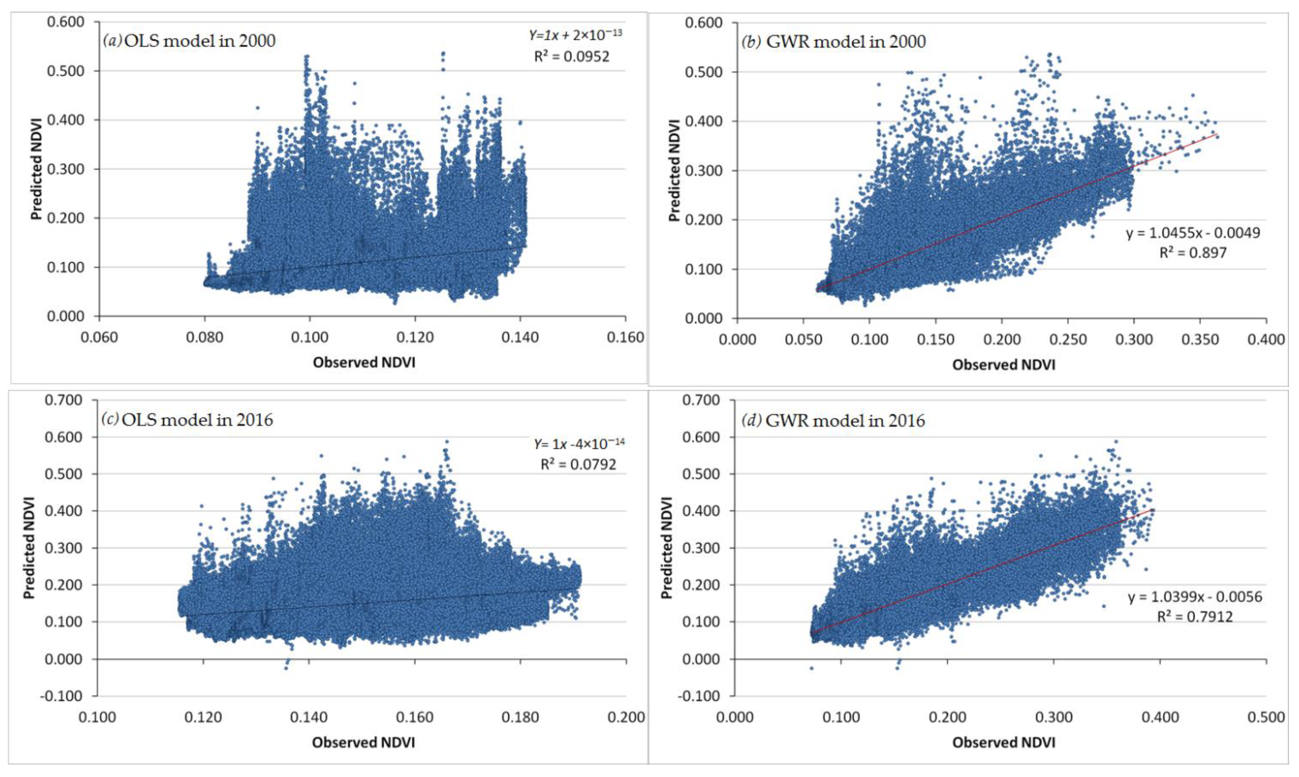
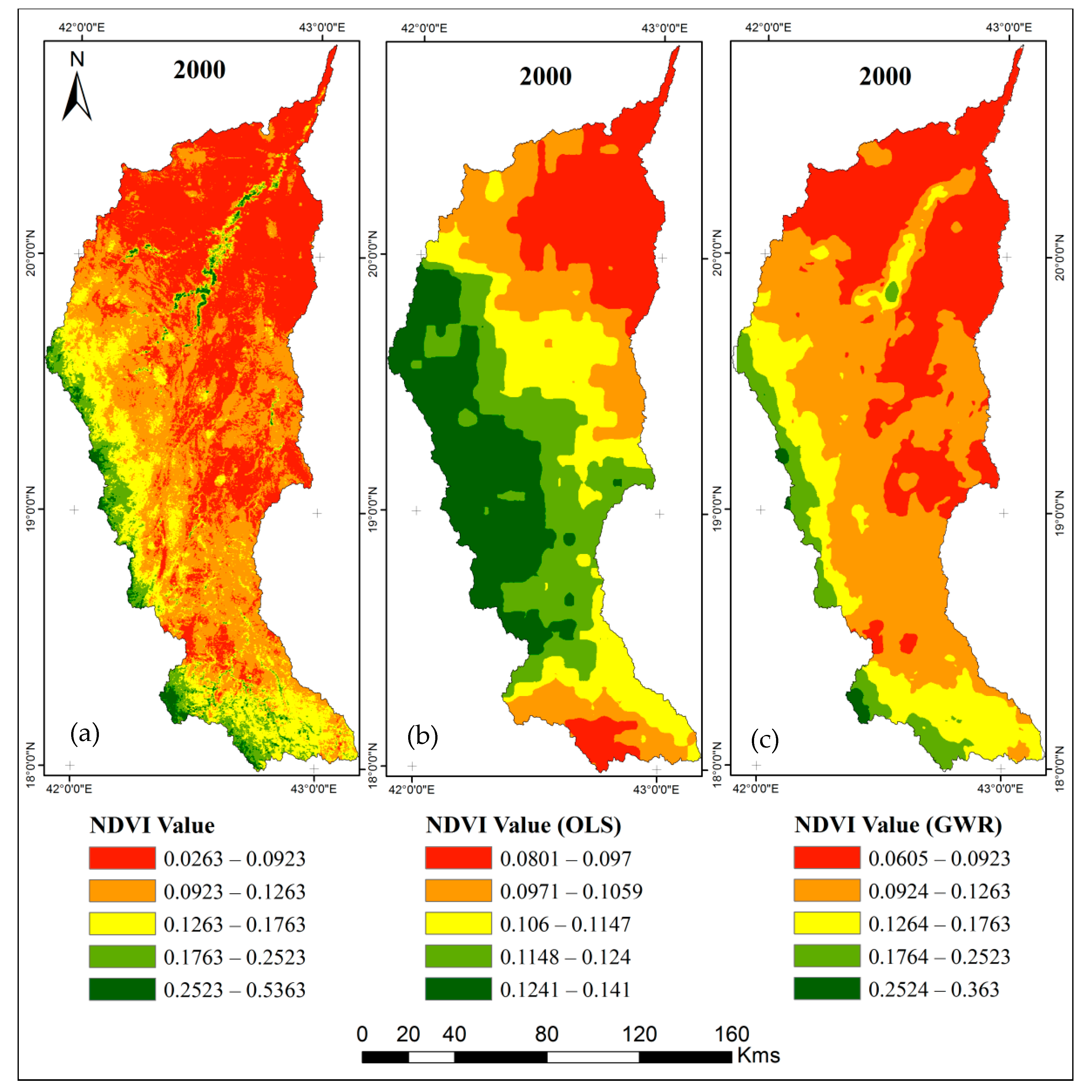
For NDVI datasets of two years, the output of rainfall based on global and local models, namely OLS and GWR, calculated using MAE and RMSE, as presented in Table 2. It indicates that the GWR model promoted better than the OLS model for each of the study’s years. Figure 8 depicts the scatterplots of predicted and observed values from the OLS and GWR models in 2000 and 2016. Since, the constant collection of variables has been used to construct a relationship over a substantial area with high spatial variability. Moreover, it generates a single regression equation to describe the procedure, and the OLS global models overpredicted the NDVI values. The GWR’s local modeling methodology was able to achieve more reliable results by integrating the local characteristics. Figure 9 and Figure 10 represent observed and projected NDVI spatial patterns for the years 2000 and 2016. The OLS model developed more generalized trends in the NDVI across the watershed, ignoring local geographic variability (RMSE 0.041 and MAE 0.165 in 2000; RMSE 0.025 and MAE 0.017 in 2016 ). The GWR local model (Table 2), on the other hand, was more reliable because it took into account local spatial variability (RMSE 0.021 and MAE 0.09 in 2000; RMSE 0.0525 and MAE 0.198 in 2016) and other ecological variables in the NDVI–rainfall relationship.
The results showed that during the rainy season (March to June) in 2000 and 2016, the NDVI–rainfall relationship was non-stationary over the Bisha watershed. The study found that rainfall is an important good predictor of NDVI when spatial non-stationarity is included in the regression model. Across the majority of the study area, the coefficient relationship was positive. Some patches, on the other hand, have very weak or negative relationships. Furthermore, the significance of association varied depending on the study area. When compared to global OLS models, GWR is a method that identifies a continuous variant in spatial relationships by integrating local information with significantly better efficiency.

4. Discussion

During the growing season in the years 2000 and 2016, the NDVI–rainfall relationship was non-stationary in the Bisha watershed. As a result, describing the relationship as a set of spatially constant coefficients is illogical. Foody [53] investigated the spatial variability of rainfall and NDVI in semi-arid and arid climate settings in northern Africa. The relationship was positive in that study, but this can be interpreted by the different datasets used (MODIS and CHIRPS datasets). In this analysis, the majority of the study region had a positive relationship, but some areas had negative or very bad relationships as well. Furthermore, the importance of the relationship changed substantially.
Regression and spatial distribution of coefficient results showed that the gradual transition from arid and semi-arid regions to more humid regions was one factor. Along with transition zones between semi-arid and wet environments, significant locations for the growing season were identified that were very sensitive to changes in cumulative rainfall. Zhao et al. [49] found that the transition region between deserts and humid lands in North China tended to be more susceptible to climatic changes than areas surrounding it, and the same finding was also reflected in the study of Georganos et al., [37] in the Sahel northern Africa.
“According to the analysis, temporal variability was noticed in their spatial relationships, as 2000 was a reasonably dry year, whereas 2016 was a rainy year. Despite a decade of temporal discontinuity in the results, the assumption is that the rainfall quantity obtained in each region in a given timeframe is essential for the output of the results. In comparison to 2016, higher local fits and rainfall coefficients were observed in 2000. When rainfall is low, its influence as a predictor variable and the resilience of vegetation to it tend to be greater than in rainfall years. Furthermore, some areas in 2016 produced exceptionally high slope coefficients, exceeding even the highest slope coefficients in 2000. This may be due to a change in land cover, a difference in irrigation practices, or an uncertainty about the data’s accuracy and validity. Regardless, GWR has shown its ability to provide local areas of interest that can direct future research and improve the modeling of phenomena in these regions.
Between variance in local estimates and model preconceptions, the bandwidth selection is a substitute. In general, AICc is used to make this decision, however, with large sample sizes, AICc can indicate optimal situations in models with very narrow bandwidth, miscalculated R2 values with high standard errors [75]. It also avoids significant interpretations and adds a lot of noise into the data. Once the required bandwidth is allocated based on the Stationarity index, AICc is ideal for comparing GWR and OLS in the current analysis (SI). Though, it is important to keep in mind that in bivariate models with a broad sample size (n > 10,000) and very high collinearity problems (unstable and difficult to interpret coefficient estimates) are likely to occur in local exploratory relationships. In the Bisha watershed rainfall season, the SI estimation at expanding spatial scales interprets sufficient information related to the the bandwidth dependence of NDVI and rainfall. The two-year dataset chosen, based on the occurrence of high and low rainfall, for detailed analysis, exhibited that SI stabilized at 12000 meters (Figure 2). The regressions were more consistent and stable at that bandwidth. Local correlation coefficients and condition variables showed no bias in the local correlation.
In heterogeneous areas that are susceptible to landscape ecology changes, the study showed that GWR could be a viable alternative to OLS modeling. Using the local method, the predictions were higher, and residual autocorrelation was lower. In addition, interesting local trends were highlighted. Since rainfall and NDVI relationships are spatially varying, the outcomes of this study can be used to model a net primary product in the Bisha watershed as a function of space. In the Net primary model (NPM) models, both NDVI and rainfall are common components, and their interactions can differ locally [52]. In addition to that, in a heterogeneous setting like the Bisha watershed, it may also be used as a tool for estimating juniper woodlands biomass if linear regression is insufficient to capture the true relationship. Finally, GWR analysis using data from various satellite sources may help us better understand the impact of data spatial resolution on the estimated relationships between vegetation and climatic variables.
The study established that the NDVI–rainfall relationship is non-stationary. This means that modeling this relationship using global or stratified OLS regression produces highly uncertain results. The variation in the relationship across the study region’s space is explained by the variation in underlying environmental factors such as vegetation composition, soil type, hydrology, and land use caused by the terrain’s diversity. This is consistent with the findings from other regions on vegetation–climate relationships [35,36]. Another way to get similar results would be to classify the Bisha watershed into geographical regions that have the same characteristics as was seen in research done by Zhao et al., [51] in Northern China. However, it will be very time-consuming and uneconomical since there is a huge amount of data to deal with from both a spatial and temporal context. Thus, GWR is recommended as an explanatory and exploratory technique when relations between variables are subject to spatial variability.

Limitation of the Study

In this study, two statistical methods are used in the modeling, i.e., traditional OLS regression and GWR, to evaluate the NDVI–rainfall relationship. Indeed, most of the aspects introduced in this study are well-known to geostatistics experts and have been explored in geostatistical methods for many years. Though, in the international literature on ecology and environmental science, local regression models have not yet gained widespread acceptance (see, for example, the scientific work on local regression methods by Jetz et al. [76], Propastin et al. [77], and Georganos et al. [37]). As a result, the authors of these papers did not set out to innovate in the area of geostatistical data analysis techniques. Rather than that, this study should be viewed as a contribution to the ongoing debate in ecology and environmental science about local and global approaches to spatial data analysis. The study’s findings should be used to further model primary production and its relationship to environmental factors in the phytogeographic region called the Afromontane, which is part of the watershed area.
In analyzing the relationship between NDVI trends and rainfall, our analysis demonstrated the superiority of GWR’s local approach over the global OLS approach. This superiority stems primarily from the consideration of the relationship’s spatial variance across the study area. Global regression techniques such as OLS can overlook local details, implying that a significant portion of the NDVI variance is unaccounted for. Since the GWR is a local form of spatial analysis that aligned to local conditions, it has the potential for more accurate prediction. Still, a more significant number of data is needed to enable a reliable local fitting, such as terrain, vegetation species, soil, and air temperature related to climate change. The method proposed in this paper should be investigated further by adding additional variables such as topographic characteristics such as slope, flow accumulation area, flow direction, aspect, and topographic index, and other biophysical parameters, i.e., vegetation species, soil, and air temperature. Since this result has been validated/compared with the LST product of the MODIS (MOD11A1v006) under a particular set of environmental conditions (arid, semi-arid), further field work, temperature data, and LST measurements from other satellite data such as LANDSAT-8 and Sentinel are required to further extend this approach to a broader set of environmental conditions.

5. Conclusions

This study aims to evaluate the relationship between NDVI and rainfall variability in the semi-arid Bisha watershed in Saudi Arabia by a non-stationary modeling technique. Cumulative rainfall data, March to June, for the months of March to June (2000 and 2016) was calculated using CHIRPS. In the GWR, variables use a methodology in which the contribution of the sample to the analysis is weighted by its proximity to the geographic region of interest. As a result of this, the weighting of observation does not remain constant in the calibration.“ The GWR uses models to generate the maps of slope parameters local R2, (β coefficients), and standardized residuals (StdResid) to illustrate the spatial variability relationships between suitable bandwidth and related variables. The coefficient of determination (R2) for GWR was significantly higher than the model produced with the OLS method both years (2000 and 2016). The findings validated the initial hypothesis, which was that GWR local modeling is a viable alternative to OLS global modeling in heterogeneous areas that are instability to ecosystems.
In the years 2000 and 2016, the analysis found that the NDVI–rainfall relationship is non-stationary over the Bisha watershed during the rainy months (March–June). If spatial non-stationarity can be incorporated into the regression model, the finding suggests that rainfall is indeed a significantly powerful predictor of NDVI. Across the majority of the study region, the coefficient relationship was positive. Some patches, on the other hand, have very weak or negative relationships. Furthermore, the significance of association varied depending on the study region. Compared to global OLS models, GWR is a method that identifies continuous variation in spatial relationships by integrating local information with significantly better efficiency. It has been found that certain areas in the study area were significantly more susceptible to changes in rainfall, which resulted in the creation of numerous interconnected clusters that linked arid and wet zones. It appears that rainfall is the most significant factor in deciding the distribution of vegetation in these regions. Furthermore, rainfall had weak relationships with regions predominantly located around wetlands, suggesting the need for additional factors to describe NDVI variations. When using the GWR method, predictions were higher, with lower autocorrelation in the residuals, and interesting local variations became evident. Thus, GWR is recommended as an explanatory and exploratory technique when relations between variables are subject to spatial variability.

Author Contributions

Conceptualization, J.M., M.K.A., V.P.S., and I.I.F.; formal analysis, J.M., I.I.F., C.K.S., and N.B.K.; funding acquisition, J.M.; investigation, V.P.S. and C.K.S.; methodology, J.M., M.K.A., and M.A.; project administration, M.K.A. and I.I.F.; resources, M.K.A., V.P.S., I.I.F., M.A., and N.B.K.; software, J.M.; supervision, M.K.A., V.P.S., and N.B.K.; writing—original draft, J.M and M.K.A.; writing—review and editing, V.P.S. and C.K.S. All authors have read and agreed to the published version of the manuscript.

Funding

Funding for this research was given under award numbers 669 by the deputyship for Research & Innovation, Ministry of Education in Saudi Arabia.

Institutional Review Board Statement

Not applicable.

Informed Consent Statement

Not applicable.

Data Availability Statement

Data availability on request.

Conflicts of Interest

The authors declare no conflict of interest.

References

  1. Nanzad, L.; Zhang, J.; Tuvdendorj, B.; Nabil, M.; Zhang, S.; Bai, Y. NDVI anomaly for drought monitoring and its correlation with climate factors over Mongolia from 2000 to 2016. J. Arid Environ. 2019, 164, 69–77. [Google Scholar] [CrossRef]
  2. Lu, J.; Carbone, G.J.; Gao, P. Mapping the agricultural drought based on the long-term AVHRR NDVI and North American Regional Reanalysis (NARR) in the United States, 1981–2013. Appl. Geogr. 2019, 104, 10–20. [Google Scholar] [CrossRef]
  3. Quarmby, N.A.; Milnes, M.; Hindle, T.L.; Silleos, N. The use of multi-temporal NDVI measurements from AVHRR data for crop yield estimation and prediction. Int. J. Remote Sens. 1993, 14, 199–210. [Google Scholar] [CrossRef]
  4. Huang, J.; Wang, H.; Dai, Q.; Han, D. Analysis of NDVI data for crop identification and yield estimation. IEEE J. Sel. Top. Appl. Earth Obs. Remote Sens. 2014, 7, 4374–4384. [Google Scholar] [CrossRef]
  5. Heumann, B.W.; Seaquist, J.W.; Eklundh, L.; Jönsson, P. AVHRR derived phenological change in the Sahel and Soudan, Africa, 1982–2005. Remote Sens. Environ. 2007, 108, 385–392. [Google Scholar] [CrossRef]
  6. Pereira Coltri, P.; Zullo, J.; Ribeiro Do Valle Goncalves, R.; Romani, L.A.S.; Pinto, H.S. Coffee crop’s biomass and carbon stock estimation with usage of high resolution satellites images. IEEE J. Sel. Top. Appl. Earth Obs. Remote Sens. 2013, 6, 1786–1795. [Google Scholar] [CrossRef]
  7. Liu, B.; Chen, J.; Chen, J.; Zhang, W. Land Cover Change Detection Using Multiple Shape Parameters of Spectral and NDVI Curves. Remote Sens. 2018, 10, 1251. [Google Scholar] [CrossRef] [Green Version]
  8. Lunetta, R.S.; Knight, J.F.; Ediriwickrema, J.; Lyon, J.G.; Worthy, L.D. Land-cover change detection using multi-temporal MODIS NDVI data. Remote Sens. Environ. 2006, 105, 142–154. [Google Scholar] [CrossRef]
  9. Tadesse, T.; Brown, J.F.; Hayes, M.J. A New Approach for Predicting Drought-Related Vegetation Stress: Integrating Satellite, Climate, and Biophysical Data over the U.S. Central Plains. ISPRS J. Photogramm. Remote Sens. 2005, 59, 244–253. [Google Scholar] [CrossRef]
  10. Song, X.; Saito, G.; Kodama, M.; Sawada, H. Early detection system of drought in East Asia using NDVI from NOAA/AVHRR data. Int. J. Remote Sens. 2004, 25, 3105–3111. [Google Scholar] [CrossRef] [Green Version]
  11. Kogan, F.N. Global Drought Watch from Space. Bull. Am. Meteorol. Soc. 1997, 78, 621–636. [Google Scholar] [CrossRef]
  12. Kawabata, A.; Ichii, K.; Yamaguchi, Y. Global monitoring of interannual changes in vegetation activities using NDVI and its relationships to temperature and precipitation. Int. J. Remote Sens. 2001, 22, 1377–1382. [Google Scholar] [CrossRef]
  13. Potter, C.S.; Brooks, V. Global analysis of empirical relations between annual climate and seasonality of NDVI. Int. J. Remote Sens. 1998, 19, 2921–2948. [Google Scholar] [CrossRef]
  14. Nezlin, N.P.; Kostianoy, A.G.; Li, B.L. Inter-annual variability and interaction of remote-sensed vegetation index and atmospheric precipitation in the Aral Sea region. J. Arid Environ. 2005, 62, 677–700. [Google Scholar] [CrossRef]
  15. Evans, J.; Geerken, R. Discrimination between climate and human-induced dryland degradation. J. Arid Environ. 2004, 57, 535–554. [Google Scholar] [CrossRef]
  16. Li, J.; Lewis, J.; Rowland, J.; Tappan, G.; Tieszen, L. Evaluation of land performance in Senegal using multi-temporal NDVI and rainfall series. J. Arid Environ. 2004, 59, 463–480. [Google Scholar] [CrossRef]
  17. Budde, M.; Tappan, G.; Rowland, J.; Lewis, J.; Tieszen, L. Assessing land cover performance in Senegal, West Africa using 1-km integrated NDVI and local variance analysis. J. Arid Environ. 2004, 59, 481–498. [Google Scholar] [CrossRef]
  18. Weiss, E.; Marsh, S.E.; Pfirman, E.S. Application of NOAA-AVHRR NDVI time-series data to assess changes in Saudi Arabia’s rangelands. Int. J. Remote Sens. 2001, 22, 1005–1027. [Google Scholar] [CrossRef]
  19. Xiao, J.; Moody, A. Trends in vegetation activity and their climatic correlates: China 1982 to 1998. Int. J. Remote Sens. 2004, 25, 5669–5689. [Google Scholar] [CrossRef]
  20. Tucker, C.J.; Slayback, D.A.; Pinzon, J.E.; Los, S.O.; Myneni, R.B.; Taylor, M.G. Higher northern latitude normalized difference vegetation index and growing season trends from 1982 to 1999. Int. J. Biometeorol. 2001, 45, 184–190. [Google Scholar] [CrossRef]
  21. Amini, A.; Abdeh Kolahchi, A.; Al-Ansari, N.; Karami Moghadam, M.; Mohammad, T. Application of TRMM Precipitation Data to Evaluate Drought and Its Effects on Water Resources Instability. Appl. Sci. 2019, 9, 5377. [Google Scholar] [CrossRef] [Green Version]
  22. Funk, C.; Peterson, P.; Landsfeld, M.; Pedreros, D.; Verdin, J.; Shukla, S.; Husak, G.; Rowland, J.; Harrison, L.; Hoell, A.; et al. The climate hazards infrared precipitation with stations—A new environmental record for monitoring extremes. Sci. Data 2015, 2, 1–21. [Google Scholar] [CrossRef] [Green Version]
  23. Paredes Trejo, F.J.; Barbosa, H.A.; Peñaloza-Murillo, M.A.; Alejandra Moreno, M.; Farías, A. Intercomparison of improved satellite rainfall estimation with CHIRPS gridded product and rain gauge data over Venezuela. Atmosfera 2016, 29, 323–342. [Google Scholar] [CrossRef] [Green Version]
  24. Toté, C.; Patricio, D.; Boogaard, H.; van der Wijngaart, R.; Tarnavsky, E.; Funk, C. Evaluation of Satellite Rainfall Estimates for Drought and Flood Monitoring in Mozambique. Remote Sens. 2015, 7, 1758–1776. [Google Scholar] [CrossRef] [Green Version]
  25. Ebert, E.E.; Janowiak, J.E.; Kidd, C. Comparison of near-real-time precipitation estimates from satellite observations and numerical models. Bull. Am. Meteorol. Soc. 2007, 88, 47–64. [Google Scholar] [CrossRef] [Green Version]
  26. Dinku, T.; Ruiz, F.; Connor, S.J.; Ceccato, P. Validation and intercomparison of satellite rainfall estimates over Colombia. J. Appl. Meteorol. Climatol. 2010, 49, 1004–1014. [Google Scholar] [CrossRef]
  27. Nicholson, S.E.; Some, B.; McCollum, J.; Nelkin, E.; Klotter, D.; Berte, Y.; Diallo, B.M.; Gaye, I.; Kpabeba, G.; Ndiaye, O.; et al. Validation of TRMM and other rainfall estimates with a high-density gauge dataset for West Africa. Part II: Validation of TRMM rainfall products. J. Appl. Meteorol. 2003, 42, 1355–1368. [Google Scholar] [CrossRef]
  28. Laurent, H.; Jobard, I.; Toma, A. Validation of satellite and ground-based estimates of precipitation over the Sahel. Atmos. Res. 1998, 47–48, 651–670. [Google Scholar] [CrossRef]
  29. Franchito, S.H.; Rao, V.B.; Vasques, A.C.; Santo, C.M.E.; Conforte, J.C. Validation of TRMM precipitation radar monthly rainfall estimates over Brazil. J. Geophys. Res. 2009, 114, D02105. [Google Scholar] [CrossRef] [Green Version]
  30. Mallick, J.; Singh, R.K.; Khan, R.A.; Singh, C.K.; Kahla, N.B.; Warrag, E.I.; Islam, S.; Rahman, A. Examining the rainfall–topography relationship using non-stationary modelling technique in semi-arid Aseer region, Saudi Arabia. Arab. J. Geosci. 2018, 11, 1–16. [Google Scholar] [CrossRef]
  31. Bai, L.; Shi, C.; Li, L.; Yang, Y.; Wu, J. Accuracy of CHIRPS satellite-rainfall products over mainland China. Remote Sens. 2018, 10, 362. [Google Scholar] [CrossRef] [Green Version]
  32. Wang, J.; Price, K.P.; Rich, P.M. Spatial patterns of NDVI in response to precipitation and temperature in the central Great Plains. Int. J. Remote Sens. 2001, 22, 3827–3844. [Google Scholar] [CrossRef]
  33. Farrar, T.J.; Nicholson, S.E.; Lare, A.R. The influence of soil type on the relationships between NDVI, rainfall, and soil moisture in semiarid Botswana. II. NDVI response to soil oisture. Remote Sens. Environ. 1994, 50, 121–133. [Google Scholar] [CrossRef]
  34. Richard, Y.; Poccard, I. A statistical study of NDVI sensitivity to seasonal and interannual rainfall variations in Southern Africa. Int. J. Remote Sens. 1998, 19, 2907–2920. [Google Scholar] [CrossRef]
  35. Ji, L.; Peters, A.J. A spatial regression procedure for evaluating the relationship between AVHRR-NDVI and climate in the northern Great Plains. Int. J. Remote Sens. 2004, 25, 297–311. [Google Scholar] [CrossRef]
  36. Yang, L.; Wylie, B.K.; Tieszen, L.L.; Reed, B.C. An analysis of relationships among climate forcing and time-integrated NDVI of grasslands over the U.S. northern and central Great Plains. Remote Sens. Environ. 1998, 65, 25–37. [Google Scholar] [CrossRef]
  37. Georganos, S.; Abdi, A.M.; Tenenbaum, D.E.; Kalogirou, S. Examining the NDVI-rainfall relationship in the semi-arid Sahel using geographically weighted regression. J. Arid Environ. 2017, 146, 64–74. [Google Scholar] [CrossRef]
  38. Wang, T.; Kou, X.; Xiong, Y.; Mou, P.; Wu, J.; Ge, J. Temporal and spatial patterns of NDVI and their relationship to precipitation in the loess plateau of China. Int. J. Remote Sens. 2010, 31, 1943–1958. [Google Scholar] [CrossRef]
  39. Udelhoven, T.; Stellmes, M.; del Barrio, G.; Hill, J. Assessment of rainfall and NDVI anomalies in Spain (1989-1999) using distributed lag models. Int. J. Remote Sens. 2009, 30, 1961–1976. [Google Scholar] [CrossRef]
  40. Fabricante, I.; Oesterheld, M.; Paruelo, J.M. Annual and seasonal variation of NDVI explained by current and previous precipitation across Northern Patagonia. J. Arid Environ. 2009, 73, 745–753. [Google Scholar] [CrossRef]
  41. Huber, S.; Fensholt, R.; Rasmussen, K. Water availability as the driver of vegetation dynamics in the African Sahel from 1982 to 2007. Glob. Planet. Chang. 2011, 76, 186–195. [Google Scholar] [CrossRef]
  42. Martiny, N.; Camberlin, P.; Richard, Y.; Philippon, N. Compared regimes of NDVI and rainfall in semi-arid regions of Africa. Int. J. Remote Sens. 2006, 27, 5201–5223. [Google Scholar] [CrossRef]
  43. Kang, L.; Di, L.; Deng, M.; Shao, Y.; Yu, G.; Shrestha, R. Use of geographically weighted regression model for exploring spatial patterns and local factors behind NDVI-precipitation correlation. IEEE J. Sel. Top. Appl. Earth Obs. Remote Sens. 2014, 7, 4530–4538. [Google Scholar] [CrossRef]
  44. McMillen, D.P. Geographically Weighted Regression: The Analysis of Spatially Varying Relationships. Am. J. Agric. Econ. 2004, 86, 554–556. [Google Scholar] [CrossRef]
  45. Stewart Fotheringham, A.; Charlton, M.; Brunsdon, C. The geography of parameter space: An investigation of spatial non-stationarity. Int. J. Geogr. Inf. Syst. 1996, 10, 605–627. [Google Scholar] [CrossRef]
  46. Brunsdon, C.; Fotheringham, A.S.; Charlton, M.E. Geographically Weighted Regression: A Method for Exploring Spatial Nonstationarity. Geogr. Anal. 2010, 28, 281–298. [Google Scholar] [CrossRef]
  47. Cahill, M.; Mulligan, G. Using Geographically Weighted Regression to Explore Local Crime Patterns. Soc. Sci. Comput. Rev. 2007, 25, 174–193. [Google Scholar] [CrossRef]
  48. Hu, M.; Li, Z.; Wang, J.; Jia, L.; Liao, Y.; Lai, S.; Guo, Y.; Zhao, D.; Yang, W. Determinants of the Incidence of Hand, Foot and Mouth Disease in China Using Geographically Weighted Regression Models. PLoS ONE 2012, 7, e38978. [Google Scholar] [CrossRef] [PubMed]
  49. Zhao, Z.; Gao, J.; Wang, Y.; Liu, J.; Li, S. Exploring spatially variable relationships between NDVI and climatic factors in a transition zone using geographically weighted regression. Theor. Appl. Climatol. 2015, 120, 507–519. [Google Scholar] [CrossRef]
  50. Gaughan, A.E.; Waylen, P.R. Spatial and temporal precipitation variability in the Okavango-Kwando-Zambezi catchment, southern Africa. J. Arid Environ. 2012, 82, 19–30. [Google Scholar] [CrossRef]
  51. Wang, Q.; Ni, J.; Tenhunen, J. Application of a geographically-weighted regression analysis to estimate net primary production of Chinese forest ecosystems. Glob. Ecol. Biogeogr. 2005, 14, 379–393. [Google Scholar] [CrossRef]
  52. Foody, G.M. Spatial nonstationarity and scale-dependency in the relationship between species richness and environmental determinants for the sub-Saharan endemic avifauna. Glob. Ecol. Biogeogr. 2004, 13, 315–320. [Google Scholar] [CrossRef]
  53. Foody, G.M. Geographical weighting as a further refinement to regression modelling: An example focused on the NDVI-rainfall relationship. Remote Sens. Environ. 2003, 88, 283–293. [Google Scholar] [CrossRef]
  54. Peter Vincent Saudi Arabia: An Environmental Overview—1st Edition. Available online: https://www.routledge.com/Saudi-Arabia-An-Environmental-Overview/Vincent/p/book/9780367387815 (accessed on 16 March 2021).
  55. Al-Ahmadi, K.; Al-Ahmadi, S. Rainfall-altitude relationship in Saudi Arabia. Adv. Meteorol. 2013, 2013. [Google Scholar] [CrossRef]
  56. Peel, M.C.; Finlayson, B.L.; McMahon, T.A. Updated world map of the Köppen-Geiger climate classification. Hydrol. Earth Syst. Sci. 2007, 11, 1633–1644. [Google Scholar] [CrossRef] [Green Version]
  57. Kottek, M.; Grieser, J.; Beck, C.; Rudolf, B.; Rubel, F. World map of the Köppen-Geiger climate classification updated. Meteorol. Z. 2006, 15, 259–263. [Google Scholar] [CrossRef]
  58. Wu, Y.L.; Li, Z.C.; Wang, Y.F.; Luan, Q.; Tian, G.Z. Responses of Vegetation Index (NDVI) in Typical Ecological Areas of Shanxi Province to Climate Change. Available online: http://www.cje.net.cn/EN/abstract/abstract15343.shtml (accessed on 16 March 2021).
  59. Gong, Z.; Zhao, S.; Gu, J. Correlation analysis between vegetation coverage and climate drought conditions in North China during 2001–2013. J. Geogr. Sci. 2017, 27, 143–160. [Google Scholar] [CrossRef]
  60. Mallick, J.; Talukdar, S.; Alsubih, M.; Salam, R.; Ahmed, M.; Kahla, N.B.; Shamimuzzaman, M. Analysing the trend of rainfall in Asir region of Saudi Arabia using the family of Mann-Kendall tests, innovative trend analysis, and detrended fluctuation analysis. Theor. Appl. Climatol. 2021, 143, 823–841. [Google Scholar] [CrossRef]
  61. Wheater, H.S.; Laurentis, P.; Hamilton, G.S. Design Rainfall Characteristics for South-West Saudi Arabia. Proc. Inst. Civ. Eng. 1989, 87, 517–538. [Google Scholar] [CrossRef]
  62. Baillie, J.E.M.; Groombridge, B. IUCN Red List of Threatened Species. Available online: https://www.iucnredlist.org/resources/baillie1996 (accessed on 16 March 2021).
  63. Davis, S.D.; Heywood, V. Centres of Plant Diversity: A Guide and Strategy for Their Conservation, v.1. Europe, Africa, South West Asia and the Middle East | IUCN. Available online: https://www.iucn.org/content/centres-plant-diversity-a-guide-and-strategy-their-conservation-v1-europe-africa-south-west-asia-and-middle-east (accessed on 16 March 2021).
  64. Hosni, H.A.; Hegazy, A.K. Contribution to the flora of Asir, Saudi Arabia. Candollea 1996, 51, 169–202. [Google Scholar]
  65. Fensholt, R.; Proud, S.R. Evaluation of Earth Observation based global long term vegetation trends—Comparing GIMMS and MODIS global NDVI time series. Remote Sens. Environ. 2012, 119, 131–147. [Google Scholar] [CrossRef]
  66. Zhu, A.-X. Resampling, Raster. In International Encyclopedia of Geography: People, The Earth, Environment and Technology; John Wiley & Sons, Ltd.: Oxford, UK, 2017; pp. 1–5. [Google Scholar]
  67. Behnke, R.; Vavrus, S.; Allstadt, A.; Albright, T.; Thogmartin, W.E.; Radeloff, V.C. Evaluation of downscaled, gridded climate data for the conterminous United States. Ecol. Appl. 2016, 26, 1338–1351. [Google Scholar] [CrossRef] [PubMed]
  68. Kalogirou, S. The Statistical Analysis and Modelling of Internal Migration Flows within England and Wales by Stamatis Kalogirou. Ph.D. Thesis, Newcastle University, Newcastle upon Tyne, UK, 2003. [Google Scholar]
  69. Fotheringham, A.S.B. Geographically Weighted Regression; The Analysis of Spatially Varying Relationships | HimalDoc. Available online: https://lib.icimod.org/record/32858 (accessed on 16 March 2021).
  70. Caruso, C.; Quarta, F. Interpolation methods comparison. Comput. Math. Appl. 1998, 35, 109–126. [Google Scholar] [CrossRef] [Green Version]
  71. Dai, X.; Guo, Z.; Zhang, L.; Li, D. Spatio-temporal exploratory analysis of urban surface temperature field in Shanghai, China. Stoch. Environ. Res. Risk Assess. 2010, 24, 247–257. [Google Scholar] [CrossRef]
  72. Xu, S.; Wu, C.; Wang, L.; Gonsamo, A.; Shen, Y.; Niu, Z. A new satellite-based monthly precipitation downscaling algorithm with non-stationary relationship between precipitation and land surface characteristics. Remote Sens. Environ. 2015, 162, 119–140. [Google Scholar] [CrossRef]
  73. Anselin, L. Lagrange Multiplier Test Diagnostics for Spatial Dependence and Spatial Heterogeneity. Geogr. Anal. 2010, 20, 1–17. [Google Scholar] [CrossRef]
  74. Osborne, P.E.; Suárez-Seoane, S. Should data be partitioned spatially before building large-scale distribution models? Ecol. Modell. 2002, 157, 249–259. [Google Scholar] [CrossRef]
  75. Propastin, P.; Kappas, M.; Erasmi, S. Application of Geographically Weighted Regression to Investigate the Impact of Scale on Prediction Uncertainty by Modelling Relationship between Vegetation and Climate. Int. J. Spat. Data Infrastruct. Res. 2008, 3, 73–94. [Google Scholar]
  76. Jetz, W.; Rahbek, C.; Lichstein, J.W. Local and global approaches to spatial data analysis in ecology. Glob. Ecol. Biogeogr. 2005, 14, 97–98. [Google Scholar] [CrossRef]
  77. Propastin, P.A.; Kappas, M. Reducing uncertainty in modeling the NDVI-precipitation relationship: A comparative study using global and local regression techniques. GIScience Remote Sens. 2008, 45, 47–67. [Google Scholar] [CrossRef]
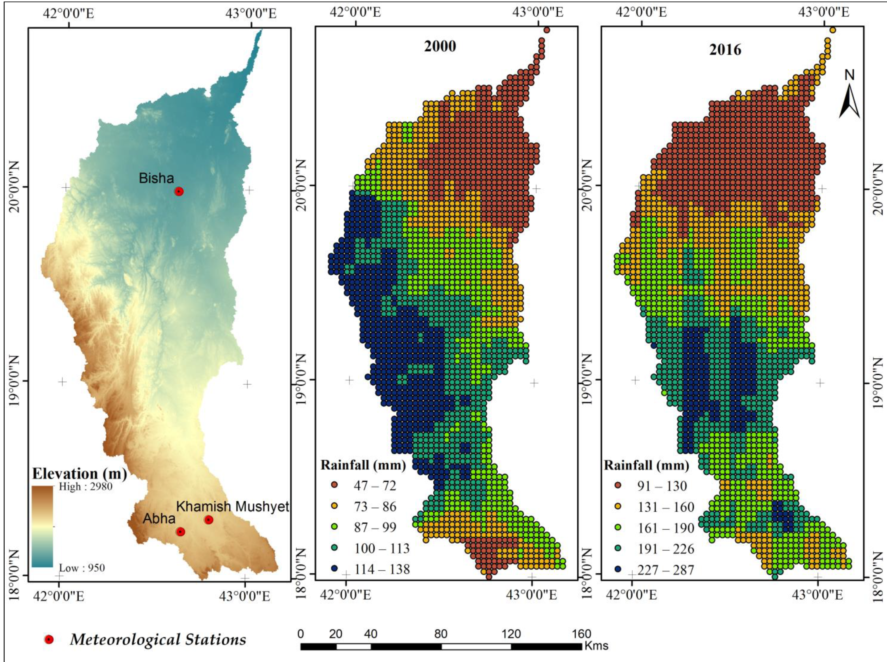
Figure 1. Elevation variability and cumulative rainfall (March–June) trends estimated from “CHIRPS data” in the Bisha watershed for the years 2000 and 2016.
Atmosphere 12 00593 g001
Figure 2. Air temperature statistics from three meteorological stations: (a) Abha; (b) Khamis Mushyet, and (c) Bisha for the years 2000 and 2016 (March–June).
Atmosphere 12 00593 g002
Figure 3. Stationarity index (SI) in 2000 and 2016 at various bandwidths, the SI calculated by the ratio of the interquartile range (IQR) of standard errors (SE) for the geographically weighted regression coefficients with double the SE of a constant.
Atmosphere 12 00593 g003
Figure 4. Rainfall (Beta) coefficient, local R-squared, and Std. residuals in the Bisha watershed for 2000.
Atmosphere 12 00593 g004
Figure 5. Rainfall (Beta) coefficient, local R-squared, and Std. residuals in the Bisha watershed for 2016.
Atmosphere 12 00593 g005
Figure 6. Local Moran’s I index, local Moron’s p-vlaue, and cluster type in the Bisha watershed for 2000 and 2016.
Atmosphere 12 00593 g006
Figure 7. The linear spatio-temporal trends of rainfall coefficients are derived from the differences of rainfall coefficients of 2000 and 2016 over the growing season (March–June).
Atmosphere 12 00593 g007
Figure 8. Observed and predicted NDVI scatter maps of 2000 and 2016: (a) OLS model in 2000; (b) GWR model in 2010; (c) OLS model in 2016; and (d) GWR model in 2016.
Atmosphere 12 00593 g008
Figure 9. Spatial distribution of NDVI in 2000. (a) Observed patterns, (b) global OLS model, (c) GWR model.
Atmosphere 12 00593 g009
Figure 10. Spatial distribution of NDVI in 2016. (a) Observed patterns, (b) global OLS model, (c) GWR model.
Atmosphere 12 00593 g010
Table 1. Statistical summary of CHIRPS datasets product cumulative rainfall (March to June) in mm for the years 2000 and 2016 (as per rainfall intensity).
YearMinimumMaximumMeanMedianSDSkewnessKurtosis
200010.9148.273.469.324.90.44−0.65
201623.2370.8147.7143.042.70.570.48
Table 2. For NDVI datasets from 2000 and 2016, the output of rainfall based on OLS and GWR.
YearModelsRMSE MAE R2
2000Global OLS Model0.041200.16540.095
Local GWR Model0.021190.091000.897
2016Global OLS Model0.052530.19780.079
Local GWR Model0.025080.017120.791
Publisher’s Note: MDPI stays neutral with regard to jurisdictional claims in published maps and institutional affiliations.