
A Multimethod Analysis for Average Annual Precipitation Mapping in the Khorasan Razavi Province (Northeastern Iran)


Abstract
1. Introduction
2. Materials and Methods
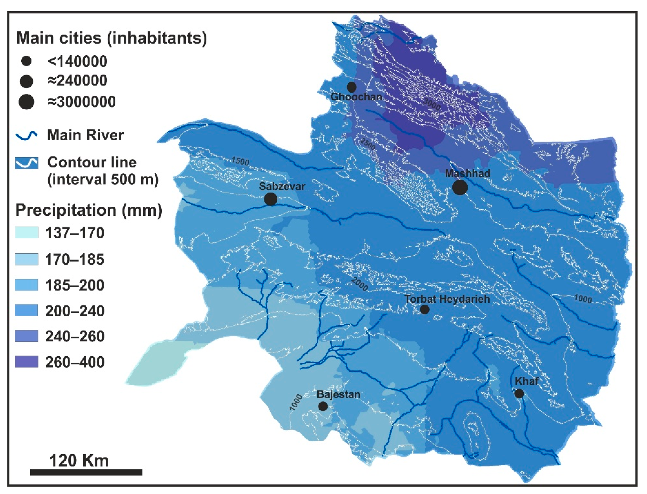
2.1. Study Area and Data Description
2.2. Methods
2.2.1. Inverse Distance Weighting (IDW)
2.2.2. Radial Basis Function (RBF)
2.2.3. Kriging Method
2.2.4. Co-Kriging Method
2.2.5. Non-Linear Regression
2.2.6. Validation Criteria for the Applied Methods
3. Results
3.1. General Statistics
3.2. Interpolation Methods
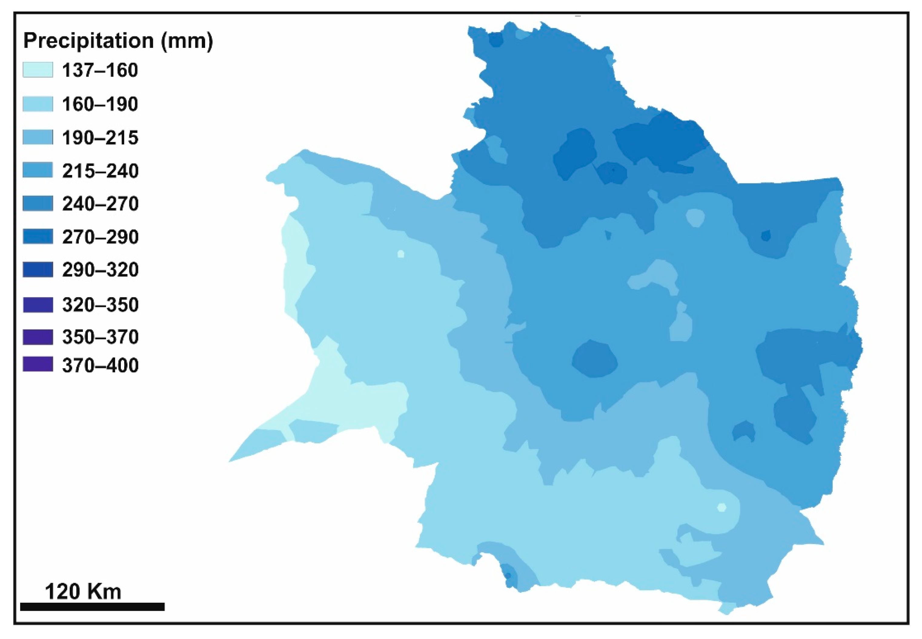
3.2.1. Inverse Distance Weighting (IDW)
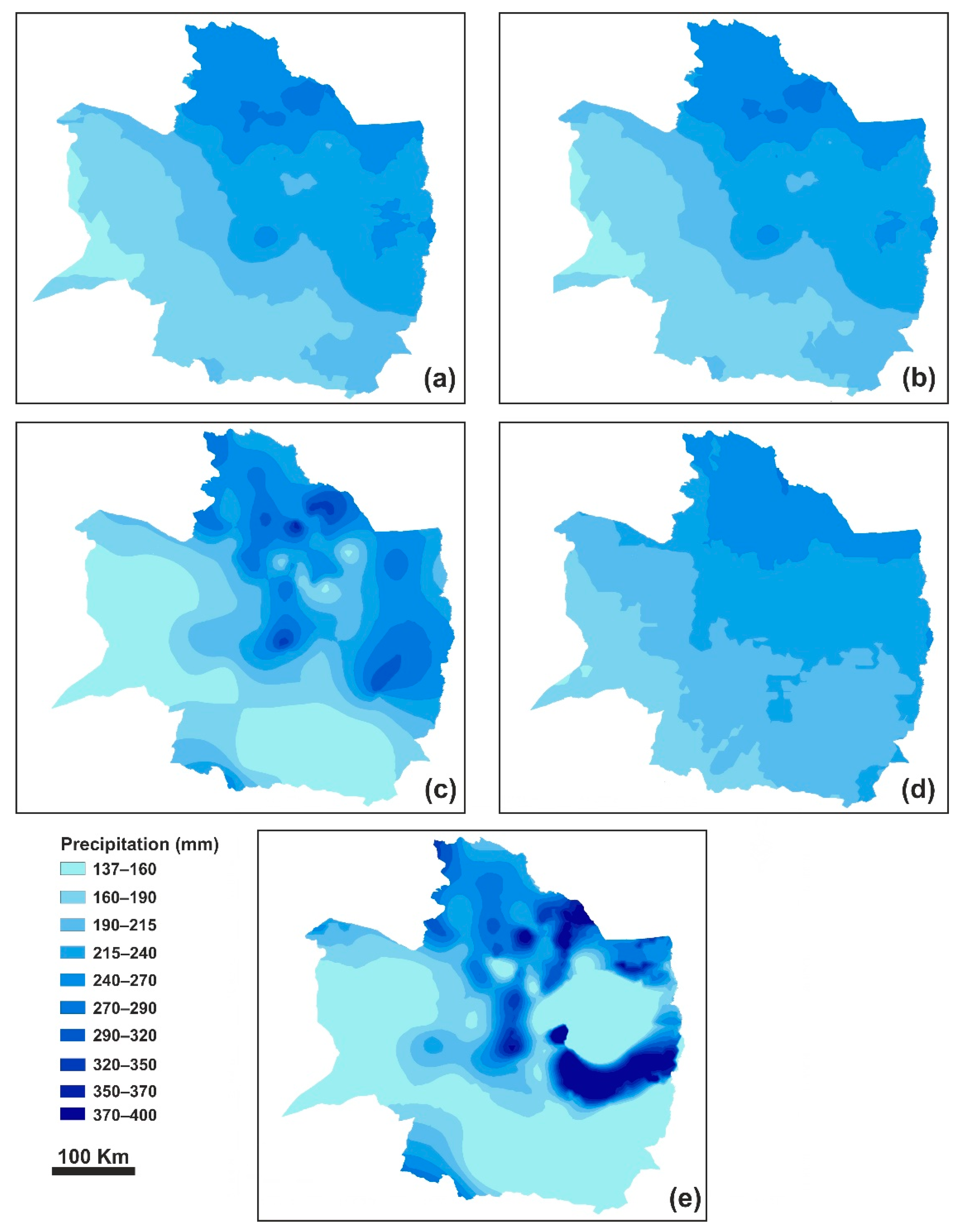
3.2.2. Radial Basis Function (RBF)
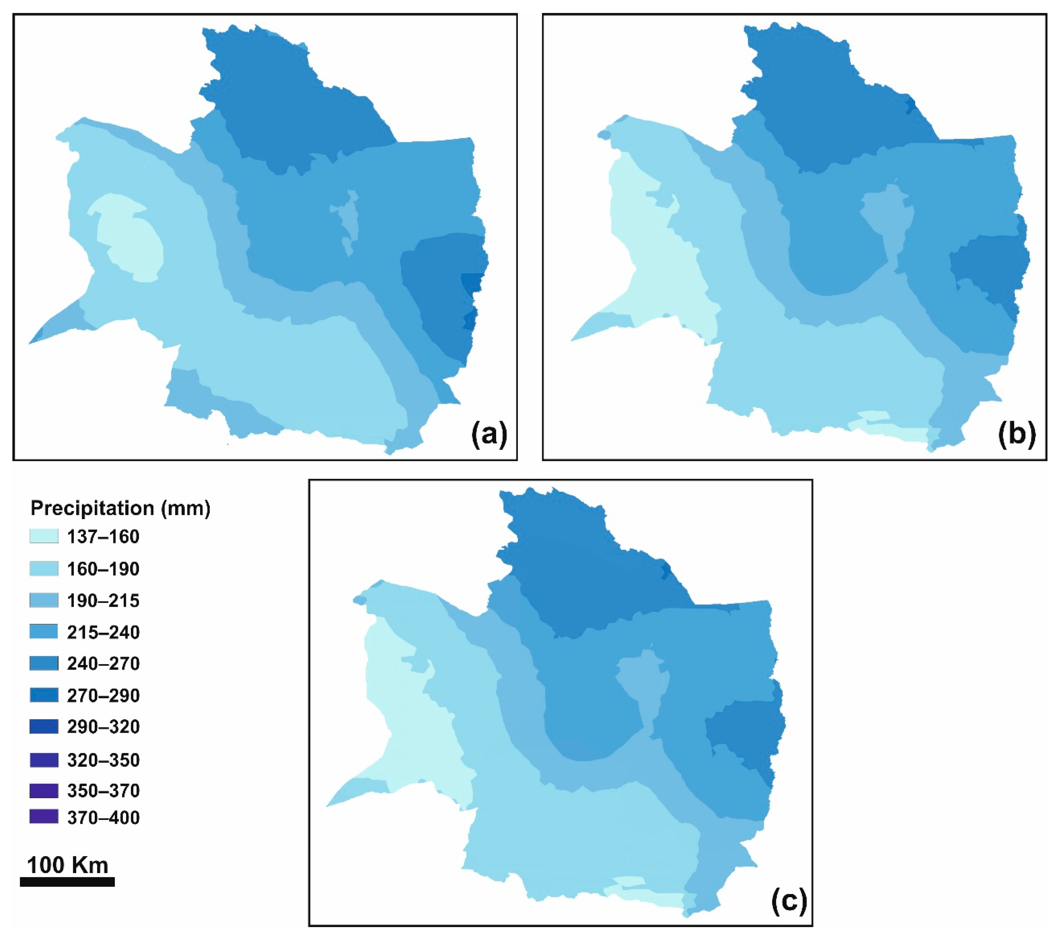
3.2.3. Kriging
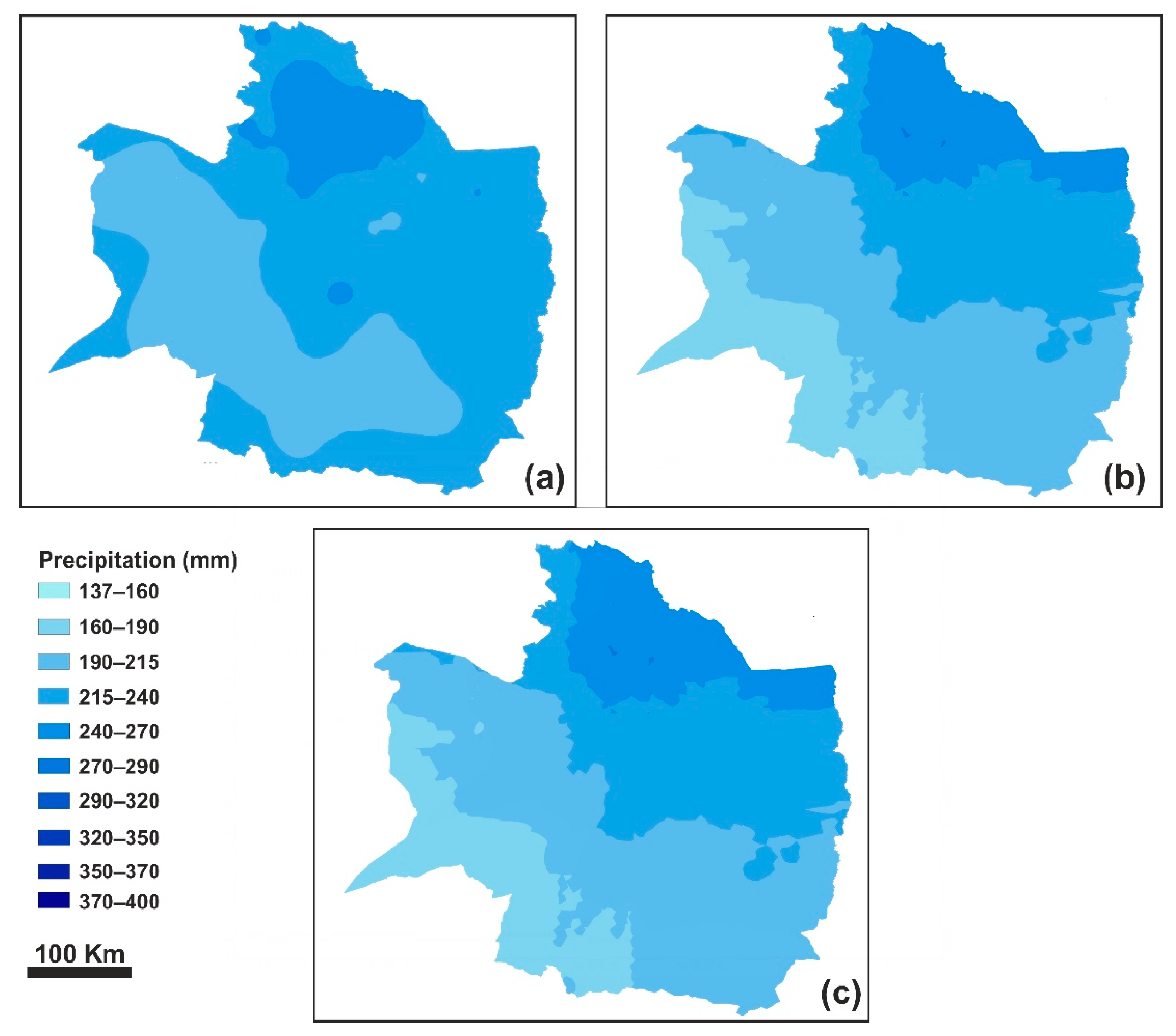
3.2.4. Co-Kriging
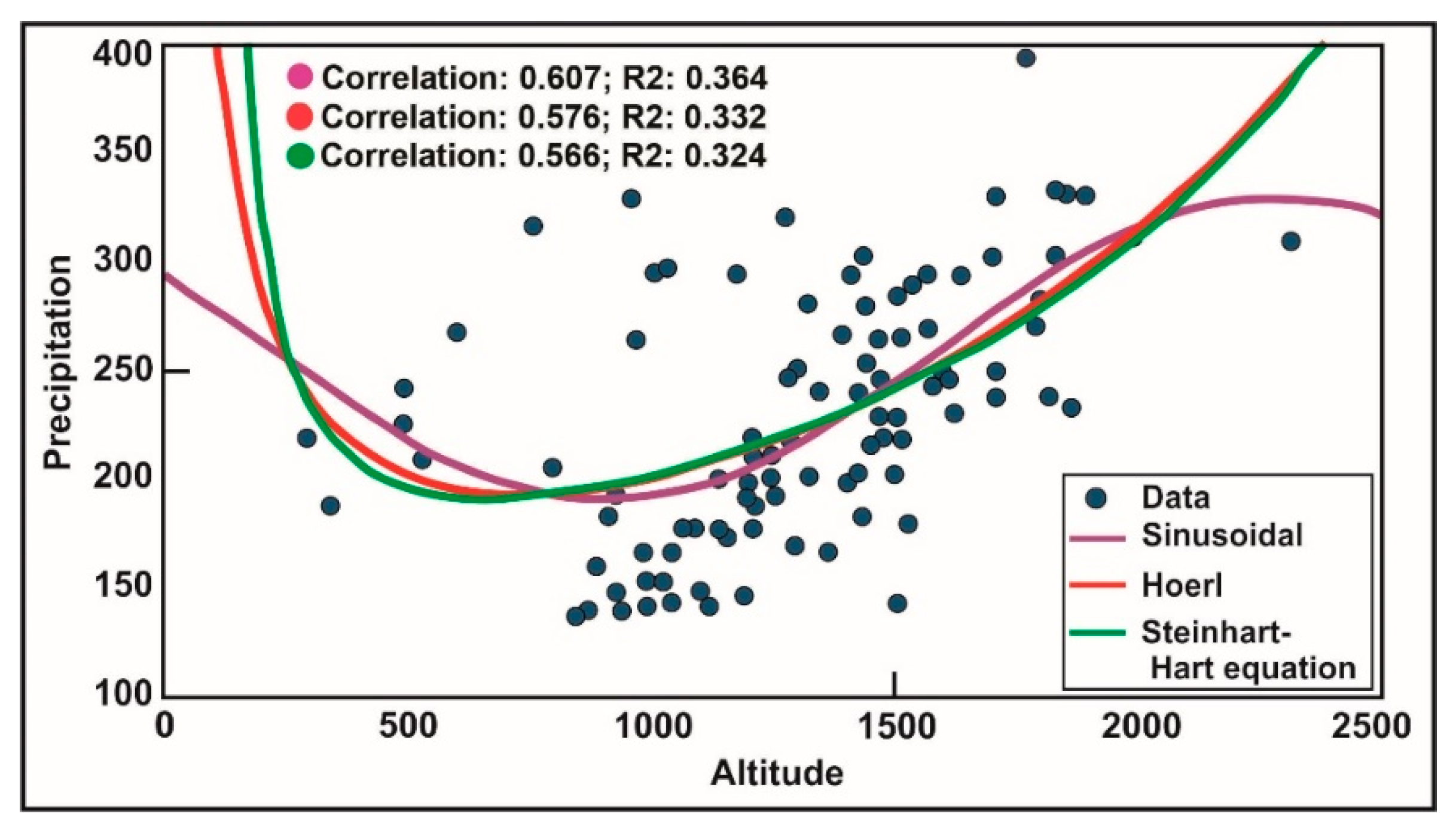
3.2.5. Non-Linear Regression Method
4. Discussion
5. Conclusions
Supplementary Materials
Author Contributions
Funding
Institutional Review Board Statement
Informed Consent Statement
Data Availability Statement
Acknowledgments
Conflicts of Interest
Appendix A
Semi-Variogram
Appendix B
Cross Semi-Variogram
References
- Greco, A.; De Luca, D.L.; Avolio, E. Heavy precipitation systems in Calabria Region (Southern Italy): High-resolution observed rainfall and large-scale atmospheric pattern analysis. Water 2020, 12, 1468. [Google Scholar] [CrossRef]
- Taesombat, W.; Sriwongsitanon, N. Areal rainfall estimation using spatial interpolation techniques. Sci. Asia 2009, 35, 268–275. [Google Scholar] [CrossRef]
- Jun, L. Development of Isohyet Map Using Inverse Distance Weighting and Ordinary Kriging Methods. Bachelor Thesis, Faculty of Civil Engineering and Earth Resources, University of Malaysia Pahang, Pahang, Malaysia, 2018. [Google Scholar]
- González-Álvarez, Á.; Viloria-Marimón, O.M.; Coronado-Hernández, Ó.E.; Vélez-Pereira, A.M.; Tesfagiorgis, K.; Coronado-Hernández, J.R. Isohyetal maps of daily maximum rainfall for different return periods for the Colombian Caribbean Region. Water 2019, 11, 358. [Google Scholar] [CrossRef]
- Ly, S.; Charles, C.; Degre, A. Geostatistical interpolation of daily rainfall at catchment scale: The use of several variogram models in the Ourthe and Ambleve catchments, Belgium. Hydrol. Earth Syst. Sci. 2011, 15, 2259–2274. [Google Scholar] [CrossRef]
- Matos, J.P.; Liechti, T.C.; Portela, M.M.; Schleiss, A.J. Pattern-oriented memory interpolation of sparse historical rainfall records. J. Hydrol. 2014, 510, 493–503. [Google Scholar] [CrossRef]
- Zhang, Y.; Vaze, J.; Chiew, F.H.; Teng, J.; Li, M. Predicting hydrological signatures in ungauged catchments using spatial interpolation, index model, and rainfall–runoff modelling. J. Hydrol. 2014, 517, 936–948. [Google Scholar] [CrossRef]
- Nikolopoulos, E.I.; Borga, M.; Creutin, J.D.; Marra, F. Estimation of debris flow triggering rainfall: Influence of rain gauge density and interpolation methods. Geomorphology 2015, 243, 40–50. [Google Scholar] [CrossRef]
- Plouffe, C.C.; Robertson, C.; Chandrapala, L. Comparing interpolation techniques for monthly rainfall mapping using multiple evaluation criteria and auxiliary data sources: A case study of Sri Lanka. Environ. Modell. Softw. 2015, 67, 57–71. [Google Scholar] [CrossRef]
- Zhang, T.; Xu, X.; Xu, S. Method of establishing an underwater digital elevation terrain based on kriging interpolation. Measurement 2015, 63, 287–298. [Google Scholar] [CrossRef]
- Bhunia, G.S.; Shit, P.K.; Maiti, R. Comparison of GIS-based interpolation methods for spatial distribution of soil organic carbon (SOC). J. Saudi Soc. Agric. Sci. 2016, 17, 114–126. [Google Scholar] [CrossRef]
- Mendez, M.; Calvo-Valverde, L. Assessing the performance of several rainfall interpolation methods as evaluated by a conceptual hydrological model. Procedia Eng. 2016, 154, 1050–1057. [Google Scholar] [CrossRef]
- Caruso, C.; Quarta, F. Interpolation methods comparison. Comput. Math. Appl. 1998, 35, 109–126. [Google Scholar] [CrossRef]
- Chen, T.; Ren, L.; Yuan, F.; Yang, X.; Jiang, S.; Tang, T.; Zhang, L. Comparison of spatial interpolation schemes for rainfall data and application in hydrological modeling. Water 2017, 9, 342. [Google Scholar] [CrossRef]
- İçağa, Y.; Emin, T.A.Ş. Comparative Analysis of Different Interpolation Methods in Modeling Spatial Distribution of Monthly Precipitation. Doğal Afetler ve Çevre Dergisi 2018, 4, 89–104. [Google Scholar] [CrossRef][Green Version]
- Huang, H.; Liang, Z.; Li, B.; Wang, D. A new spatial precipitation interpolation method based on the information diffusion principle. Stoch. Environ. Res. Risk Assess. 2019, 33, 765–777. [Google Scholar] [CrossRef]
- Liu, D.; Zhao, Q.; Fu, D.; Guo, S.; Liu, P.; Zeng, Y. Comparison of spatial interpolation methods for the estimation of precipitation patterns at different time scales to improve the accuracy of discharge simulations. Hydrol. Res. 2020, 51, 583–601. [Google Scholar] [CrossRef]
- Yang, X.; Xie, X.; Liu, D.L.; Ji, F.; Wang, L. Spatial Interpolation of Daily Rainfall Data for Local Climate Impact Assessment over Greater Sydney Region. Adv. Meteorol. 2015, 2015, 563629. [Google Scholar] [CrossRef]
- Zeinivand, H. Comparison of interpolation methods for precipitation fields using the physically based and spatially distributed model of river runoff on the example of the Gharesou basin, Iran. Russ. Meteorol. Hydrol. 2015, 40, 480–488. [Google Scholar] [CrossRef]
- Zhang, X.; Lu, X.; Wang, X. Comparison of Spatial Interpolation Methods Based on Rain Gauges for Annual Precipitation on the Tibetan Plateau. Pol. J. Environ. Stud. 2016, 25, 1339–1345. [Google Scholar] [CrossRef]
- Foehn, A.; Hernández, J.G.; Schaefli, B.; De Cesare, G. Spatial interpolation of precipitation from multiple rain gauge networks and weather radar data for operational applications in Alpine catchments. J. Hydrol. 2018, 563, 1092–1110. [Google Scholar] [CrossRef]
- Guo, B.; Zhang, J.; Meng, X.; Xu, T.; Song, Y. Long-term spatio-temporal precipitation variations in China with precipitation surface interpolated by ANUSPLIN. Sci. Rep. 2020, 10, 1–17. [Google Scholar] [CrossRef] [PubMed]
- Soleymani Moghadam, M.; Bani Assad, T. An analysis of the urban network of Khorasan Razavi province during the years 1986 to 2011. Q. J. Geogr. Urban Plan. Zagros Vis. 2017, 9, 45–67. (In Persian) [Google Scholar]
- Sakhdari, H.; Ziaei, S. Khorasan Razavi agricultural development priorities: Hierarchical Analysis (AHP) approach. J. Agric. Econ. Res. 2018, 1, 207–224. (In Persian) [Google Scholar]
- Araste, M.; Kaboli, H.; Yazdani, M. Assessing the impacts of meteorological drought on yield of rainfed wheat and barley (Case study: Khorasan Razavi province). Sci. J. Agric. Meteorol. 2017, 5, 15–25. [Google Scholar]
- Emadodin, I.; Reinsch, T.; Taube, F. Drought and desertification in Iran. Hydrology 2019, 6, 66. [Google Scholar] [CrossRef]
- Alijani, B.; Herman, J.R. Synoptic climatology of precipitation in Iran. Ann. Assoc. Am. Geogr. 1985, 75, 404–416. [Google Scholar] [CrossRef]
- Chang, K. Introduction to Geographic Information Systems, 3rd ed.; McGrawHill: New York, NY, USA, 2006. [Google Scholar]
- Aguilar, F.J.; Agüera, F.; Aguilar, M.A.; Carvajal, F. Effects of precipitation morphology, sampling density, and interpolation methods on grid DEM accuracy. Photogramm. Eng. Remote Sens. 2005, 71, 805–816. [Google Scholar] [CrossRef]
- Xie, Y.; Chen, T.B.; Lei, M.; Yang, J.; Guo, Q.J.; Song, B.; Zhou, X.Y. Spatial distribution of soil heavy metal pollution estimated by different interpolation methods: Accuracy and uncertainty analysis. Chemosphere 2011, 82, 468–476. [Google Scholar] [CrossRef] [PubMed]
- Bhattacharjee, S.; Mitra, P.; Ghosh, S.K. Spatial interpolation to predict missing attributes in GIS using semantic kriging. IEEE Trans. Geosci. Remote Sens. 2013, 52, 4771–4780. [Google Scholar] [CrossRef]
- Wood, C.; Miller, B. Comparing Simple and Ordinary Kriging Methods for 2015 Iowa Precipitation; Geological and Atmospheric Sciences; College of Liberal Arts and Sciences, Iowa State University: Ames, IA, USA, 2016. [Google Scholar]
- Lichtenstern, A. Kriging Methods in Spatial Statistics. Bachelor’s Thesis, Department of Mathematics, Technical University of Munich, Munich, Germany, 2013. [Google Scholar]
- İmamoğlu, M.Z.; Sertel, E. Analysis of different interpolation methods for soil moisture mapping using field measurements and remotely sensed data. Int. J. Environ. Geoinform. 2016, 3, 11–25. [Google Scholar] [CrossRef]
- Maris, F.; Kitikidou, K.; Angelidis, P.; Potouridis, S. Kriging interpolation method for estimation of continuous spatial distribution of precipitation in Cyprus. Curr. J. Appl. Sci. Technol. 2013, 1286–1300. [Google Scholar] [CrossRef]
- Qing, L.I.; Yu, Y.A.N.G. Cross-Modal Multimedia Information Retrieval. In Encyclopedia of Database Systems; Springer: Berlin/Heidelberg, Germany, 2009; pp. 528–532. [Google Scholar]
- Sun, Y.; Kang, S.; Li, F.; Zhang, L. Comparison of interpolation methods for depth to groundwater and its temporal and spatial variations in the Minqin oasis of northwest China. Environ. Model. Softw. 2009, 24, 1163–1170. [Google Scholar] [CrossRef]
- Gan, W.; Chen, X.; Cai, X.; Zhang, J.; Feng, L.; Xie, X. Spatial interpolation of precipitation considering geographic and topographic influences—A case study in the Poyang Lake Watershed, China. In Proceedings of the 2010 IEEE International Geoscience and Remote Sensing Symposium, Honolulu, HI, USA, 25–30 July 2010; pp. 3972–3975. [Google Scholar]
- Yang, G.; Zhang, J.; Yang, Y.; You, Z. Comparison of interpolation methods for typical meteorological factors based on GIS—A case study in Ji Tai basin, China. In Proceedings of the 19th International Conference on Geoinformatics, Shanghai, China, 24–26 June 2011; pp. 1–5. [Google Scholar]
- Wu, C.Y.; Mossa, J.; Mao, L.; Almulla, M. Comparison of different spatial interpolation methods for historical hydrographic data of the lowermost Mississippi River. Ann. GIS 2019, 25, 133–151. [Google Scholar] [CrossRef]
- Magnard, C.; Werner, C.; Wegmüller, U. GAMMA Technical Report: Interpolation and Resampling; Gamma Remote Sensing Research and Consulting AG: Bern, Switzerland, 2017. [Google Scholar]
- Goovaerts, P. Kriging and semivariogram deconvolution in the presence of irregular geographical units. Math. Geosci. 2017, 40, 101–128. [Google Scholar] [CrossRef]
- Mehrshahi, D.; Khosravi, Y. The assessment of Kriging interpolation methods and Linear Regression based on digital elevation model (DEM) in order to specify the spatial distribution of annual precipitation (Case study: Isfahan Province). J. Spatial Plan. 2010, 14, 233–249. [Google Scholar]
- Mahmoudvand, S.; Khodayari, H.; Tarnian, F. Mapping Bioclimatic Variables Using Geostatistical and Regression Techniques in Lorestan Province. JGSMA 2020, 1, 1–17. (In Persian) [Google Scholar]
- Dirks, K.N.; Hay, J.E.; Stow, C.D.; Harris, D. High-resolution studies of precipitation on Norfolk Island Part II: Interpolation of precipitation data. J. Hydrol. 1998, 208, 187–193. [Google Scholar] [CrossRef]
- Ahrens, B. Distance in spatial interpolation of daily rain gauge data. Hydrol. Earth Syst. Sci. 2006, 10, 197–208. [Google Scholar] [CrossRef]
- Keblouti, M.; Ouerdachi, L.; Boutaghane, H. Spatial interpolation of annual precipitation in Annaba-Algeria—Comparison and evaluation of methods. Energy Procedia 2012, 18, 468–475. [Google Scholar] [CrossRef]
- Martinez, C.A. Multivariate geostatistical analysis of evapotranspiration and precipitation in mountainous terrain. J. Hydrol. 1996, 174, 19–35. [Google Scholar] [CrossRef]
- Goovaerts, P. Geostatistical approaches for incorporating elevation into the spatial interpolation of rainfall. J. Hydrol. 2000, 228, 113–129. [Google Scholar] [CrossRef]
- Wang, X.; Lv, J.; Wei, C.; Xie, D. Modeling spatial pattern of precipitation with GIS and multivariate geostatistical methods in Chongqing tobacco planting region, China. In Proceedings of the International Conference on Computer and Computing Technologies in Agriculture, Nanchang, China, 22–25 October 2010; Springer: Berlin/Heidelberg, Germany, 2010; pp. 512–524. [Google Scholar]
- Hu, Y. Mapping Monthly Precipitation in Sweden by Using GIS; Göteborg University: Göteborg, Sweden, 2010. [Google Scholar]
- Di Piazza, A.; Lo Conti, F.; Noto, L.V.; Viola, F.; La Loggia, G. Comparative analysis of different techniques for spatial interpolation of precipitation data to create a serially complete monthly time series of precipitation for Sicily, Italy. Int. J. Appl. Earth Obs. 2011, 13, 396–408. [Google Scholar] [CrossRef]
- Bostan, P.A.; Heuvelink, G.B.M.; Akyurek, S.Z. Comparison of regression and kriging techniques for mapping the average annual precipitation of Turkey. Int. J. Appl. Earth Obs. 2012, 19, 115–126. [Google Scholar] [CrossRef]
- Hao, W.; Chang, X. Comparison of spatial interpolation methods for precipitation in Ningxia, China. Int. J. Sci. Res. 2013, 2, 181–184. [Google Scholar]
- Abo-Monasar, A.; Al-Zahrani, M.A. Estimation of rainfall distribution for the southwestern region of Saudi Arabia. Hydrol. Sci. J. 2014, 59, 420–431. [Google Scholar] [CrossRef]
- Isaaks, E.H.; Srivastava, R.M. An Introduction to Applied Geostatistics; Oxford University Press: New York, NY, USA, 1989. [Google Scholar]


| Station | Longitude | Latitude | Altitude (m a.s.l.) | Station | Longitude | Latitude | Altitude (m a.s.l.) | Station | Longitude | Latitude | Altitude (m a.s.l.) |
|---|---|---|---|---|---|---|---|---|---|---|---|
| Emamzadeh-Mayamey | 76°88′68″ | 40°35′25.1″ | 1039 | Dolatabad Khoramdareh | 69°31′77″ | 40°39′80.0″ | 1575 | Khatiteh | 51°74′98″ | 40°46′84.0″ | 1435 |
| Balghoor | 71°36′48″ | 40°67′52.4″ | 1941 | Hey Hey Ghoochan | 63°58′99″ | 41°08′34.3″ | 1344 | Marosk | 63°86′67″ | 40°43′51.6″ | 1525 |
| Zoshk | 72°69′04″ | 40°86′07.6″ | 1832 | Sanobar | 69°37′55″ | 39°21′18.2″ | 1707 | Hendelabad | 72°58′93″ | 39°89′92.5″ | 1206 |
| Bakvol | 69°52′22″ | 39°29′72.8″ | 1849 | Namegh | 65°96′98″ | 39°20′54.7″ | 1815 | Hosseinabad | 62°45′86″ | 39°88′70.7″ | 1072 |
| Ghonchi | 70°15′02″ | 39°32′19.3″ | 1892 | Nari | 73°96′95″ | 39°42′62.5″ | 1861 | Karat | 75°41′55″ | 38°75′63.2″ | 1084 |
| Chakaneh Olya | 72°70′59″ | 40°77′15.7″ | 1704 | Kalateh Rahman | 74°69′26″ | 39°62′05.3″ | 1619 | Ghand e Jovein | 53°61′66″ | 40°54′89.2″ | 1140 |
| Darband Kalat | 74°95′86′ | 40°78′20.3″ | 960 | Sharifabad-Kashafrood | 70°85′08″ | 40°21′00.1″ | 1467 | Rashtkhar | 63°18′58″ | 38°52′25.2″ | 1155 |
| Dizbad | 70°51′49″ | 39°97′75.9″ | 1988 | Farhadgerd-Fariman | 74°84′55″ | 39°40′39.7″ | 1503 | Sangerd | 60°30′34″ | 39°61′80.5″ | 1291 |
| Archangan | 74°26′34″ | 40°98′00.7″ | 757 | Chahchaheh | 73°11′33″ | 40°73′49.8″ | 486 | Kalateh | 71°40′70″ | 40°01′73.9″ | 983 |
| Jang | 67°64′01″ | 40°74′98.4″ | 2313 | Dargaz | 64°53′23″ | 41°64′51.6″ | 494 | Sahlabad | 73°06′76″ | 39°05′49.4″ | 1360 |
| Mareshk | 74°06′95″ | 40°56′09.3″ | 1830 | Hatamghaleh | 72°14′81″ | 41°12′76.6″ | 493 | Irajabad | 60°61′76″ | 39°03′17.0″ | 1041 |
| Yengjeh abshar | 61°27′00″ | 40°76′67.8″ | 1703 | Ghand Torbat | 70°14′68″ | 39°13′15.1″ | 1474 | Ghand Torbatjam | 75°75′41″ | 39°53′87.6″ | 888 |
| Mohammad Taghi Beyg | 62°84′49″ | 41°61′05.4″ | 1009 | Ghare Shisheh | 76′16″40° | 39°37′56.5″ | 1512 | Edareh Mashhad | 69°70′23″ | 40°23′74.2″ | 1018 |
| Talghor | 67°63′94″ | 40°40′11.4″ | 1563 | Beyroot | 60°40′18″ | 39°51′53.0″ | 1452 | Sharifabad | 55°94′24″ | 39°10′36.0″ | 1100 |
| Ferizi | 67°40′19″ | 40°51′60.6″ | 1631 | Andarokh | 70°97′98″ | 40°30′68.6″ | 1207 | Janatabad | 71°01′54″ | 38°46′69.3″ | 925 |
| Eishabad | 66°43′19″ | 40°18′99.4″ | 1406 | Sad Torogh | 63°16′77″ | 40°78′32.1″ | 1242 | Chenaran | 74°30′31″ | 39°98′62.8″ | 1186 |
| Saghbeig | 62°67′89″ | 40°64′65.2″ | 1532 | Karkhaneh Ghand | 64°34′74″ | 40°17′69.6″ | 1207 | Kashmar | 63°26′35″ | 38°99′53.5″ | 1503 |
| Taghoon | 65°09′47″ | 40°32′14.9″ | 1503 | Gharehtikan | 72°49′66″ | 41°15′04.3″ | 527 | Sabzevar | 56°15′69″ | 40°08′14.9″ | 988 |
| Kariz No | 83°63′25″ | 38°93′23.1″ | 1798 | Dahneh Shoor | 59°61′67″ | 40°48′15.0″ | 1243 | Gonabad | 65°49′15″ | 38°01′27.5″ | 1117 |
| Ardak | 72°95′87″ | 40°06′13.2″ | 1320 | Kariz Kashmar | 61°79′71″ | 39°25′09.9″ | 1420 | Darooneh | 53°71′94″ | 38°92′74.1″ | 870 |
| Kapkan | 66°93′47″ | 41°24′35.3″ | 1437 | Talkhbakhsh | 66°83′64″ | 39°54′93.2″ | 1496 | Mazinan | 48°33′62″ | 40°19′47.1″ | 848 |
| Moghan | 69°05′38″ | 40°57′48.2″ | 1788 | Sheikh Abolghasem | 69°99′75″ | 39°01′17.0″ | 1320 | Bezangan | 81°94′49″ | 40°22′02.4″ | 1027 |
| Goosh Bala | 73°18′37″ | 40°30′50.6″ | 1569 | Kartian | 71°60′22″ | 40°20′75.1″ | 1240 | Fadak | 75°86′40″ | 38°50′12.3″ | 991 |
| Agh Darband | 75°24′70″ | 40°15′90.5″ | 602 | Roohabad | 66°71′86″ | 39°92′84.4″ | 1138 | Shahrno Bakharz | 80°31′88″ | 38°76′84.0″ | 1282 |
| Tabarokabad | 65°27′15″ | 41°17′00.7″ | 1510 | Ghadirabad | 71°05′44″ | 40°78′18.3″ | 1195 | Sangar Sarakhs | 87°71′56″ | 40°14′52.2″ | 343 |
| Al | 72°89′19″ | 40°66′63.3″ | 1464 | Zarandeh | 63°44′80″ | 40°37′28.0″ | 1403 | Hesar Dargaz | 71°17′68″ | 41°46′14.6″ | 289 |
| Gardaneh Kalat | 63°56′16″ | 37°80″69.7″ | 966 | Mozdooran | 73°80′58″ | 40°51′80.8″ | 927 | Sad Kardeh | 73°94′44″ | 40°56″35.5′ | 1279 |
| Golmakan | 67°69′40″ | 40°39′72.8″ | 1440 | Dereakht Toot | 71°96′53″ | 40°71′55.5″ | 1254 | Abghad Ferizi | 67°59′48″ | 40°40′22.3″ | 1390 |
| Sarasiab | 73°10′51″ | 40°21′77.9″ | 1296 | Malekabad | 71°79′93″ | 38°90′87.3″ | 1195 | Zirban Golestan | 70°70′16″ | 40°21′26.9″ | 1434 |
| Cheharbagh | 65°41′56″ | 40°46′18.4″ | 1599 | Emamzadeh-Radkan | 74°02′51″ | 39°35′00.5″ | 1214 | Fariman | 75°74′80″ | 39°53′90.3″ | 1419 |
| Taroosk | 70°13′99″ | 39°27′39.7″ | 1704 | Olang e Asadi | 72°60′73″ | 40°05′93.0″ | 912 | Timnak Sofla | 82°65′63″ | 39°32′37.0″ | 1176 |
| Fadiheh | 67°46′92″ | 39°16′82.4″ | 1611 | Bagh Sangan | 78°82′12″ | 38°29′78.5″ | 937 | Deh Menj | 80°21′48″ | 38°79′86.7″ | 1273 |
| Dahaneh Akhlamad | 65°16′63″ | 40°78′63.2″ | 1467 |
| Min | Max | Mean | Std.Dev | Skewness | Kurtosis | CV |
|---|---|---|---|---|---|---|
| 137 | 400 | 229.77 | 58.081 | 0.131 | 2.44 | 25.669 |
| Method | RMSE | MAE | |
|---|---|---|---|
| Completely Regularized Spline | 52.57 | 1.120 | 0.177 |
| Spline with Tension | 52.46 | 1.116 | 0.179 |
| Multiquadric | 61.21 | 1.515 | 0.098 |
| Inverse Multiquadric | 53.39 | 1.060 | 0.147 |
| Thin Plate Spline | 270.87 | 2.490 | 0.048 |
| Method | Semi-Variogram Theoretical Model (Appendix A) | RMSE | MAE | |
|---|---|---|---|---|
| Ordinary (OK) | Circular | 51.33 | 1.128 | 0.211 |
| Simple (SK) | Hole Effect | 50.90 | 1.145 | 0.224 |
| Universal (UK) | Exponential | 51.33 | 1.128 | 0.211 |
| Method | Cross Semi-Variogram Theoretical Model | RMSE | MAE | |
|---|---|---|---|---|
| OCoK | K-Bessel | 42.18 | 1.108 | 0.468 |
| SCoK | K-Bessel | 45.45 | 0.777 | 0.377 |
| UCoK | Exponential | 42.18 | 1.108 | 0.468 |
| Method | RMSE | MAE | R2 |
|---|---|---|---|
| Sinusoidal | 56.73 | 1.477 | 0.119 |
| Hoerl | 56.37 | 0.707 | 0.111 |
| Steinhart-Hart Equation | 55.63 | 0.699 | 0.110 |
| Method (in the Case of Several Sub-Methods, the Best-Performing One Was Selected) | RMSE | MAE | |
|---|---|---|---|
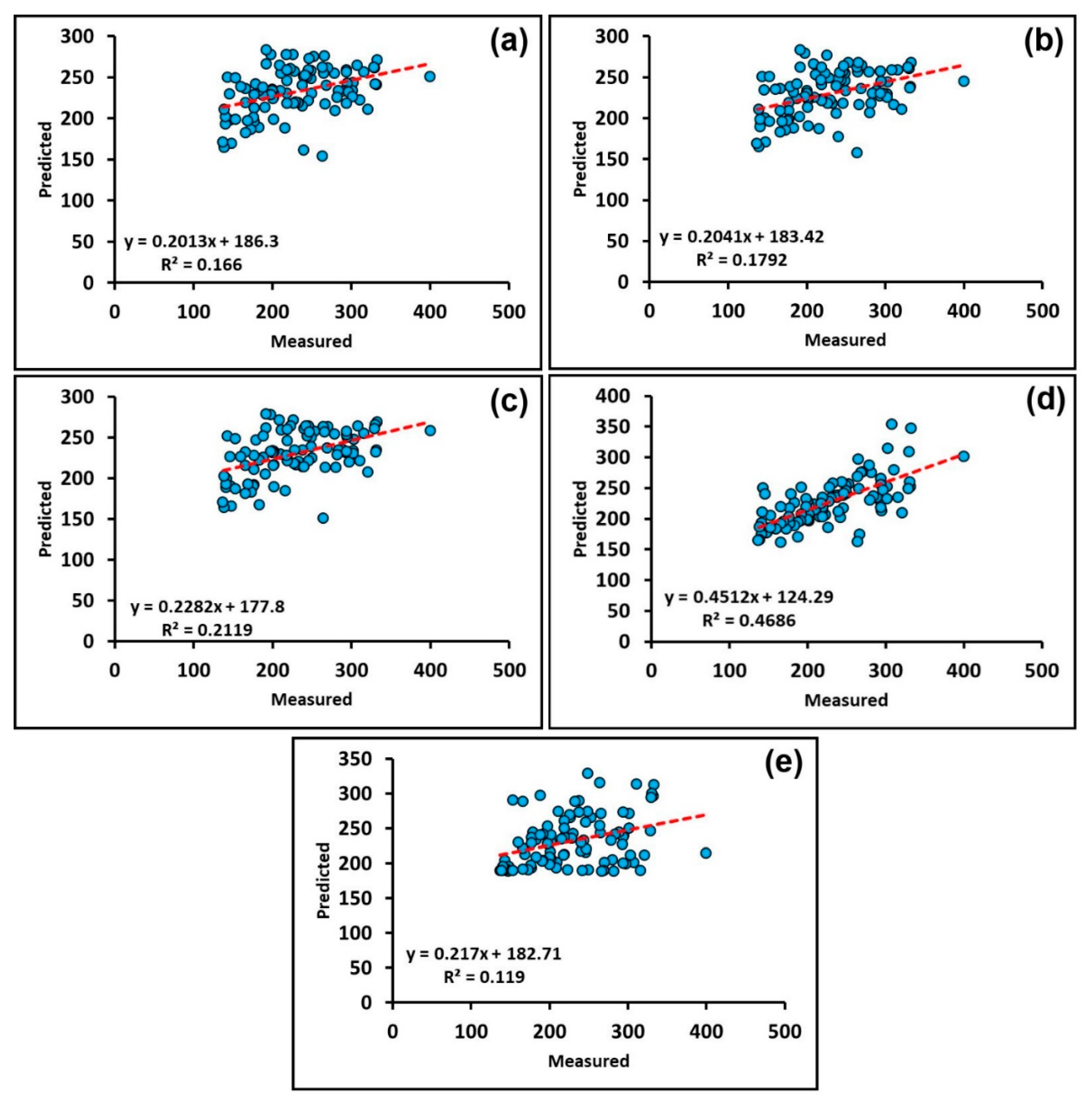
| IDW | 53.07 | 1.108 | 0.166 |
| RBF (Spline with Tension) | 52.46 | 1.116 | 0.179 |
| Kriging (Simple Kriging) | 50.90 | 1.145 | 0.220 |
| Co-Kriging (Ordinary and Universal Co-Kriging) | 42.18 | 1.108 | 0.469 |
| Non-linear regression (Sinusoidal) | 56.73 | 1.477 | 0.119 |
Publisher’s Note: MDPI stays neutral with regard to jurisdictional claims in published maps and institutional affiliations. |
© 2021 by the authors. Licensee MDPI, Basel, Switzerland. This article is an open access article distributed under the terms and conditions of the Creative Commons Attribution (CC BY) license (https://creativecommons.org/licenses/by/4.0/).
Share and Cite
Aalijahan, M.; Khosravichenar, A. A Multimethod Analysis for Average Annual Precipitation Mapping in the Khorasan Razavi Province (Northeastern Iran). Atmosphere 2021, 12, 592. https://doi.org/10.3390/atmos12050592
Aalijahan M, Khosravichenar A. A Multimethod Analysis for Average Annual Precipitation Mapping in the Khorasan Razavi Province (Northeastern Iran). Atmosphere. 2021; 12(5):592. https://doi.org/10.3390/atmos12050592
Chicago/Turabian StyleAalijahan, Mehdi, and Azra Khosravichenar. 2021. "A Multimethod Analysis for Average Annual Precipitation Mapping in the Khorasan Razavi Province (Northeastern Iran)" Atmosphere 12, no. 5: 592. https://doi.org/10.3390/atmos12050592
APA StyleAalijahan, M., & Khosravichenar, A. (2021). A Multimethod Analysis for Average Annual Precipitation Mapping in the Khorasan Razavi Province (Northeastern Iran). Atmosphere, 12(5), 592. https://doi.org/10.3390/atmos12050592