Measurements of NO_x and Development of Land Use Regression Models in an East-African City

Abstract

Air pollution causes premature mortality and morbidity globally, but these adverse health effects occur over proportionately in low- and middle-income countries. Lack of both air pollution data and knowledge of its spatial distribution in African countries have been suggested to lead to an underestimation of health effects from air pollution. This study aims to measure nitrogen oxides (NO_x), as well as nitrogen dioxide (NO₂), to develop Land Use Regression (LUR) models in the city of Adama, Ethiopia. NO_x and NO₂ was measured at over 40 sites during six days in both the wet and dry seasons. Throughout the city, measured mean levels of NO_x and NO₂ were 29.0 µg/m³ and 13.1 µg/m³, respectively. The developed LUR models explained 68% of the NO_x variances and 75% of the NO₂. Both models included similar geographical predictor variables (related to roads, industries, and transportation administration areas) as those included in prior LUR models. The models were validated by using leave-one-out cross-validation and tested for spatial autocorrelation and multicollinearity. The performance of the models was good, and they are feasible to use to predict variance in annual average NO_x and NO₂ concentrations. The models developed will be used in future epidemiological and health impact assessment studies. Such studies may potentially support mitigation action and improve public health.

1. Introduction

Epidemiological studies have shown that ambient air pollution is the single-largest environmental health risk worldwide [1]. Globally, outdoor air pollution exposure is responsible for 3.3 million premature deaths [2], with some estimates putting this number as high as 8.9 million deaths per year [3].

Nitrogen oxides (NO_x) and nitrogen dioxide (NO₂), in particular, are anthropogenically generated components of air pollution [4]. Even though NO_x is primarily emitted in the form of NO during combustion, which is then oxidized to NO₂, NO₂ has often been used as marker of air pollution exposure in epidemiological studies to determine the adverse health effects such as birth outcomes in epidemiological studies [5,6]. For example, exposure to NO_x is associated with cause-specific mortality and myocardial infraction [7], as well as adverse birth outcomes, including impaired childhood lung function [8] spontaneous abortion [9], preterm birth [10], low birth weight [11], fetal growth restriction [12], gestational hypertension, and preeclampsia [13,14]. The economic cost of these air pollution-derived health effects is also expected to decrease the global domestic product (GDP) by one percent by 2060 [15].

Establishing urban air pollution monitoring systems and setting air quality standards are crucial in alleviating the public health challenges related to air pollution. Unfortunately, air pollution monitoring is vastly lacking in Africa [16]. There are only a few epidemiological studies on the links between ambient air pollution and long- and short-term health effects in African settings. The lack of long-term ambient air pollution monitoring has been emphasized as a reason [17]. Few studies in Africa reported urban air pollution variability and explored the link between ambient air pollution and respiratory morbidity [18,19]. Without data on the extent of air pollution exposure, health impacts remain underestimated or even unknown; this prevents the implementation of key public health strategies, especially those needed to protect vulnerable populations such as pregnant women and children [20].

In East Africa, in particular, common challenges to air pollution mitigation include growing vehicle fleets, a lack of alternative cleaner energy sources for industries, rapid urbanization, poor urban infrastructure, uncontrolled open burning, limited air quality data, weak enforcement of policies, and limited technical capacity and financial resources [21,22]. Typical sources of ambient air pollution are road traffic, industries, domestic fires for cooking or heating, and waste burning [23]. For instance, the prevalence of old, polluting vehicles coupled with poor maintenance practices has led to vehicle emission being the region’s main source of air pollution [24,25]. Household waste burning is also a major contributor to ambient air pollution [26]. More effort is urgently needed from African governments to develop and enforce air quality standards; however, this cannot be achieved without access to reliable air pollution and health data [25].

Air pollution measurements are needed for the utilization of Land Use Regression (LUR), which has, consequently been lacking in African settings [27]. The LUR model is a tool commonly used in epidemiological studies to assess ambient air pollution exposure, especially at locations with limited air pollution data [28]. This is accomplished by using measured pollution values as a response variable with local geographical predictor variables, which are potential proxies for emission sources, such as land use, population, household density, or traffic intensity [28,29]. LUR models have been widely applied in European [28,30] and North American [31,32] cities. The European Study of Cohort for Air Pollution Effects (ESCAPE) is a large-scale, EU-multicenter study encompassing several cities that has established comprehensive, well-designed LUR protocols [28]. Its methodology has even been applied in some parts of Asia [33]. To the best of our knowledge, only a few applications of the LUR model have been performed within the African continent to estimate NO_x or NO₂, as well as to assess the association between long-term ambient air pollution and health effects [18,19,34].

This study aims to generate reliable evidence on the ambient air pollution levels through measurements and use these to develop LUR models to estimate the NO_x and NO₂ exposure in Adama, Ethiopia. Over 13,000 premature deaths are attributed to ambient air pollution exposure annually in Ethiopia, which is the highest among East African countries [35]. The LUR exposure estimate will be used in future projects to further assess the health impacts of air pollution. As an example, it will be used to investigate the association between maternal exposure during pregnancy and the subsequent health outcomes of neonates in the Adama mother and child health cohort (ClinicalTrials.gov Identifier NCT03305991).

2. Materials and Methods

2.1. Study Site

Spanning 200 square kilometers, Adama is the fourth largest city in Ethiopia, with an estimated 214,000 inhabitants [36]. It is located 99 km southeast of Addis Ababa in the East African Rift Valley area (see Figure 1). The weather is mostly dry throughout the year, with a mean annual rainfall of 890 mm and mean annual temperature of 21.6 °C, with highest precipitation in June, July, and August [37]. Adama is located along the Pan-African Highway, connecting Djibouti with Addis Ababa. There is also a large bus station in the center of the city connecting the eastern and southeastern parts of the country.

Adama city has industrial and investment centers, clustered mainly in its western and eastern outskirts. A total of 144 large- and small-scale industrial operations, including paper printing, cement manufacturing, brick manufacturing, tomato-canning plants, cottage industries, textiles, food, and beverage factories, as well as metal, plastic, and wood engineering facilities, are located in the southwest [38]. The Adama public transportation service is operated by many small vehicles like the Bajaj (a compact, three wheeled car), which accounts for 70% of the total vehicle fleet, and a few public buses [38]. In 2015, the daily traffic volume at four main intersections in Adama was between 16,000 and 32,000 vehicles [39]. According to the Adama municipality, the total road length of the asphalt is 95 km, with gravel roads stretching 56 km, cobblestone 170 km, red ash 36 km, and earth roads 740 km [38].

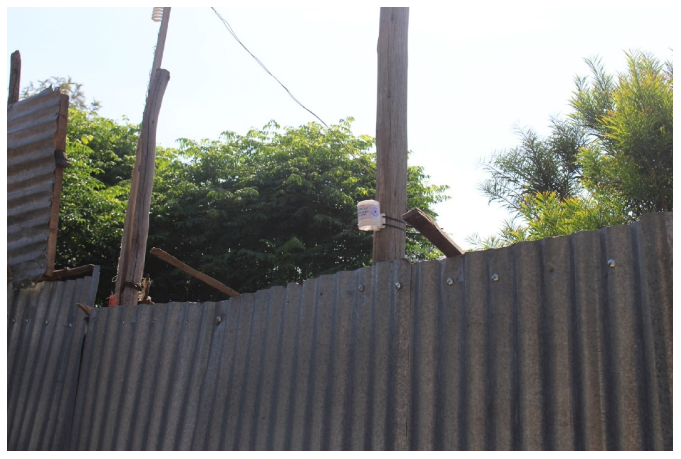
2.2. NO_x and NO₂ Sampling

Measurement sites were selected in accordance with the ESCAPE protocol to capture the anticipated variability of air pollution [40]. In this study, 41 individual sites were investigated in August 2018 and 42 sites in February 2019. One site from the August 2018 campaign was lost due to an analytical error for NO₂, but the values for NO_x remained viable. Between the two campaigns, 39 sites had measurements from both periods for NO_x and 38 sites for NO₂. One site included in the August 2018 campaign could not be used in the February 2019 campaign, as the landowner declined participation. Additionally, we added two sites to the February 2019 campaign that were unavailable in the August 2018 campaign. In total, 43 sites were included in the development of the LUR models, irrespective of whether they were utilized in one or both measurement campaigns. In the case of two measurements, we included the mean of both.

All field samplings were performed from 9–14 August (5 days) 2018 (wet season) and from 18–23 February (5 days) 2019 (dry season). The sampling sites were classified into three types: traffic (10 sites), urban background (27 sites), and regional background (6 sites). A traffic site is identified as an area where the air pollution level is mainly influenced by vehicle emissions from road traffic (in this study, the sites were located within 100 m from a motorway or primary or secondary road). An urban background site, however, is an urban area that is not heavily influenced by nearby traffic or industrial air pollution sources (sites in the city not located within 100 m from a motorway or primary or secondary road). Finally, a regional background site is defined as an area in which air pollution is not dominantly produced by any nearby sources but, rather, transported into the area by wind (sites located in the outskirts of the city not located close to a large industrial source or road construction site). This classification and distribution allowed us to choose the measurement sites representative for the air pollution levels throughout the city and its outskirts. Each measurement site’s location was geocoded and the altitude measured using a GARMIN GPSMAP64 (Garmin, Olathe, KS, USA) during each site visit.

According to the ESCAPE protocol [40], Ogawa badge passive samplers (Ogawa & Company, Pompano Beach, FL, USA) were used to sample NO₂ and NO_x. The Ogawa badge contains separate filters onto which NO_x and NO₂ are absorbed with high efficiency. In short, the Ogawa badge has a cylindrical body with two ends, which enables the simultaneous monitoring of NO₂ and NO_x. Each end holds a cellulose collection filter, one coated with triethanoleamine for sampling NO₂ and the other coated with triethanoleamine plus an oxidizing agent for sampling NO_x [41,42]. The badges were deployed at a height of 1.9–3.8 m under an opaque shelter for protection against rain (see Figure 2). Care was taken so that air could circulate freely around the unit. After sampling was completed, the badges were collected, stored in a cold box, and transported to Sweden together with four blanks. The samplers were delivered within 72 h to the lab.

All badges were analyzed at the Division of Occupational and Environmental Medicine, Umeå University, Umeå, Sweden. The analysis method was described in detail by Hagenbjork-Gustafsson et al. [41]. Briefly, each filter is desorbed in ultra-pure water; after, the filtered extract is injected into an ion chromatography system and analyzed for nitrite. The nitrite concentrations in the field blanks were subtracted from the concentrations in the samples. The obtained nitrite concentration was then used in an adapted version of Fick’s law [41] to calculate the NO₂ and NO_x concentrations.

2.3. Comparison to Active Measurments

In addition to the measurements taken with passive samplers, we were granted access to time-resolved NO₂ and NO_x data collected with a Thermo Scientific NO-NO₂-NO_x analyzer (model 42i) at the Ethiopian Meteorological Institute site in Adama.

One hundred and ninety-seven Microsoft^® Excel^® 2016 (Microsoft, Redmond, WA, USA) files containing minute-by-minute measurements of NO₂ and NO_x concentrations from the beginning of January 2017 through December 2018, as well as the month of January 2019, were accessed. First, duplicate files and those with cells expressing “NoData” were removed. Files corresponding to a 7-month period (August 2017–March 2018) were missing data on NO₂ and NO_x completely, and the vast majority of measurements throughout August 2018–January 2019 were missing. Moreover, a significant number of hours and days were comprised of very few data points (Figure S1).

When the data for a particular hour or day began with 0′s or negative values, those values were excluded for the calculations of hourly and daily averages. However, these 0′s and negative values also arose sporadically and could hence not be easily omitted from the averaging process. This combined with a lack of data for some hours, and days, even, resulted in a number of final NO₂ and NO_x averages being negative in value, averages all of which were not included in further evaluations.

Further, the quality of this data is uncertain, as there is no avilable information regarding calibaration of the instrument.

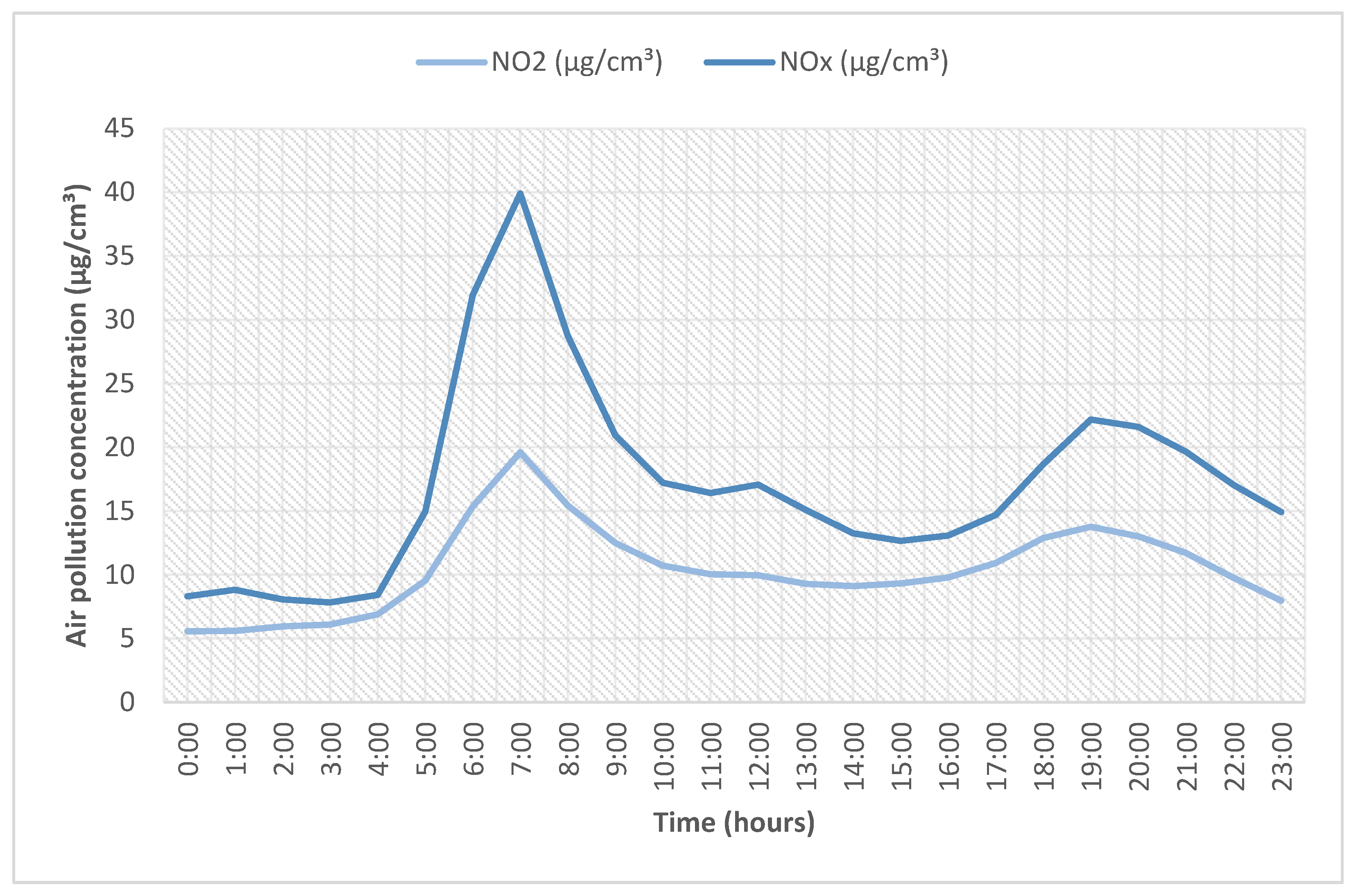
2.3.1. Diurnal Trends

As described above, the original measurement data, recorded minute-by-minute, was aggregated into hourly averages. This was later used to investigate diurnal trends of NO₂ and NO_x using Microsoft^® Excel^® 2016 (Microsoft, Redmond, WA, USA).

Only 18 days throughout this time period had complete data, i.e., included measurements for each of the 60 min for each of the 24 h in the day. From these, days falling on the weekend (n = 5) were excluded due to the expected differences in the traffic patterns. The NO₂ and NO_x concentrations from the remaining days (n = 13) were then averaged and graphed.

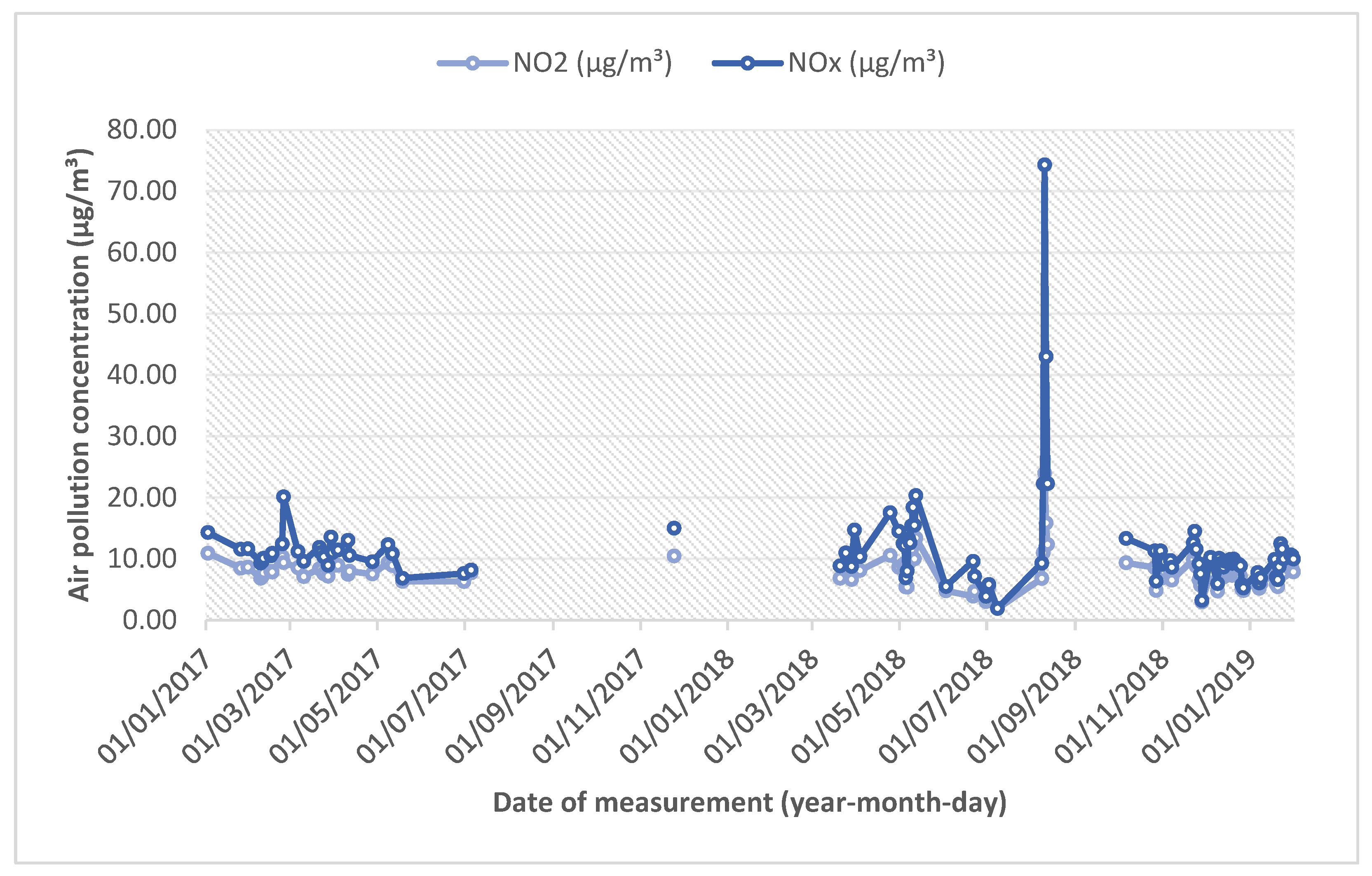
2.3.2. Yearly Concentrations

Original data from the time-resolved measurement instrument were also aggregated into daily averages, which were used to graph the annual trends of NO₂ and NO_x concentrations from January 2017 to January 2019. Further, the annual averages for both pollutants were calculated for the years 2017 and 2018, excluding measurements for the month of January 2019. Instead of using only days with complete data, as described above for the diurnal trends, here, all hours with ≥30 min of the measurements were included (1592 values out of 1702). Similarly, all days with ≥5 h of the measurements (the equivalent of 1140 min or more) were included, which totalled 103 out of 142 days.

2.4. Geographic Predictor Variables

A total of 59 geographical predictor variables were collected. For a full list of potential variables, see

Table 1. All the available geographic predictor variables, their expected direction of effects, and their descriptions.

Variables	Measurement Unit	Expected Direction of Effects
Less than 100 m to motor, primary, or secondary road	m	+
Inside the city center	yes/no	+
Measured altitude in meters above sea level	m	-
Road distance in meters within a 50, 100, 300 or 500 m radius	m	+
Primary road 1 distance in meters within a 50, 100, 300 or 500 m radius	m	+
Motorway in meters within a 500 m radius	m	+
Secondary road 2 distance within a 50, 100, 300 or 500 m radius	m	+
Tertiary road 3 distance within a 50, 100, 300 or 500 m radius	m	+
Residential road 4 distance within a 50, 100, 300 or 500 m radius	m	+
Service road 5 distance within a 50, 100, 300 or 500 m radius	m	+
Other road 6 in meters within a 50, 100, 300 or 500 m radius	m	+
Area of residential use within 100, 300, 1000 or 3000 m radius	m2	+
Area of industrial use within 100, 300, 1000 or 3000 m radius	m2	+
Area of transportation administration 7 use within 100, 300, 1000 or 3000 m radius	m2	+
Area of informal settlement within 100, 300, 1000 or 3000 m radius	m2	+
Distance to nearest primary road	m	-
Distance to nearest motorway	m	-
Distance to nearest secondary road	m	-
Distance to nearest tertiary road	m	-
Distance to nearest residential road	m	-
Distance to nearest service road	m	-
Distance to nearest other road	m	+
Distance to nearest road	m	-
Distance to nearest waterbody or creek/river	m	-
Distance to nearest industry	m	-
Distance to nearest transportation administration area	m	-
Primary road between 100 m and 300 m and 100 m and 500 m, respectively (only NOx)	m	+
Primary road between 300 m and 500 m (only NO2)	m	+
Road between 50 m and 100 m, 50 and 300 m, and 50 m and 500 m, respectively (only NOx)	m	+
Residential road between 100 and 300 m and 100 m and 500 m respectively (only NOx)	m	+
Residential area between 1000 m and 3000 m(both NO2 and NOx)	m	+

¹ The next most important roads in a country’s system (often link larger towns.). ² The next most important roads in a country’s system (often link towns.). ³ The next most important roads in a country’s system (often link smaller towns and villages). ⁴ Roads that serve as an access to housing, without function of connecting settlements. ⁵ Access roads to or within an industrial estate, camp site, business park, car park, alleys, etc. ⁶ Rural roads. ⁷ Bus stations and large parking lots.

. In addition to these, 2 outer ring buffer variables were added for NO₂ and 8 for NO_x [40]. A full description of the outer ring buffers can be found in the ESCAPE protocols [40]. These variables were univariately regressed against NO₂ and NO_x concentration at measurement sites. Previously published studies have demonstrated that the road variables, population density, land use, and elevation were significant predictor variables for the NO_x and NO₂ concentrations [28]. We defined the expected direction of the geographical predictor variables prior to the statistical analysis.

2.4.1. Land Use

The Adama city urban land development and management office masterplan from 2019 [43] was used to generate land use data. Four classes of land, including industrial areas, residential areas, water, and transportation facilities (see Figure 1), were identified as significant in relation to the NO_x and NO₂ emissions and were deemed manageable to adjust to the land use. This masterplan also contained areas with future land use plans. To replicate the conditions when our measurement campaigns were conducted, the areas mapped with future land use were manually adjusted using satellite images covering different parts of the city between 2016 and 2018. These included Worldview 2 (resolution 0.5 m) and Worldview 4 (resolution 0.31 m) [44], which were retrieved via World imagery in ArcMap. Corrections to the four land use classes, therefore, were mainly implemented in the outskirts of the city where the masterplan and the satellite images did not correspond. In addition to the land use information obtained from the masterplan, data on the informal settlement areas was collected and geocoded. For all land use variables, the total area covered in m² was calculated for 100-, 300-, 1000-, and 3000-m buffers around the measurement stations and added to the final model.

Industrial Areas

Industrial areas were considered potential sources of NO₂ and NO_x emissions within the study area. Since the masterplan´s data did not contain information about the type of industry, all industrial areas were assumed to contribute with equal emissions relative to their area. The average distance from a measurement site to the closest industrial area was 490 m, ranging from 35 to 1487 m.

Residential Areas

Residential areas describe places in Adama where human activity, such as waste burning and cooking, is likely to contribute to elevated levels of NO_x and NO₂. In the Adama city masterplan, different types of residential areas were included: housing, mixed residences (those intertwined with commercial land use), and residences. Since these three classes were not distinguishable in the satellite images, they were combined into one residential class for this study. Again, adjustments were made mainly along the outskirts of Adama, as new residential zones were being planned for these areas.

Water Bodies

The water bodies included in this study are seasonal pathways where water flows during the rainy season. During the dry season, however, these areas are used for solid waste burning and dumping. Waste burning can also occur in close vicinity to these areas during the rainy season. Data on water bodies were obtained from the masterplan and needed no adjustment in relation to the satellite images.

Transport Administration Areas

This class contains bus stations and major parking lots, which are most likely associated with higher NO_x and NO₂ levels due to traffic intensity. A total of 16 transport administration areas were included in our study, which were derived from the masterplan.

Informal Settlements

A high population density, old houses, and frequent small-scale waste burning are features associated with informal settlements that could contribute to higher levels of NO₂ and NO_x. This data was collected in the second half of 2019 by a local student with prior experience of collecting data with a GPS.

2.4.2. Road Traffic

Previous studies have often found traffic density and the road network distribution to be relevant variables to predict the NO_x and NO₂ levels [45]. The geographical distribution of Adama’s road network was accessed from OpenStreetMap [46] using a QGIS (QGIS Development Team (2020). QGIS Geographic Information System. Open Source Geospatial Foundation Project. http://qgis.osgeo.org (accessed on 15 April 2021)) plugin for the desktop geographic information systems (GIS) application QGIS and included information about the type of road, which was used as a proxy for the traffic intensity. A total of 16 different classes of roads were available. These were further categorized into seven classes, including Motorway, Primary, Secondary, Tertiary, Residential, Service, and Other roads. This reclassification process is described in detail in a recently published paper [47].

The GIS analysis was performed in ArcGIS version 10.5.1 (Redlands, CA, USA). All available geographic predictor variables are shown in Table 1.

2.5. Land Use Regression Modeling

The development of the LUR models followed the ESCAPE protocol [40]. A total of 59 predictor variables were univariately tested, followed by a manual forward selection procedure for the multivariate model. Statistically significant variables during the univariate testing were added to the multivariate model. A model that aimed to maximize the percentage of explained variability (R²) and minimize the error (RMSE—Root Mean Square Error) was selected. The variables with highest R² were added first, followed by the second, and so on. Only variables with a coefficient matching the expected direction of effects were entered into the multivariate model.

Furthermore, a new variable should keep the expected direction to be included. The addition of each new variable should also increase the model´s R² by at least 1%; otherwise, the variable should not be retained. After adding all variables to the multivariate models, only those with a p-value above 0.1 were kept in the final model. Several diagnostic tests were then performed to validate the final model. Cook’s Distance was calculated to assess for influential observation among predictor variables. A value greater than 1 indicated an influential observation [48]. The variance inflation factors (VIF) were calculated to test for multicollinearity in which a VIF greater than 3 was considered to indicate collinearity [48,49]. Spatial autocorrelation was tested with Moran’s I among residuals in the final model [50]. Leave-one-out cross-validation was used to internally validate the performance of the model [40,49]. Models with new parameter estimates were developed for n-1 of the measurement sites, where one measurement station was dropped at the time and the included variables fixed. For these models, an average adjusted R² value and RMSE value were calculated to test the internal validity. Statistical analyses were conducted using IBM SPSS Statistics version 25 (IBM, Chicago, IL, USA) to develop LUR models.

After finalizing the models, respective prediction maps for NO_x and NO₂ covering the whole study area were developed for grids with 10-m resolutions.

3. Results

3.1. NO_x and NO₂ Measurements

A summary of the annual averaged concentrations (that is averaged concentrations from the two campaigns) of NO_x and NO₂ is shown in

Table 2. Annual mean, standard deviation (SD), median, minimum, and maximum NO_x and NO₂ concentrations for each class of measurement sites.

Air Pollutant	Site	Mean	SD	Median	Minimum	Maximum
NOx (µg/m3)	Traffic	45.0	27.3	37.9	14.6	86.5
	Urban	26.0	9.4	24.9	12.6	58.7
	Regional	15.6	3.5	15.6	10.9	20.4
	All	28.9	17.5	24.2	10.9	86.5
NO2 (µg/m3)	Traffic	17.5	8.9	15.6	5.5	28.8
	Urban	12.9	4.5	12.7	3.6	24.5
	Regional	6.5	1.9	6.0	5.0	10.1
	All	13.1	6.4	12.4	3.6	28.8

NO_x = nitrogen oxides. NO₂ = nitrogen dioxide.

. The traffic measurement sites had the highest NO_x and NO₂ annual averages, 45.0 µg/m³ and 17.5 µg/m³, respectively. The lowest values were found for the regional background measurement sites with 11.0 µg/m³ of NO_x and 5.0 µg/m³ of NO₂. The median values for all sites of NO_x and NO₂ were 24.2 µg/m³ and 12.4 µg/m³, respectively.

There was a statistically significant difference between the mean NO_x concentration at traffic sites compared to both urban background and regional background measurement sites, as determined by one-way ANOVA (p = 0.001). The difference between urban background and regional background mean levels of NO_x concentrations, however, were not statistically significant (p = 0.287). Regarding the mean level of NO₂, a statistically significant difference was found between the mean NO₂ concentration between traffic and regional background, as well as between urban background and regional background measurement sites (p = 0.002), but the difference was borderline between the traffic and urban background measurement sites (p = 0.081).

3.2. Comparison to Active Measurements

3.2.1. Diurnal Trends

Figure 3 demonstrates the typical variation of air pollution concentrations throughout a 24-h period in Adama. Here, a significant increase in the NO₂ and NO_x concentrations between 5:00 a.m. and 8:00 a.m. is shown. A less pronounced peak is seen in the evening.

3.2.2. Yearly Concentrations

The daily averages of NO₂ and NO_x, spanning January 2017–January 2019, are illustrated in Figure 4. Overall, the air pollution concentrations do not appear to fluctuate considerably between the two years. Indeed, the average NO₂ and NO_x concentrations for 2017 were 8.31 µg/cm³ and 11.20 µg/cm³, respectively, and 8.01 µg/cm³ and 11.97 µg/cm³, respectively, for 2018.

3.3. Land Use Regression Models

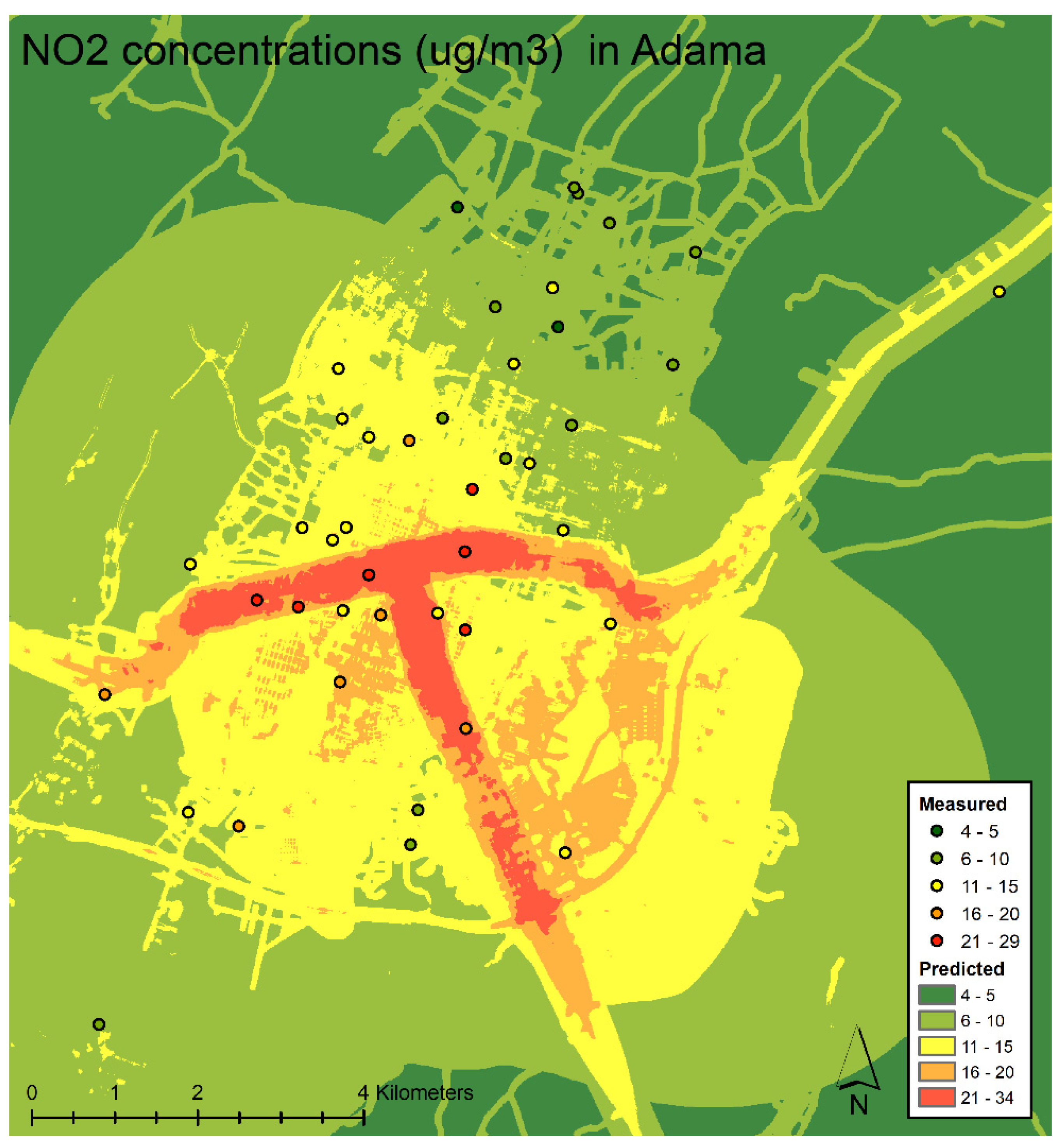
3.3.1. LUR for NO₂

In accordance with the ESCAPE protocol [40], univariate testing of all 59 geographical predictor variables was performed; of these, 19 were statistically significant (p-value > 0.05). Some of the statistically significant variables contained another variable. An example is primary roads with all buffer distances of 50, 100, 300, and 500 m being statistically significant. In such cases, the variables that had the highest correlation with the pollution concentration were selected to be tested in the multivariate model. For these variables, outer ring buffers were also calculated, univariately tested, and, if found statistically significant, included in the multivariate model. In total, 12 variables were added to the multivariate model, including two outer ring buffers (Prim_500_minus_300 and Res_3000_minus_1000), starting with the variable with the highest adjusted R₂. For variables to be kept in the model, the increase in adjusted R₂ needed to add more than 1%. The new variable should also conform to the prespecified direction and not change the direction of the effect for the already included predictor variables. After all the variables were tested, only four variables remained. Based on these, the variables’ residuals between the actual and predicted NO₂ levels were calculated for all measurement stations. The four remaining variables were then added to an intermediary model predicting the residuals. All variables had a statistical significance below 0.2, when predicting the residuals, and were therefore maintained.

This preliminary model was tested for influential observations and multicollinearity. The test showed no influential observations with the highest Cook’s D value being 0.255, but the VIF values were above 3 for two of the included variables, indicating the presence of multicollinearity. The variable with the highest VIF value (Distance to nearest transportation administration), was therefore excluded. This new model containing the three remaining variables was, again, tested for influential observations and multicollinearity. Here, neither the influential observations, with the highest Cook’s D value being 0.223, nor multicollinearity were observed. The final model was 4.044 + (0.00983*Primary road 300 m) + (2.99*10⁻⁶*Industrial area within 3000 m) + (0.0159*Road distance in meters within 50 m) (

Table 3. Variables and their coefficients (Beta) included in the final LUR model for NO₂.

Model Variable	Beta	SE	p-Value	VIF
Intercept	4.044	1.467	0.009
Primary road distance in meters within 300 m	0.00983	0.00141	2.62 × 10−8	1.123
Industrial area in m2 within 3000 m	2.99 × 10−6	5.23 × 10−7	1 × 10−6	1.095
Road distance in meters within 50 m	0.0159	0.00631	0.16	1.029

LUR = Land Use Regression. NO₂ = nitrogen dioxide. SE = Standard error. VIF = variance inflation factors.

). This model could explain 75.2% of the variance in NO₂ and had a RMSE of 3.03. No spatial autocorrelation was found when tested by Moran’s I with a nonsignificant Z-score of 0.208 (p-value 0.835).

When testing the internal validation of the model using a leave-one-out cross-validation, the average adjusted R² of these models was 0.75, and the RMSE was 2.99. With these adjusted R² values being very similar to that of our final model (0.75), a strong internal validity was indicated. A prediction map of NO₂ concentrations in the study area is presented in Figure 5.

3.3.2. LUR for NO_x

The NO_x model followed the same procedure as the NO₂ model. Univariate testing of the variables showed 22 statistically significant variables, of which three were outer ring buffers. In total, 12 variables were added to the multivariate model. Using the same criteria as described above, four variables were also included in the intermediary model, used to predict the residuals. After adding these in order of statistical significance, one variable (Residential area in m² within 1000 m) had a statistical significance above p = 0.2, the significance level set by the ESCAPE protocol [40]. This variable was excluded. The preliminary model was thereafter tested for influential observations and multicollinearity. The highest Cook’s D value was 0.38, which was well below the set limit of 1. The VIF value was also well below its established threshold of 3, indicating no multicollinearity. Thus, the preliminary model could be accepted. The final model was denoted as the following: 24.579 + (0.106 × Primary road distance in meters within 100 m) + (−0.00502 × Distance to closest transportation administration area) + (0.0468*Road distance in meters within 50 m) (

Table 4. Variables and their coefficients included in the final LUR model for NO_x.

Model Variable	Beta	SE	p-value	VIF
Intercept	24.579	4.614	0.000004
Primary road distance in meters within 100 m	0.106	0,0163	9.950 × 10−8	1.135
Distance to closest administration area	−0.00502	0.00135	0.000639	1.070
Road distance in meters within 50 m	0.0468	0.0200	0.0244	1.070

LUR = Land Use Regression. NO_x = nitrogen oxides. SE = Standard error. VIF = variance inflation factors.

). This model could explain 68.1% of the variance in the NO_x levels and had a RMSE of 9.43. No residual spatial autocorrelation was found when tested by Moran’s I with a nonsignificant Z-score of −0.699 (p-value 0. 484 > 0.05).

Again, the internal validity was tested with a leave-one-out cross-validation. The average adjusted R² of these validation models was 0.56 and the RMSE was 11.45. The difference between the cross-validation adjusted R² values and our final model´s R² indicate a somewhat weaker internal validity than that of the NO₂ model. Even so, this difference is still within the same magnitude as some of the models produced in the ESCAPE project [28]. A prediction map of the NO_x concentrations in the study area is presented in Figure 6.

The partial R² values, which is the variance explained given the other variables in the model, for each variable included in the two final models are presented in the Supplementary Materials (Tables S2 and S3).

4. Discussion

In this study, the measurements of NO_x and NO₂ were conducted at 43 locations over 6 days during two seasons. Based on these measurements, the LUR models were successfully developed for NO_x and NO₂. These models will be used in future epidemiological studies and health impact assessments in the Ethiopian city of Adama.

4.1. LUR Models

The LUR models developed in this study were able to explain 75.2% of the variance in NO₂ levels and 68.1% of the variance in NO_x levels, which can be considered as a good explanatory degree. With this, the models are suitable for use in local epidemiological studies. These levels of explanatory degree are also in the same magnitude as earlier models conducted in South Africa and Mauritania [18,19,34]. In Durban, South Africa, for instance, a LUR model could explain 73% of the variance of the NO_x levels (30). This model included similar geographical predictor variables as ours (major roads within 300 m, minor roads within 1000 m, and open space within 1000 m). However, the differences remain: the LUR model in Durban was developed in an area with numerous industrial sources, and Durban is a larger city than Adama. Another South African study from Western Cape Province developed a LUR model based on NO₂ measurements that were able to describe 76% of the annual variation [19]. In that study, separate models were also developed for the warm season (explaining 62% of the variance) and cold season (explaining 77% of the variance). In addition to variables related to roads and major roads, similar to those in our LUR model predicting NO₂ in Adama, the model also included the distance to bus stations and train stations, as well as grill places, within 1000 m. In Mauritania, a LUR model, studying NO₂ levels, was able to predict 68% of the variance (39). Similar to our Adama model, it included road variables, but in contrast, it also included variables related to population density. The Mauritanian model was based on 48 h of measurements, increasing the uncertainty of the results.

To relate the results to a European setting, our LUR models for NO_x and NO₂ can be compared with the 36 models developed by ESCAPE [28], which were able to explain 55% to 92% of the measured NO₂ and 49–91% of the measured NO_x. In our final NO_x and NO₂ models, we included predictor variables similar to those included in many of the models in ESCAPE, such as the distance to primary road, distance to the closest transport administration area, and distance to closest road and industrial area. These variables have also been used in other European studies to explain the spatial variability of urban air pollution [29,51].

Additionally, the LUR models created in Perth, Australia demonstrated stronger predictions for NO_x than NO₂ [52], but the opposite was seen for our final models in Adama. A LUR model developed for Taipei LUR showed similar results as in the Perth study, with a better performance for NO_x (81%) compared to NO₂ (74%) [53]. Similar to those used in our Adama model, these two studies also reported using predictor variables related to traffic intensity, industrial areas, and road length. Still, these study settings are quite different, making it difficult to know why our NO₂ model performed slightly better compared to the Perth and Taipei models. Possibly, the higher proportion of primary emissions in NO_x compared to NO₂ resulted in more spatial heterogeneity for NO_x. A greater spatial heterogeneity would require a higher level of monitoring data support for model predictions than with more homogeneous pollutants such as NO₂.

Our model showed that traffic, represented by the primary road and distance to the roads, correlates well with the estimated NO_x and NO₂ exposure. This is not surprising, considering the prevalent old and polluting vehicle fleet in the region.

When using LUR models to predict concentrations of NO_x or NO₂, it is important to consider the limitations for the model in predicting concentrations further away from places where the measurements were conducted. Predictions should only be made within the area that is covered by the measurement points. It is also important that the data for the prediction variables are complete at places where the concentrations are predicted, including buffer areas.

4.2. NO_x and NO₂ Measurement

In comparison to the few measurements conducted in similar African settings, our mean levels of NO₂ (13.1 µg/m³) were higher than those measured at Kaédi, a medium-sized town in Mauritania with a mean level of NO₂ of 5.3 µg/m³ [34]. Although, lower compared to a study from Western Cape Province, South Africa were mean NO₂ concentrations of 22 µg/m³ [19]. Our mean levels of NO_x (29.0 µg/m³) were somewhat lower compared to the mean NO_x levels of 36.4 μg/m³ in Durban [18]. Even so, worth mentioning is that the measurement site with the highest level of NO_x in Adama (86.5 μg/m³) was almost twice as high as that of Durban (50.9 μg/m³) [18], suggesting high local emissions at that site. It should also be noted that Adama is a relatively small city with NO_x levels that are higher than those recorded in a much larger city in a high-income country, such as Perth, with a mean level of NO_x of 18.7 µg/m³ [52]. This is likely due to the so-called super-emitters [54], as Ethiopia has become a dumping ground for the world’s old cars. Even so, the measured levels of NO₂ and NO_x in Adama remain in the lower spectrum of those reported in the ESCAPE project´s European cities, in which NO₂ ranged between 9.0 to 58.0 µg/m³ and NO_x from 19.0 to 101.0 µg/m³ [28].

In our study, traffic sites had the highest mean levels of NO_x (45.0 µg/m³) and NO₂ (17.5 µg/m³), whereas regional background sites had the lowest mean levels of both NO_x (15.6 µg/m³) and NO₂ (6.5 µg/m³). In comparison to the street background NO₂ levels measured in Kaédi, 7.0 µg/m³ of NO₂, our levels were more than six times higher [34]. However, the Kaédi measurements were conducted during the dry season only, which could influence their results. While we saw minimal differences between the dry and wet season, this might not be the case in Kaédi. Another difference between these studies is that the traffic intensity was described as low in Kaédi, which is not true for Adama. Furthermore, there is a higher uncertainty in the Kaédi measurements, as they were only conducted during a 48-h period, whereas ours were collected over 5 days. Regional background levels of NO₂ were also considerably higher in Adama compared to Kaédi (2.1 µg/m³). This could possibly be due to the extensive, episodic waste burning in Adama´s rural areas observed during the measurement campaigns. The fact that the ratios of NO₂/NO_x for the traffic sites were 0.39, 0.5 at the urban, and 0.46 at the regional background sites, confirmed that there likely were other NO sources, like episodic waste burning, near the regional sites.

4.3. Comparison to Active Measurements

4.3.1. Diurnal Trends

The spike of NO₂ and NO_x concentrations demonstrated in Figure 3 exemplifies the contribution of traffic exhaust to the overall air pollution levels, as this is typically when residents undergo their morning commutes to work or school. The early increases between 4 a.m. to 6 a.m. is probably related to traffic passing through Adama, as local traffic is not likely to contribute so strongly that early. Although an increase was present later in the day, a similar peak was not seen. It is possible that residents commute home at varying hours of the afternoon and evening. Additionally, the boundary layer is generally lower in the morning compared to the evening, which traps more pollutants close to the ground, increasing the measured concentrations.

4.3.2. Yearly Concentrations

While some variation existed between the years 2017 and 2018, the concentrations of NO₂ and NO_x appeared to be similar throughout the measurement period (Figure 4). Indeed, no substantial increase or decrease of the NO₂ and NO_x levels were seen. Due to a lack of continuous data points, however, we cannot draw conclusions relating to the seasonal trends (corresponding to the wet and dry seasons) based on this data.

4.3.3. Methodological Considerations

Comparisons of our measurements with the time-resolved data from the Ethiopian Meteorological Institute in Adama, featured in Figure 3 and Figure 4, warrant discussion. The reliability of the original data from this measuring station was likely affected by calibration issues, abrupt power outages, and irregular maintenance of the samplers. Daily averages in particular should be interpreted carefully, as the hours available for a specific day (i.e., hours occurring in the middle of the night vs. hours with a high traffic volume) will influence how high/low the daily averages are. Additionally, a large spike was seen on 10 August 2018 (Figure 4). This date corresponded to the timing of our 2018 measurement campaign, and we were not aware of any larger events that could explain this peak. Instead, it was likely caused by an isolated, unusually high local source, perhaps waste burning, near the active sampler. For these reasons, we emphasize that the NO₂ and NO_x data obtained from the Ethiopian Meteorological Institute in Adama only provided an indication of the NO₂ and NO_x concentrations in the area and should be interpreted with caution. Despite these concerns, it is important to compare our measurements from passive samplers to these available time-resolved measurements to understand the temporal trends in an otherwise data-sparse area.

4.4. Strengths and Limitations

Our study is the first air pollution model developed in Ethiopia and only among a few in Africa that can capture the spatial variability of NO_x and NO₂. It will be used to assess the air pollution exposure and will serve as an example for similar models in other areas such as Addis Ababa.

Regarding the land use variables, we were able to collect data on several of the most important variables. Reliable data on informal settlements was difficult to obtain; therefore, a degree of uncertainty, which is difficult to quantify, is expected for this variable. Additionally, marketplaces were discussed at the beginning of the project as an activity that could potentially contribute to increased levels of NO_x through combustion for cooking; however, this class was not included due to lack of reliable data. A specific class to assess solid waste burning was not able to be incorporated due to lack of data and its intermittent nature. Still, water bodies were included as a proxy to capture the larger, more frequently used waste burning sites. The solid burning was, however, more of an issue in our attempt to conduct a LUR model for particulate matter with a diameter less than 2.5 mm (PM_2.5) [47]. Data on the traffic intensity, which is considered to be important, was unfortunately not available. An attempt to gather this information was made using a local geotagger who collected data on the traffic intensity of several of roads in Adama, but the results were not considered representative enough for the different types of roads included in our study. The inclusion of variables that accurately reflect the additional land use practices, such as marketplaces, outdoor cooking, solid waste burning, and traffic intensity, will likely improve the development of LUR models in future studies.

The models were validated using leave-one-out cross-validation, a common validation tool for LUR models and standardized in the ESCAPE study [28]. The leave-one-out cross-validation method has been criticized for overestimating the predictive ability of LUR models, especially for models developed from a small number of measurements (less than 20) [55]. The RMSE error for both the NO_x (9.41 µg/m³) and NO₂ models were relatively low compared to the ranges of the measured concentrations (11.0 to 85.1 µg/m³ for NO_x and 5.0 to 28.8 µg/m³ for NO₂), indicating the usefulness of the models [28]. Another possible concern is whether our measurement sites were distributed well enough throughout the city, as some security issues arose in accessing certain areas. With a total of 41 measurement sites for the campaign in August 2018 and 42 sites in February 2019, however, we believe that we were able to capture the variance within most of the study area in relation to the identified emission sources (see Figure 1). Regarding the classification into the different types of stations, a cruder classification compared to the ESCAPE protocol had to be used, based on missing information about the traffic intensity and what was practically possible. The samplers needed to be guarded during the measurement campaign, and the samplers could thereby not be placed far away from the city center.

We originally performed three measurement campaigns, but only two were long enough to meet the requirements of the Ogawa protocol. When the first measurement campaign was launched in February 2018, Ethiopia declared a state of emergency. This delayed the campaign´s start and development of that measurement campaign, resulting in a measurement period of only 24 h; hence, it was not included in the LUR models. Still, the lessons learned at this time contributed to the success of the following measurement campaigns.

4.5. Implications

The annual mean level of NO₂ in Adama (13.1 µg/m³) was less than the WHO annual guideline of 40 μg/m³ [56], even though there is no national guideline for NO₂ and NO_x exposure in Ethiopia. Still, residents could likely be subjected to harmful levels of air pollution, depending on their proximity to certain roads, industries, or solid waste burning sites. Moreover, our LUR was shown to be a promising method to assess the spatial variation of NO_x and NO₂ in Adama. To date, only a few LUR models have been developed throughout the African continent; thus, our study adds to the application of LUR models for air pollution assessments. As LUR has recently started being used in low-income countries, this study is foundational to environmental epidemiology in such regions. Our models will, additionally, make a significant contribution to the evaluation of the effect of ambient air pollution on a variety of health outcomes in Adama through both epidemiological studies and health impact assessments. Specifically, our LUR models will be used to assess the outdoor NO_x and NO₂ exposures of women and children in an ongoing Adama birth cohort, which will investigate the health effects of air pollution exposure during gestation. Such epidemiological and health impact studies play an important role in motivating and supporting the development of air pollution policies and guidelines that, subsequently, contribute to improved public health.

5. Conclusions

Land Use Regression models for NO_x and NO₂ have been essential for the execution of epidemiological studies and health impact assessments in Europe and North America. The associations between exposure and health effects derived from such studies are simply not transferable to an African setting, since the air pollution sources and population characteristics are vastly different. Thus, it is crucial to conduct similar studies in African countries. Hindering this is the fact that air pollution data is often lacking, despite the health burden of air pollution falling disproportionately in this region. To address this gap, our study successfully developed LUR models for NO_x and NO₂ in Adama, Ethiopia. This will allow future epidemiological studies to be conducted, which will help raise awareness of air pollution exposure adverse health effects. Such findings can even inspire the creation of policies to improve the air quality and safeguard public health.

References

1. Cohen, A.J.; Brauer, M.; Burnett, R.; Anderson, H.R.; Frostad, J.; Estep, K.; Balakrishnan, K.; Brunekreef, B.; Dandona, L.; Dandona, R.; et al. Estimates and 25-year trends of the global burden of disease attributable to ambient air pollution: An analysis of data from the Global Burden of Diseases Study 2015. The Lancet 2017, 389, 1907–1918. [Google Scholar] [CrossRef] [Green Version]
2. Lelieveld, J.; Pozzer, A.; Giannadaki, D.; Evans, J.S.; Fnais, M. The contribution of outdoor air pollution sources to premature mortality on a global scale. Nature 2015, 525, 367–371. [Google Scholar] [CrossRef]
3. Burnett, R.; Chen, H.; Szyszkowicz, M.; Fann, N.; Hubbell, B.; Pope, C.A.; Apte, J.S.; Brauer, M.; Cohen, A.; Weichenthal, S.; et al. Global estimates of mortality associated with long-term exposure to outdoor fine particulate matter. Proc. Natl. Acad. Sci. 2018, 115, 9592. [Google Scholar] [CrossRef] [PubMed] [Green Version]
4. United States Environmental Protection Agency. Nitrogen Oxides (NOx) Why and How They Are Controlled; 456-F-99-006K; EPA: Durham, NC, USA, 1999. [Google Scholar]
5. Hänninen, O.; Knol, A.B.; Jantunen, M.; Lim, T.-A.; Conrad, A.; Rappolder, M.; Carrer, P.; Fanetti, A.-C.; Kim, R.; Buekers, J.; et al. Environmental burden of disease in Europe: Assessing nine risk factors in six countries. Environ. Health Perspect. 2014, 122, 439–446. [Google Scholar] [CrossRef] [PubMed] [Green Version]
6. Klepac, P.; Kukec, A.; Locatelli, I.; Korošec, S.; Künzli, N. Ambient air pollution and pregnancy outcomes: A comprehensive review and identification of environmental public health challenges. Environ. Res. 2018, 167, 144–159. [Google Scholar] [CrossRef] [PubMed]
7. Stockfelt, L.; Andersson, E.M.; Molnár, P.; Rosengren, A.; Wilhelmsen, L.; Sällsten, G.; Barregård, L. Long term effects of residential NOx exposure on total and cause-specific mortality and incidence of myocardial infarction in a Swedish cohort. Environ. Res. 2015, 142, 197–206. [Google Scholar] [CrossRef] [Green Version]
8. Urman, R.; McConnell, R.; Islam, T.; Avol, E.L.; Vora, H.; Linn, W.S.; Rappaport, E.B.; Gilliland, F.D.; Gauderman, W.J.; Lurmann, F.W. Associations of children’s lung function with ambient air pollution: Joint effects of regional and near-roadway pollutants. Thorax 2014, 69, 540–547. [Google Scholar] [CrossRef] [Green Version]
9. Enkhmaa, D.; Warburton, N.; Javzandulam, B.; Uyanga, J.; Khishigsuren, Y.; Lodoysamba, S.; Enkhtur, S.; Warburton, D. Seasonal ambient air pollution correlates strongly with spontaneous abortion in Mongolia. BMC Pregnancy Childbirth 2014, 14, 1–7. [Google Scholar] [CrossRef] [Green Version]
10. Lavigne, E.; Yasseen, I.I.I.A.S.; Stieb, D.M.; Hystad, P.; van Donkelaar, A.; Martin, R.V.; Brook, J.R.; Crouse, D.L.; Burnett, R.T.; Chen, H.; et al. Ambient air pollution and adverse birth outcomes: Differences by maternal comorbidities. Environ. Res. 2016, 148, 457–466. [Google Scholar] [CrossRef] [Green Version]
11. Li, L.; Laurent, O.; Wu, J. Spatial variability of the effect of air pollution on term birth weight: Evaluating influential factors using Bayesian hierarchical models. Environ. Health 2016, 15, 1–12. [Google Scholar] [CrossRef] [Green Version]
12. Malmqvist, E.; Liew, Z.; Källén, K.; Rignell-Hydbom, A.; Rittner, R.; Rylander, L.; Ritz, B. Fetal growth and air pollution - A study on ultrasound and birth measures. Environ. Res. 2017, 152, 73–80. [Google Scholar] [CrossRef] [Green Version]
13. Nobles, C.J.; Williams, A.; Ouidir, M.; Sherman, S.; Mendola, P. Differential effect of ambient air pollution exposure on risk of gestational hypertension and preeclampsia. Hypertens. (Dallas, Tex: 1979) 2019, 74, 384–390. [Google Scholar] [CrossRef]
14. Pedersen, M.; Stayner, L.; Slama, R.; Sørensen, M.; Figueras, F.; Nieuwenhuijsen, M.J.; Raaschou-Nielsen, O.; Dadvand, P. Ambient air pollution and pregnancy-induced hypertensive disorders: A systematic review and meta-analysis. Hypertension (0194911X) 2014, 64, 494–500. [Google Scholar] [CrossRef] [Green Version]
15. Lanzi, E.; Dellink, R.; Chateau, J. The sectoral and regional economic consequences of outdoor air pollution to 2060. Energy Econ. 2018, 71, 89–113. [Google Scholar] [CrossRef]
16. Schwela, D. Review of Urban Air Quality in Sub-Saharan Africa Region—Air Quality Profile of Ssa Countries; World Bank: Washington, DC, USA, 2012. [Google Scholar]
17. Martins, J.J.; Dhammapala, R.S.; Lachmann, G.; Galy-Lacaux, C.; Pienaar, J.J. Long-term measurements of sulphur dioxide, nitrogen dioxide, ammonia, nitric acid and ozone in southern Africa using passive samplers. S. Afr. J. Sci. 2007, 103, 336–342. [Google Scholar]
18. Muttoo, S.; Ramsay, L.; Brunekreef, B.; Beelen, R.; Meliefste, K.; Naidoo, R.N. Land use regression modelling estimating nitrogen oxides exposure in industrial south Durban, South Africa. Sci. Total. Environ. 2018, 610–611, 1439–1447. [Google Scholar] [CrossRef]
19. Toyib, O.; Mohamed, J.; Martin, R.; Rajen, N.; Roslynn, B.; Nino, K.; Ming, T.; Mark, D.; Kees de, H.; Dilys, B.; et al. A prospective cohort study on ambient air pollution and respiratory morbidities including childhood asthma in adolescents from the western Cape Province: Study protocol. BMC Public Health 2017, 17, 1–13. [Google Scholar] [CrossRef] [Green Version]
20. Mannucci, P.M.; Franchini, M. Health effects of ambient air pollution in developing countries. Int. J. Environ. Res. Public Health 2017, 14, 1048. [Google Scholar] [CrossRef]
21. African Development Bank. African Economic Outlook 2020. Available online: https://www.afdb.org/en/documents/african-economic-outlook-2020 (accessed on 1 November 2020).
22. United Nations Environment Programme. Addis Ababa City Air Quality Policy and Regulatory Situational Analysis. United Nations Environment Programme in collaboration with Envrionmental Compliance Insitute; 2018; Available online: https://www.eci-africa.org/wp-content/uploads/2019/05/Addis-Air-Quality-Policy-and-Regulatory-Situational-Analysis_Final_ECI_31.12.2018rev.pdf (accessed on 1 November 2020).
23. Bahino, J.; Yoboué, V.; Galy-Lacaux, C.; Adon, M.; Akpo, A.; Keita, S.; Liousse, C.; Gardrat, E.; Chiron, C.; Ossohou, M.; et al. A pilot study of gaseous pollutants’ measurement (NO2, SO2, NH3, HNO3 and O3) in Abidjan, Côte d’Ivoire: Contribution to an overview of gaseous pollution in African cities. Atmos. Chem. Phys. 2018, 18, 5173–5198. [Google Scholar] [CrossRef] [Green Version]
24. Hitchcook, G.; Conlan, B.; Kay, D.; Brannigan, C.; Newman, D. Air Quality and Road Transport—Impacts and Solutions; The Royal Automobile Clud Foundation for Motoring Ltd.: London, UK, 2014. [Google Scholar]
25. Amegah, A.K.; Agyei-Mensah, S. Urban air pollution in Sub-Saharan Africa: Time for action. Environ. Pollut. 2017, 220, 738–743. [Google Scholar] [CrossRef] [PubMed]
26. Solomon, A.O. The Role of Households in Solid Waste Management in East Africa Capital Cities. Ph.D. Thesis, Wageningen University, Wageningen, The Netherlands, 2011. [Google Scholar]
27. Eric, C.; Samuel, K. A narrative review on the human health effects of ambient air pollution in Sub-Saharan Africa: An urgent need for health effects studies. Int. J. Environ. Res. Public Health 2018, 15, 427. [Google Scholar] [CrossRef] [Green Version]
28. Beelen, R.; Hoek, G.; Vienneau, D.; Eeftens, M.; Dimakopoulou, K.; Pedeli, X.; Tsai, M.-Y.; Künzli, N.; Schikowski, T.; Marcon, A.; et al. Development of NO2 and NOx land use regression models for estimating air pollution exposure in 36 study areas in Europe–The ESCAPE project. Atmos. Environ. 2013, 72, 10–23. [Google Scholar] [CrossRef]
29. Ryan, P.H.; LeMasters, G.K. A review of land-use regression models for characterizing intraurban air pollution exposure. Inhal. Toxicol. 2007, 19, 127–133. [Google Scholar] [CrossRef] [PubMed] [Green Version]
30. Madsen, C.; Håberg, S.E.; Nafstad, P.; Nystad, W.; Gehring, U.; Meliefste, K.; Brunekreef, B.; Lødrup Carlsen, K.C. Comparison of land-use regression models for predicting spatial NOx contrasts over a three year period in Oslo, Norway. Atmos. Environ. 2011, 45, 3576–3583. [Google Scholar] [CrossRef]
31. Wang, R.; Henderson, S.B.; Sbihi, H.; Allen, R.W.; Brauer, M. Temporal stability of land use regression models for traffic-related air pollution. Atmos. Environ. 2013, 64, 312–319. [Google Scholar] [CrossRef]
32. Jerrett, M.; Arain, M.A.; Kanaroglou, P.; Beckerman, B.; Crouse, D.; Finkelstein, N.; Gilbert, N.L.; Brook, J.R.; Finkelstein, M.M. Modeling the intraurban variability of ambient traffic pollution in Toronto, Canada. J. Toxicol. Environ. Health Part A: Current Issues 2007, 70, 200–212. [Google Scholar] [CrossRef]
33. Choi, G.; Bell, M.L.; Lee, J.T. A study on modeling nitrogen dioxide concentrations using land-use regression and conventionally used exposure assessment methods. Environ. Res. Lett. 2017, 12, 044003. [Google Scholar] [CrossRef] [Green Version]
34. Sirak Zenebe, G.; Danielle, V.; Christian, F.; Hâmpaté, B.; Guéladio, C.; Ming-Yi, T. Spatial air pollution modelling for a West-African town. Geospat. Health 2015, 10. [Google Scholar] [CrossRef] [Green Version]
35. World Health Organization. Ambient Air Pollution: A Global Assessment of Exposure and Burden of Disease; World Health Organization: Geneva, Switzerland, 2016. [Google Scholar]
36. Ethiopia Demographics. Available online: https://www.worldometers.info/demographics/ethiopia-demographics/ (accessed on 11 October 2020).
37. Messay, M.; Degefa, T.; Gezahegn, A. Description of long-term climate data in Eastern and Southeastern Ethiopia. Data in Brief 2017, 12, 26–36. [Google Scholar] [CrossRef]
38. Adama City Administrative Office. Adama City Administrative Office Report; Adama City Administrative Office: Adama, Ethiopia, 2019; Unpublished. [Google Scholar]
39. Ayehu, F.M. Evaluation of Traffic Congestion and Level of Service at Major Intersections in Adama City. Master’s Thesis, Addis Ababa University, Addis Ababa, Ethiopia, 2015. [Google Scholar]
40. Brunekreef, B. ESCAPE Exposure Assessment Manual. Available online: http://www.escapeproject.eu/manuals/ESCAPE-Study-manual_x007E_final.pdf (accessed on 1 January 2017).
41. Hagenbjörk-Gustafsson, A.; Tornevi, A.; Forsberg, B.; Eriksson, K. Field validation of the Ogawa diffusive sampler for NO2 and NOx in a cold climate. J. Environ. Monit. 2010, 12, 1315–1324. [Google Scholar] [CrossRef] [PubMed]
42. Malmqvist, E.; Olsson, D.; Hagenbjörk-Gustafsson, A.; Forsberg, B.; Mattisson, K.; Stroh, E.; Strömgren, M.; Swietlicki, E.; Rylander, L.; Hoek, G.; et al. Assessing ozone exposure for epidemiological studies in Malmö and Umeå, Sweden. Atmos. Environ. 2014, 94, 241–248. [Google Scholar] [CrossRef] [Green Version]
43. Tseganesh, M. Adama City Final Structure; Adama City Urban Land Development and Management Office: Adama, Ethiopia, 2019. [Google Scholar]
44. Corporation Satellite Imaging. Sensors Used in Satellite Imaging. Available online: https://www.satimagingcorp.com/satellite-sensors/ (accessed on 1 January 2020).
45. Hoek, G.; Beelen, R.; de Hoogh, K.; Vienneau, D.; Gulliver, J.; Fischer, P.; Briggs, D. A review of land-use regression models to assess spatial variation of outdoor air pollution. Atmos. Environ. 2008, 42, 7561–7578. [Google Scholar] [CrossRef]
46. Open Street Map. Available online: www.openstreetmap.org/ (accessed on 1 January 2020).
47. Asmamaw, A.; Kristoffer, M.; Axel, E.; Erik, A.; Geremew, S.; Bezatu, M.; Abebe Genetu, B.; Abraham, A.; Ebba, M.; Christina, I. Air pollution measurements and land-use regression in urban Sub-Saharan Africa using low-cost sensors—possibilities and pitfalls. Atmosphere 2020, 11, 1357. [Google Scholar] [CrossRef]
48. Chang, T.-Y.; Liang, C.-H.; Wu, C.-F.; Chang, L.-T. Application of land-use regression models to estimate sound pressure levels and frequency components of road traffic noise in Taichung, Taiwan. Environ. Int. 2019, 131. [Google Scholar] [CrossRef] [PubMed]
49. Lee, M.; Brauer, M.; Wong, P.; Tang, R.; Tsui, T.H.; Choi, C.; Cheng, W.; Lai, P.-C.; Tian, L.; Thach, T.-Q.; et al. Land use regression modelling of air pollution in high density high rise cities: A case study in Hong Kong. Sci. Total. Environ. 2017, 592, 306–315. [Google Scholar] [CrossRef] [PubMed] [Green Version]
50. Zhang, Z.; Wang, J.; Hart, J.E.; Laden, F.; Zhao, C.; Li, T.; Zheng, P.; Li, D.; Ye, Z.; Chen, K. National scale spatiotemporal land-use regression model for PM2.5, PM10 and NO2 concentration in China. Atmos. Environ. 2018, 192, 48–54. [Google Scholar] [CrossRef]
51. Dons, E.; Van Poppel, M.; Int Panis, L.; De Prins, S.; Berghmans, P.; Koppen, G.; Matheeussen, C. Land use regression models as a tool for short, medium and long term exposure to traffic related air pollution. Sci. Total. Environ. 2014, 476–477, 378–386. [Google Scholar] [CrossRef] [PubMed]
52. Dirgawati, M.; Barnes, R.; Wheeler, A.J.; Arnold, A.-L.; McCaul, K.A.; Stuart, A.L.; Blake, D.; Hinwood, A.; Yeap, B.B.; Heyworth, J.S. Development of land use regression models for predicting exposure to NO2 and NOx in Metropolitan Perth, Western Australia. Environ. Model. Softw. 2015, 74, 258–267. [Google Scholar] [CrossRef]
53. Lee, J.-H.; Wu, C.-F.; Hoek, G.; de Hoogh, K.; Beelen, R.; Brunekreef, B.; Chan, C.-C. Land use regression models for estimating individual NOx and NO2 exposures in a metropolis with a high density of traffic roads and population. Sci. Total. Environ. 2014, 472, 1163–1171. [Google Scholar] [CrossRef]
54. Abera, A.; Friberg, J.; Isaxon, C.; Jerrett, M.; Malmqvist, E.; Sjöström, C.; Taj, T.; Vargas, A.M. Air quality in Africa: Public health implications. Annu. Rev. Public Health 2021, 42, null. [Google Scholar] [CrossRef]
55. Wang, M.; Beelen, R.; Basagana, X.; Becker, T.; Cesaroni, G.; de Hoogh, K.; Dedele, A.; Declercq, C.; Dimakopoulou, K.; Eeftens, M.; et al. Evaluation of land use regression models for NO2 and particulate matter in 20 European study areas: The ESCAPE project. Environ. Sci. Technol. 2013, 47, 4357–4364. [Google Scholar] [CrossRef] [PubMed]
56. World Health Organization. WHO Air Quality Guidelines for Particulate Matter, Ozone, Nitrogen Dioxide and Sulfur Dioxide: Global Update 2005: Summary of Risk Assessment; World Health Organization: Geneva, Switzerland, 2006. [Google Scholar]
Figure 1. The location of Adama on the East African continent, and the air sampling measurement sites and land use classes included in the LUR models.
Atmosphere 12 00519 g001
Figure 2. Photo of Ogawa badge in its rain protection from one of the NOx and NO2 sampling sites.
Atmosphere 12 00519 g002
Figure 3. Diurnal trend of NO2 and NOx in Adama City, averaged from 13 days with complete data.
Atmosphere 12 00519 g003
Figure 4. Yearly concentrations of NO2 and NOx in Adama City.
Atmosphere 12 00519 g004
Figure 5. Prediction map of the NO2 concentrations in a 10-m grid over Adama based on the developed LUR model. The measured levels of NO2 are presented by dots.
Atmosphere 12 00519 g005
Figure 6. Prediction map of NOx concentrations in a 10-m grid over Adama based on the developed LUR model. Measured levels of NOx are presented by dots. Grey marks areas were the model predicted zero or below.
Atmosphere 12 00519 g006