Article

Climatic Effects of Spring Mesoscale Oceanic Eddies in the North Pacific: A Regional Modeling Study

1
Key Laboratory of Meteorological Disaster/KLME/ILCEC/CIC-FEMD, Nanjing University of Information Science & Technology, Nanjing 210044, China
2
School of Atmospheric Sciences, Nanjing University of Information Science & Technology, Nanjing 210044, China
*
Author to whom correspondence should be addressed.
Atmosphere 2021, 12(4), 517; https://doi.org/10.3390/atmos12040517
Submission received: 13 February 2021 / Revised: 14 April 2021 / Accepted: 17 April 2021 / Published: 19 April 2021
(This article belongs to the Section Climatology)

Abstract

:
A high-resolution atmospheric model of the Weather Research and Forecast (WRF) is used to investigate the climatic effects of mesoscale oceanic eddies (OEs) in the North Pacific (NPac) in spring and the respective effects of OEs in the northern NPac associated with the Kuroshio Extension (KE) and of OEs in the southern NPac related to the subtropical countercurrent. Results show that mesoscale OEs in the NPac can strengthen the upper-level ridge (trough) in the central (eastern) subtropical NPac, together with markedly weakened (strengthened) westerly winds to its south. The mesoscale OEs in the whole NPac act to weaken the upper-level storm track and strengthen lower-level storm activities in the NPac. However, atmospheric responses to the northern and southern NPac OEs are more prominent. The northern NPac OEs can induce tropospheric barotropic responses with a tripole geopotential height (GPH) anomaly pattern to the north of 30° N, while the OEs in both the northern and southern NPac can enhance the upper-level ridge (trough) in the central (eastern) subtropical NPac. Additionally, the northern NPac OEs can shrink the lower-level subtropical high and weaken the easterly trade winds at the low latitudes, while the southern NPac OEs result in a southward shift of the lower-level subtropical high and an eastward shift of the upper-level westerly jet stream. The southern and northern NPac OEs have similar effects on the storm track, leading to an enhanced lower-level storm track over the KE via moistening the atmospheric boundary layer; and they can also exert significant remote influences on lower- and upper-level storm activities over the Northeast Pacific off the west coast of North America. When the intensities of OEs are doubled in the model, the spatial distribution of atmospheric responses is robust, with a larger and more significant magnitude. Additionally, although OEs are part of the mesoscale oceanic processes, the springtime OEs play an opposite role in mesoscale sea-surface temperature anomalies. These findings point to the potential of improving the forecasts of extratropical springtime storm systems and the projections of their responses to future climate change, by improving the representation of ocean eddy-atmosphere interaction in forecast and climate models.

1. Introduction

Air-sea interactions have always been an important topic in climate research. In the extratropics, they are often characterized by a negative correlation between surface wind speed (SWS) and sea surface temperature (SST) on a basin scale, indicative of the atmospheric role in forcing the ocean. Air-sea coupling allows the ocean to respond to the internal variability of atmosphere through air-sea heat fluxes, and the atmosphere would in turn experience reduced surface thermal damping due to the SST adjustment, which increases the low-frequency atmospheric variation [1]. In contrast, a positive correlation between SWS and SST has been identified on small scales. SWS is found to be locally higher over warm water and lower over cool water, which is indicative of the active oceanic role in forcing the atmosphere [2,3,4,5,6,7]. Many studies have focused on oceanic mesoscale systems of 50–500 km, such as ocean fronts, mesoscale oceanic eddies (OEs), and tropical instability waves. However, the definitions of the spatial scale of these mesoscale processes are flexible in actual research.
Atmospheric responses to mesoscale SST anomalies (SSTAs) have attracted extensive attention, especially for the western boundary regimes of the Northern Hemisphere. The Kuroshio and Gulf Stream, two powerful warm currents that are constantly accompanied by mesoscale OEs, not only transport a large amount of heat to the mid latitudes, but also cause obvious SST meridional gradients (and thus ocean fronts), resulting in significant mesoscale air-sea interactions along their paths [8,9,10,11,12,13]. Nakamura et al. [14] pointed out that the location of a mid-latitude storm track in the Northern Hemisphere was closely related to ocean fronts in the western boundary regimes. Based on a regional atmospheric model, Taguchi et al. [15] revealed that mesoscale SSTAs over the Kuroshio-Oyashio Extension could enhance the local turbulent heat fluxes, water vapor flux, meridional temperature gradient, and the baroclinicity of the upper-level atmosphere, which ultimately strengthens the local cyclone activities and anchors the storm track in the North Pacific (NPac). Similar storm track responses can also be found over the Northwest Atlantic [16]. Thus, mesoscale SSTAs have significant impacts on storm activities, but probably through different mechanisms [17].
Owing to the development of OEs’ detection and tracking algorithms, the effects of OEs on the overlying atmosphere have been widely studied. Observational and numerical studies have revealed that these OEs can significantly affect the atmospheric boundary layer [18,19,20,21]. Frenger et al. [22] first conducted a statistical study based on more than 600,000 transient OEs in the Southern Ocean and found that cyclonic (anticyclonic) eddies were accompanied by decreased (increased) near-surface wind speed, heat fluxes, cloud fraction, and rainfall, but these well-established local impacts have regional differences and seasonal variation, probably due to variations in background SST, atmospheric stability, and near-surface wind [23,24,25]. Ma et al. [26,27] investigated the atmospheric responses to OEs in the Kuroshio Extension (KE) and related seasonal variation characteristics. They revealed distinct seasonal variations in SWS and heat flux responses, characterized by much stronger effects in the cold seasons (winter and spring) than in the warm seasons (summer and autumn). They also found that these atmospheric responses could penetrate beyond the atmospheric boundary layer. However, atmospheric responses to mesoscale SSTAs over the Agulhas Return Current are only limited to the boundary layer [28]. More recently, Ma et al. [29,30] investigated the climatic effects of wintertime mesoscale SSTAs in the KE and found that the removal of mesoscale SSTAs in the KE could exert a significant distant influence on winter rainfall variability and storm track in the downstream eastern NPac. However, these removed SSTAs were induced by both OEs and other mesoscale systems. For instance, Foussard et al. [31] revealed that OEs of about 500 km could shift the storm track poleward by about 1000 km through eddy-induced diabatic heating based on an idealized atmospheric model.
The potential climatic responses to mesoscale OEs in real oceans, however, are not sufficiently investigated. Given that the number of OEs in the NPac reaches its maximum in spring, which can also cause significant local atmospheric responses [32,33,34], we aim to investigate the effects of OEs in the NPac on large-scale atmospheric circulation and storm track in spring by conducting a series of numerical simulations based on realistic distributions of OEs without any other mesoscale processes (such as meanders or SST fronts), which differs from many previous studies (e.g., Putrasahan et al. [35]; Seo et al. [36]; Ma et al. [29,30]; Jia et al. [37]). As there are two noteworthy eddy-enriched regions in the NPac which are related to the KE and the subtropical countercurrent, respectively [32,34,38,39], different effects of OEs in the northern (related to the KE) and southern (related to the subtropical countercurrent) NPac regions are examined in this study. The remainder of the paper is organized as follows. We introduce the dataset, model, and configurations of the simulation in Section 2. Then, we compare the control run with observations and investigate the effects of OEs in the whole, northern, and southern NPac on the atmospheric circulations and storm track, respectively, in Section 3. A summary of our major findings and a discussion are given in Section 4.

2. Data and Methods

2.1. Observational Data

We used the SST field from the Optimal Interpolation SST Analysis version 2 (OISSTV2; available online at ftp://ftp2.psl.noaa.gov/Datasets/noaa.oisst.v2.highres (accessed on 25 September 2020); Reynolds et al. [40]), the sea-level anomaly (SLA) data from the Archiving Validation and Interpretation of Satellite (AVISO; available online at https://www.aviso.altimetry.fr/en/data (accessed on 9 September 2020)), and daily gridded ocean wind vectors from the Quick Scatterometer (QuikSCAT) Level-3 (available online at http://data.remss.com/qscat/ (accessed on 25 September 2020); Liu et al. [41]). These datasets are all on a 0.25° grid. We also used the Climate Forecast System Reanalysis (CFSR; available online at https://rda.ucar.edu/datasets/ (accessed on 29 August 2020)) 6-hourly reanalysis dataset with 37 vertical isobaric layers on a 0.5° grid and heat fluxes (latent and sensible heat fluxes) at the resolution of 0.313° latitude by 0.313° longitude, which have been widely used [26,27,42,43]. Considering the relatively short records of near-surface winds from the QuikSCAT (from June 1999 to November 2009), we only used the data from 2003 to 2008.
In addition, the database of trajectories of global OEs version 2 (available online at http://wombat.coas.oregonstate.edu/eddies (accessed on 9 September 2020); Chelton et al. [44])) is used, including all the needed information of each eddy, such as its individual center, size, polarity, intensity, and amplitude in detail from January 1993 to April 2015. In this new version, OEs have a larger amplitude, smaller radii, and higher rotational speeds in comparison with those in the previous versions [45,46,47].

2.2. Model and Experimental Design

2.2.1. Model Description

The Weather Research and Forecasting (WRF) Model version 3.8.1, developed by the National Center for Atmospheric Research (NCAR), is a fully compressible and non-hydrostatic model and has shown excellent simulation capabilities in mesoscale and regional climate simulation studies. More details about this model can be found in Skamarock et al. [48]. In this study, the model with initial and lateral boundary conditions derived from the NCEP Global Forecast System Final Operational Global (GFS FNL; available online at https://rda.ucar.edu/datasets/ds083.2/ (accessed on 29 August 2020)). An analysis with 6-hourly temporal resolution is configured for a domain that covers the whole NPac (125° E–115° W, 0°–62.5° N). The configuration used in this study has 30 vertical levels that are unevenly distributed from the surface to 50 hPa (top of the model) and with a spacing of 20 km based on a Mercator projection. The physical options include the Kain–Fritsch (KF) cumulus scheme, Lin et al.’s (1983) microphysics scheme, the Noah land surface scheme, the Yonsei University (YSU) planetary boundary layer (PBL) scheme, the Rapid Radiative Transfer Model for General Circulation Models (RRTMG), and the Goddard scheme for longwave and shortwave radiation, all of which have been widely used in previous studies [28,29,49,50].

2.2.2. Experimental Design

Eddy kinetic energy (EKE) in the ocean is defined as u 2 + v 2 2 , u = g f   h y     and v = g f   h x , where h′, u′, and v′ are the 40–300 day filtered SLA and the corresponding zonal and meridional geostrophic current anomalies, respectively. EKE can provide a good representation of the intensity of OE activities. Figure 1 shows its climatological distribution in the NPac from 2003 to 2008. The largest EKE from the ocean occurs in the KE region, extending eastward to the International Dateline, and the second largest EKE is mainly related to the subtropical ocean front and countercurrent, which extends eastward to the west of the Hawaiian Islands [27,32,34,39,51]. Here, we used the latitude of 25° N (red dotted line in Figure 1) to roughly divide the NPac into two parts: the northern part (north of 25° N), mainly associated with OEs in the Kuroshio and KE, and the southern part (south of 25° N), related to eddies in the subtropical countercurrent. In this study, a series of numerical experiments (Table 1) are conducted, including a control experiment (CTL), a spatially smoothed-SST experiment (SmthSST), and three sensitivity experiments to explore the climatic effects of OEs in the whole, northern, and southern NPac in spring (from March to May, or MAM), respectively. All simulations are integrated for four months from 00 UTC 1 February to 00 UTC 1 June for the six years from 2003 to 2008 (serving as six ensemble members). The model outputs are stored at the interval of 24 h, and those in the first month were considered as the model spin-up and were not used in the analysis.
Daily observed SSTs from the OISSTV2 with a resolution as high as 0.25° in both latitude and longitude are used as the lower boundary condition for CTL, which can well resolve the fine structures of oceanic fronts and eddies. In SmthSST, a daily SST field is spatially smoothed using a two-dimensional sliding lowpass Gaussian filter to eliminate mesoscale SST variability with a spatial scale smaller than 500 km; the size of the filter window at any grid can be determined by the cutoff wavelength (set as 500 km, as used in this study, supposing the filter window size is m (zonal) by n (meridional)). In this filter, the contribution of each pixel is weighted by a Gaussian curve, which is symmetric with regard to the center pixel, and the standard deviation of this Gaussian curve is defined as cut   off   wavelength res × ( 2 ×   π ), where res denotes the grid spacing of the sample points. In this study, the res on the fixed grid of the observational data was calculated as 1 2 × cut   off   wavelength m   1 + cut   off   wavelength n   1 , and the res on the WRF model grid was fixed at 20 km. A more detailed description of this filter can be found in Greene et al. [52]. Thus, we obtained SST ¯ by applying this filter, and the residual SST = SST     SST ¯ . Note that SST contains all mesoscale processes, including meanders and fronts. In the OE dataset mentioned above, the radius and position of each OE are recorded. Starting from the center of each OE, the corresponding SST is retained if the surrounding grid is within its radius; otherwise, it is excluded. Finally, the SSTA associated with the OEs only can be obtained, and three experiments, namely, EddySSTA, EddySSTA + N25N, and EddySSTA + S25N, are conducted to reveal the effects of the OEs in the whole, northern, and southern NPac, respectively. EddySSTA is the same as SmthSST, except that the SSTAs associated with OEs in the whole NPac are superimposed on the smoothed SST field. EddySSTA + N25N and EddySSTA + S25N are similar to EddySSTA, except that SSTAs only superimposed on the smoothed SST field to the north and south of 25° N, respectively. Therefore, the regional climatic effects of OEs over the whole, northern, and southern NPac can be quantitatively revealed by the differences between the outputs of SmthSST and those of EddySSTA, EddySSTA + N25N, and EddySSTA + S25N, respectively. For example, Figure 2 shows the smoothed SST field and SSTAs associated with OEs in the whole, northern, and southern NPac at 00 UTC on 1 March 2004. We can see that a large number of OEs occur in the NPac, especially in the Kuroshio and KE, and the OEs to the south of the Kuroshio and KE are relatively weak, which is consistent with the EKE distribution in Figure 1.

2.2.3. Empirical Monte Carlo Significance Test

In this study, the Empirical Monte Carlo (EMC) test is used to test the statistical significance of differences between different experiments because the atmospheric variables do not satisfy the normal distribution and have a strong continuity. In the EMC test, the variable at each grid box is randomly sorted 1000 times, and the 5% quantile is chosen as the 0.05 significance level.

3. Results

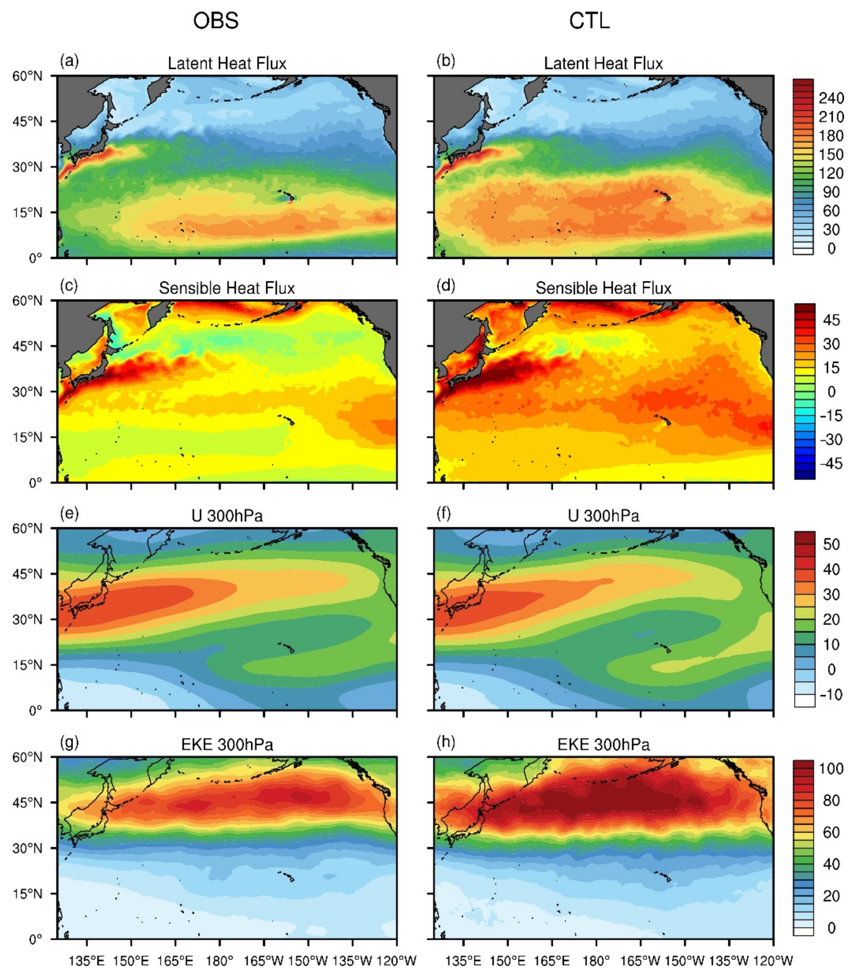
3.1. Model Validation

Figure 3 compares the simulated MAM-mean surface latent heat flux (LHF) and the sensible heat flux (SHF) with the CFSR products. In spring, LHF is the strongest in the zonally elongated region along the KE, and with a relatively weaker elongated maximum in LHF to the south of Hawaii along the Intertropical Convergence Zone (ITCZ) (Figure 3a). Similarly, SHF also shows the most prominent peak in the KE and the east coast of Japan, with another weaker center in the eastern NPac of the low latitudes (Figure 3c). We found that the LHF averaged over the KE (130°–165° E, 15°–25° N) is 147.8 and 165.2 W m−2 in observations and the model, respectively, while the respective LHF averaged over the subtropical region (135° E–150° W, 10°–25° N) is 144.9 and 174.3 W m−2, indicating a ~15% overestimation of the LHF in the model. The model also significantly overestimates SHF, especially over the low latitudes of the eastern NPac (Figure 3b,d). Such overestimated surface turbulent heat fluxes (SHF and LHF) have also been reported in many previous wintertime model simulations [53,54]. Overall, the WRF model can roughly and reasonably reproduce the spatial patterns of SHF and LHF. The simulated upper-level zonal winds (Figure 3f) are generally consistent with the observations (Figure 3e). The prevailing westerly winds in the mid latitudes extend from the western to the eastern NPac with a maximum of up to 40 m s−1 over South Japan. The model also captures the springtime upper-level storm track extending across the NPac well, with its maximum center above the central NPac, except for a slightly overestimated EKE in the atmosphere (defined as u 2 + v 2 2 , where the prime denotes the synoptic-scale component with a time scale of 2.5–6.0 days extracted by the butterworth band-pass filter) in the central NPac, Asia, and the west coast of North America (Figure 3g–h).
To verify the positive correlation between small-scale SSTAs and near-surface wind speed in the literature [55,56,57,58,59], we randomly selected the averaged SSTAs and near-surface wind speed anomalies in March 2003. Here, the anomalies are filtered by the spatial Gaussian filter, and the linear regression coefficients of near-surface wind speed anomalies onto SSTAs are regarded as the coupling strength. Figure 4a,c shows the spatial distributions of observational and simulated SSTAs and near-surface wind speed anomalies in the NPac, respectively. Positive (negative) SSTAs correspond well to positive (negative) near-surface wind speed anomalies in the observations, and the coupling strength in the KE (black dashed box in Figure 4a) is about 0.46 m s−1 °C−1 (Figure 4b). However, the simulated near-surface wind speed anomalies are much weaker than those in the observations; that is, an SSTA of 1 °C only induced a wind speed anomaly of about 0.24 m s−1 (Figure 4d). These results are consistent with the finding of Gao et al. [60], which suggested that the simulated coupling strength is 0.22 m s−1 °C−1 over the Kuroshio and KE, only half the observed strength of 0.44 m s−1 °C−1. To the south of 25° N (130°–165° E, 15°–25° N), the coupling strength between SSTA and surface wind anomalies in the WRF model and the observations are 0.20 and 0.37, respectively (figure not shown). This underestimated coupling strength in the boundary layer is mainly related to the PBL parameterization scheme in the model [28,58,61], and this coupling in SSTA and surface wind is still smaller than the observed coupling by a factor of 2–4 for all Numerical Weather Prediction (NWP) and climate models [6].
Overall, the WRF can reasonably simulate the springtime surface heat fluxes, large-scale atmospheric circulations, and storm track over the NPac, as well as the positive wind-SST relationship on small scales, but with a weaker coupling strength. Thus, we will use the model to investigate the climatic effects of mesoscale OEs next.

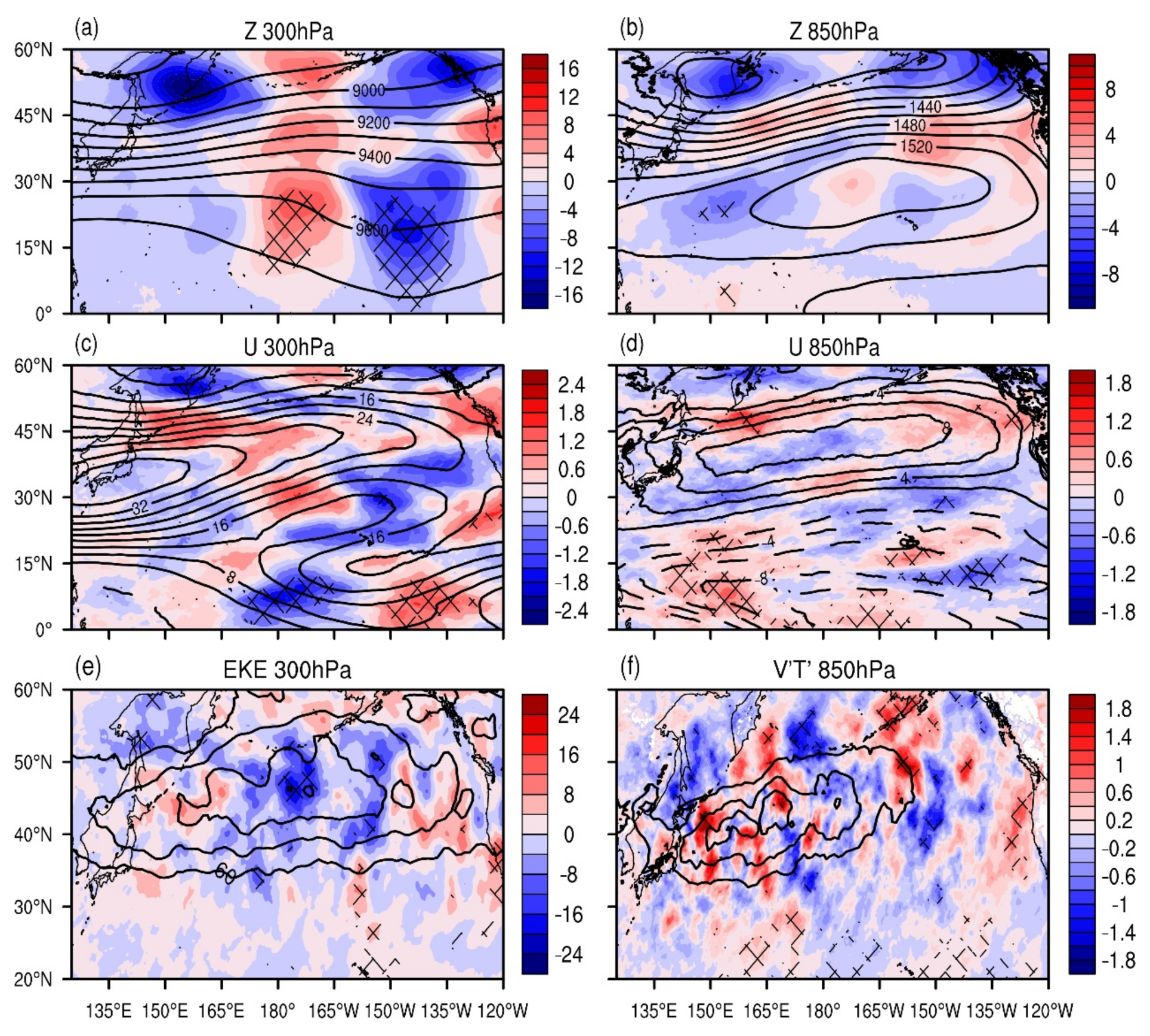
3.2. Impacts of OEs in the Whole NPac

Figure 5 shows the MAM-mean differences of geopotential heights (GPH), zonal winds, and storm track in the upper and lower levels between EddySSTA and SmthSST over the whole NPac. The NPac storm track in the upper and lower levels is measured by a transient EKE in the atmosphere at 300 hPa and a poleward heat flux v T at 850 hPa, respectively, where the prime denotes the synoptic-scale component with a time scale of 2.5–6.0 days extracted by the butterworth band-pass filter [15,62]. Remarkable positive 300-hPa GPH anomalies occur over the central subtropical NPac near the International Dateline (Figure 5a), indicating that mesoscale OEs can help maintain and strengthen the upper-level ridge there. This enhanced ridge is conducive to reducing GPH with cold advection anomalies in the downstream region of the central NPac and thus enhances the trough. However, the OE-induced GPH anomalies in the mid-to-high latitudes differ from those in the low latitudes, with two negative centers over the Sea of Okhotsk and Alaska, respectively. This anomaly pattern acts to decrease the upper-level GPH over the east coast of Asia and the west coast of North America, respectively. Meanwhile, similar negative GPH anomalies can be found at 850 hPa over the Gulf of Alaska and the east coast of Asia in high latitudes, but with relatively weak anomalies, indicative of an equivalent barotropic response to OEs (Figure 5b). In addition, evident negative GPH anomalies induced by OEs occur to the west of the Pacific subtropical high (PSH), suggesting an eastward shift of the lower-level subtropical high.
The westerly wind significantly decreased (increased) over the central (eastern) tropical Pacific (Figure 5c), corresponding to the strengthened trough (ridge) in the subtropical NPac (Figure 5a). Meanwhile, zonal wind changes at 850 hPa (Figure 5d) are similar to those at 300 hPa in the northern NPac (north of 25° N); however, the lower-level zonal winds increased (decreased) over the western (eastern) tropical NPac (south of 15° N), which is closely related to the negative GPH anomalies to the west of the PSH (Figure 5b). As the Kuroshio and KE are two important regions for cyclogenesis in the NPac, OEs in these regions may have impacts on storm activities and thus their associated storm track. When the OEs are included in the model, the 850-hPa storm track over the KE and its downstream region (i.e., the west coast of North America) are largely enhanced (Figure 5f). These amplification effects of OEs on the main body of the lower-level storm track and the downstream west coast of North America in spring are quite similar to the effects of wintertime mesoscale SSTAs in the whole NPac [29,30]. However, such effects of OEs are relatively weaker than ocean fronts, which is likely due to their spatial randomness [15,16,53,54]. In the upper troposphere, OEs induce significant negative EKE anomalies over the central NPac (Figure 5e) and thus weaken the upper-level storm track, which is consistent with Foussard et al. [31], although their model domain is close to the Antarctic Circumpolar Current. Therefore, mesoscale OEs in the NPac can affect both the lower- and upper-level storm track.

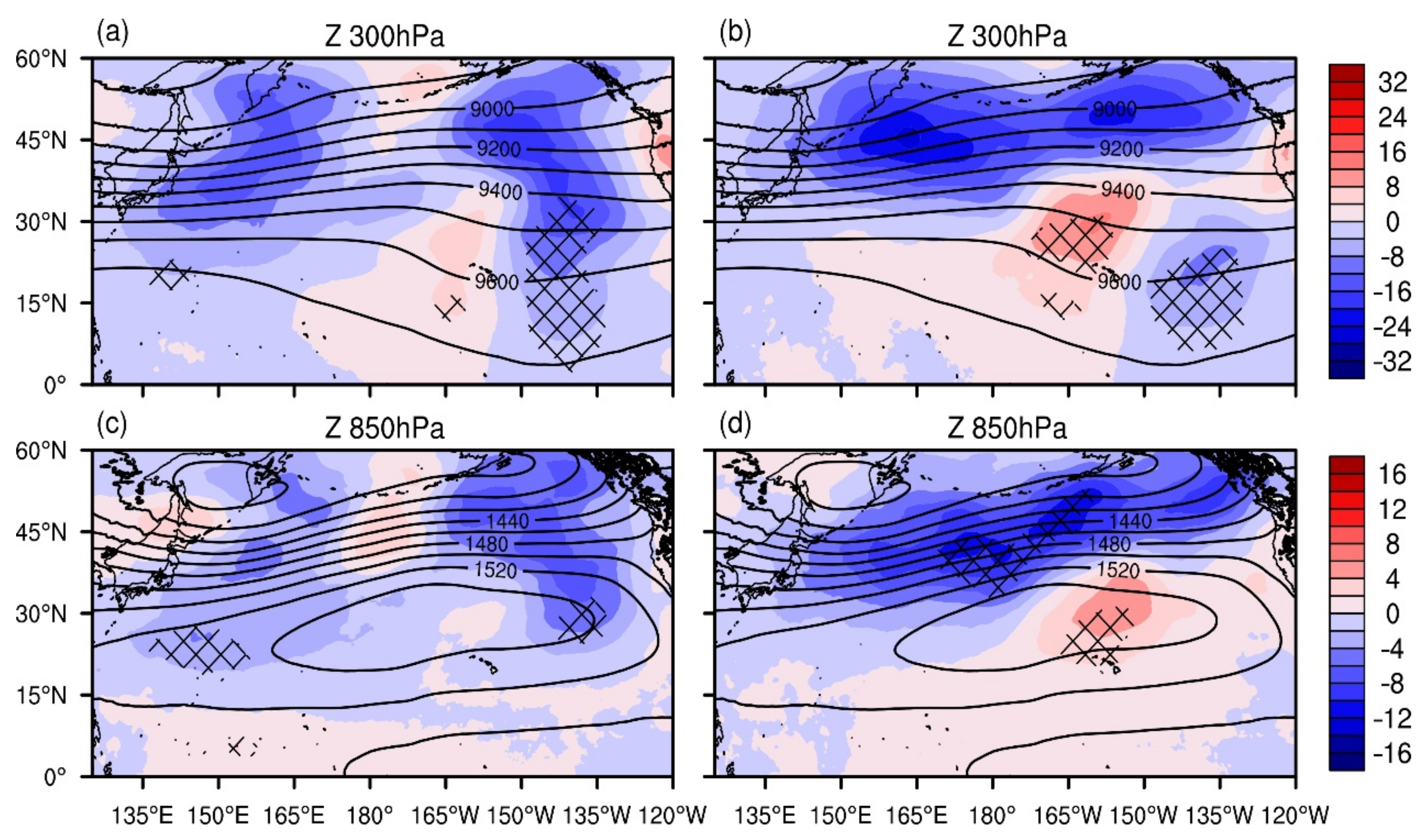
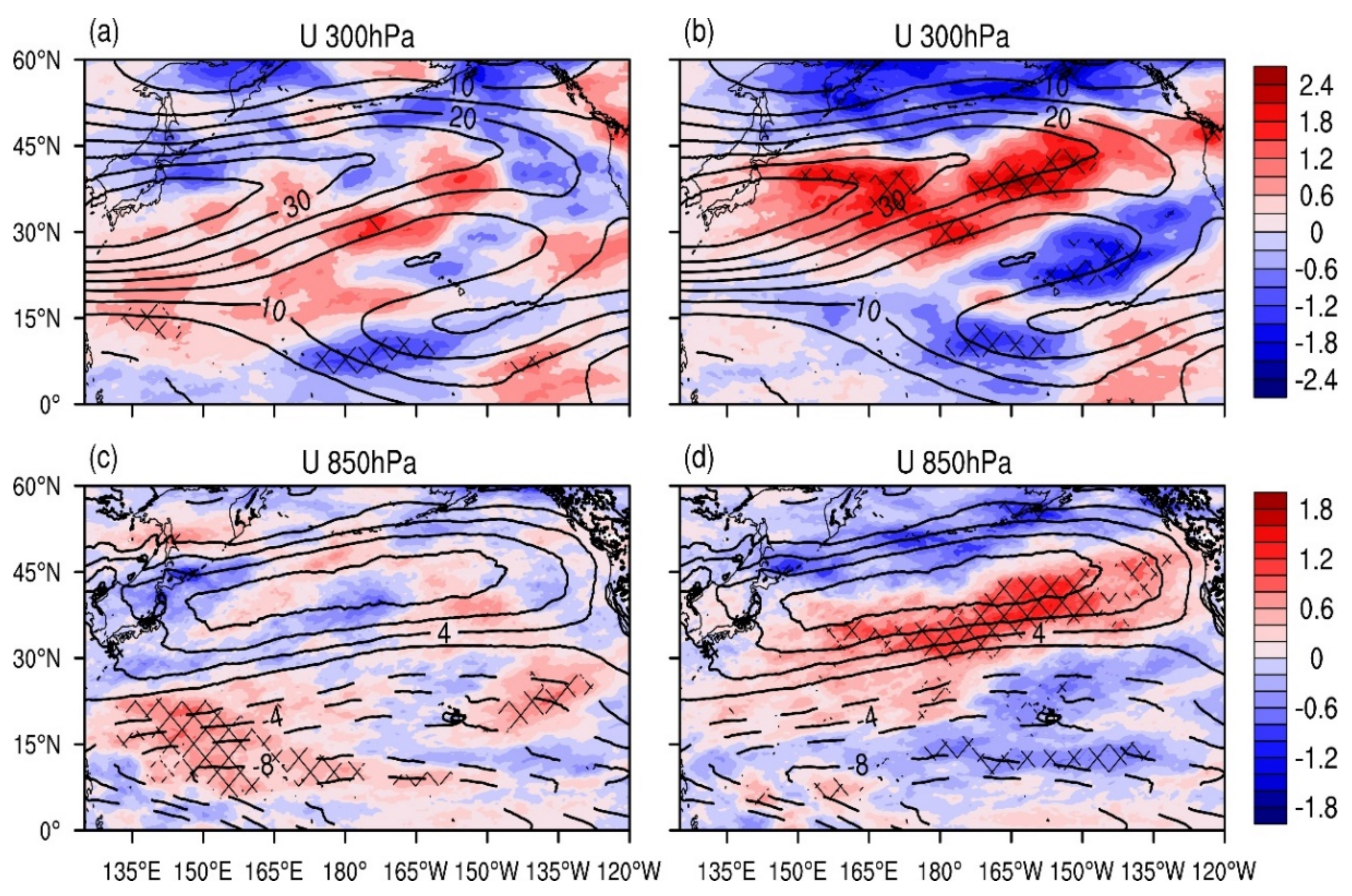
3.3. Impacts of OEs in the Northern and Southern NPac

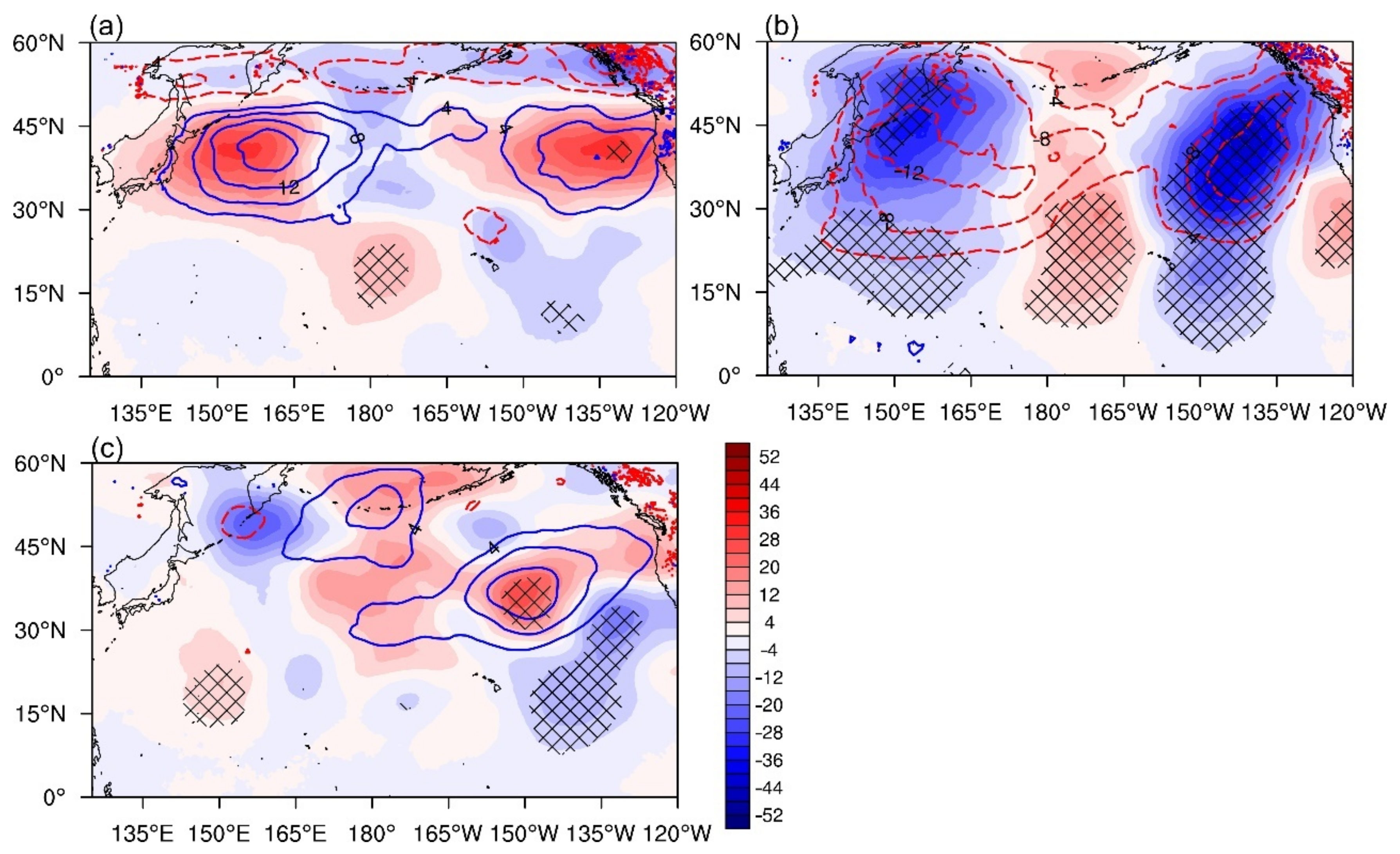
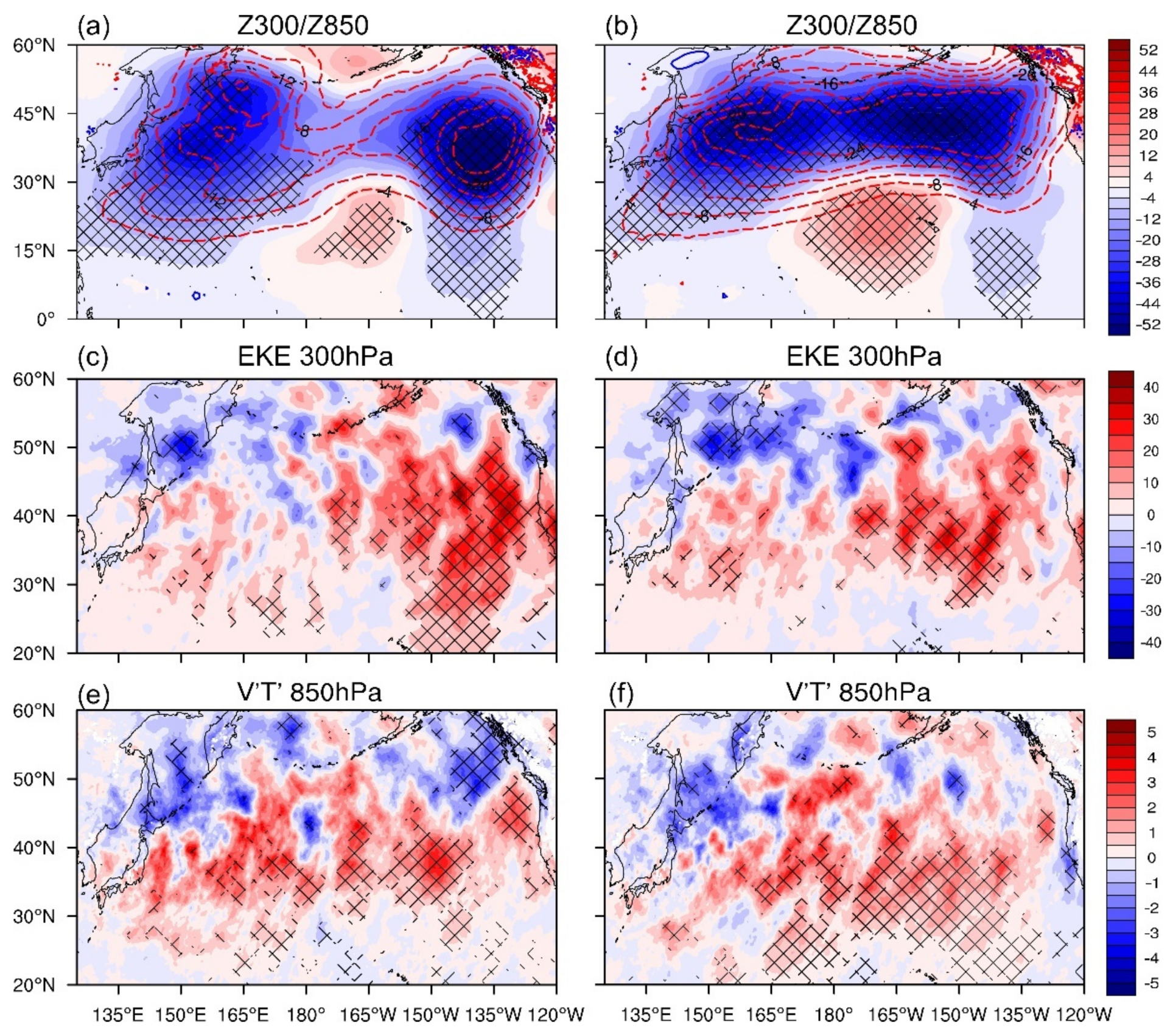
3.3.1. Atmospheric Circulations
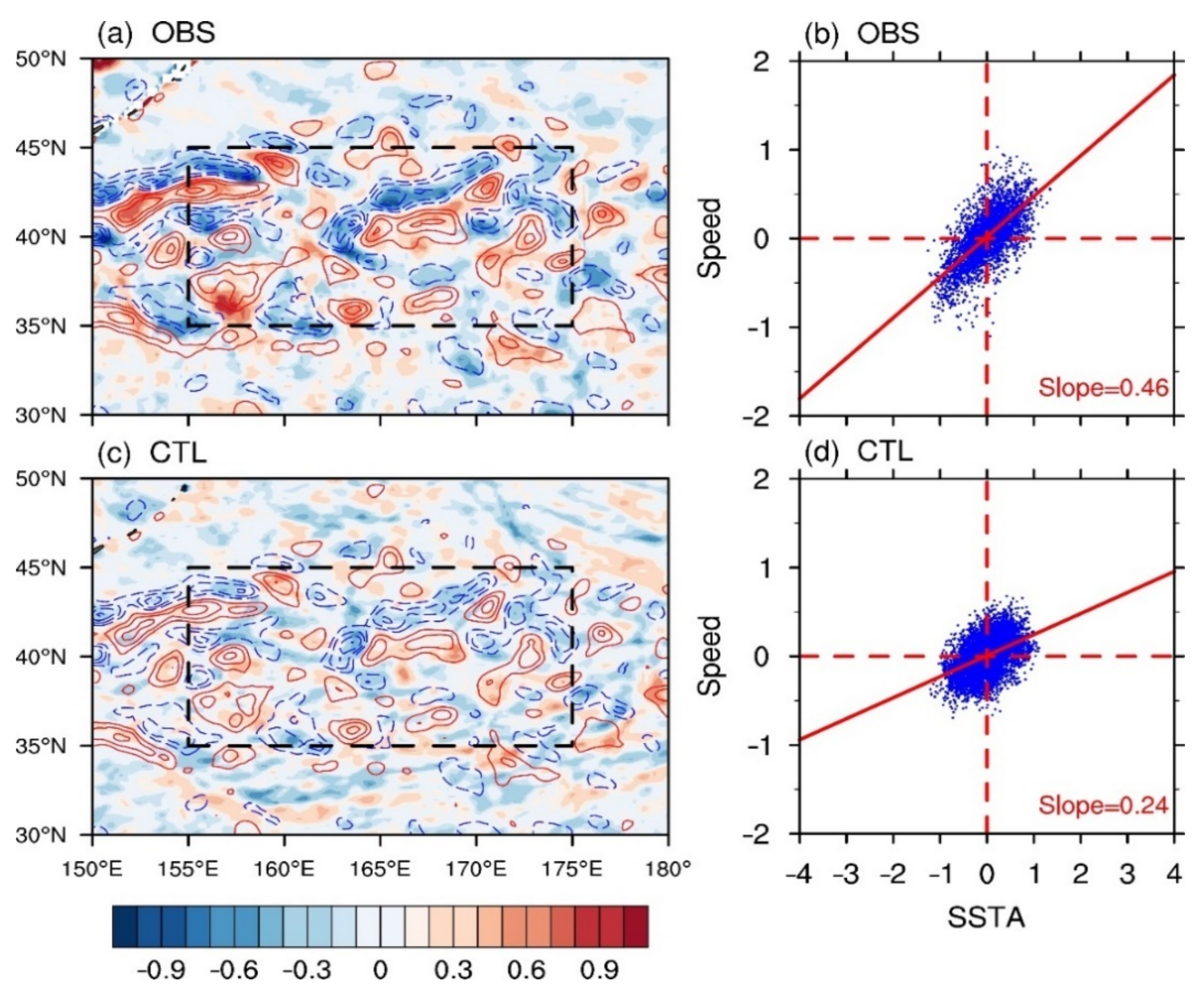
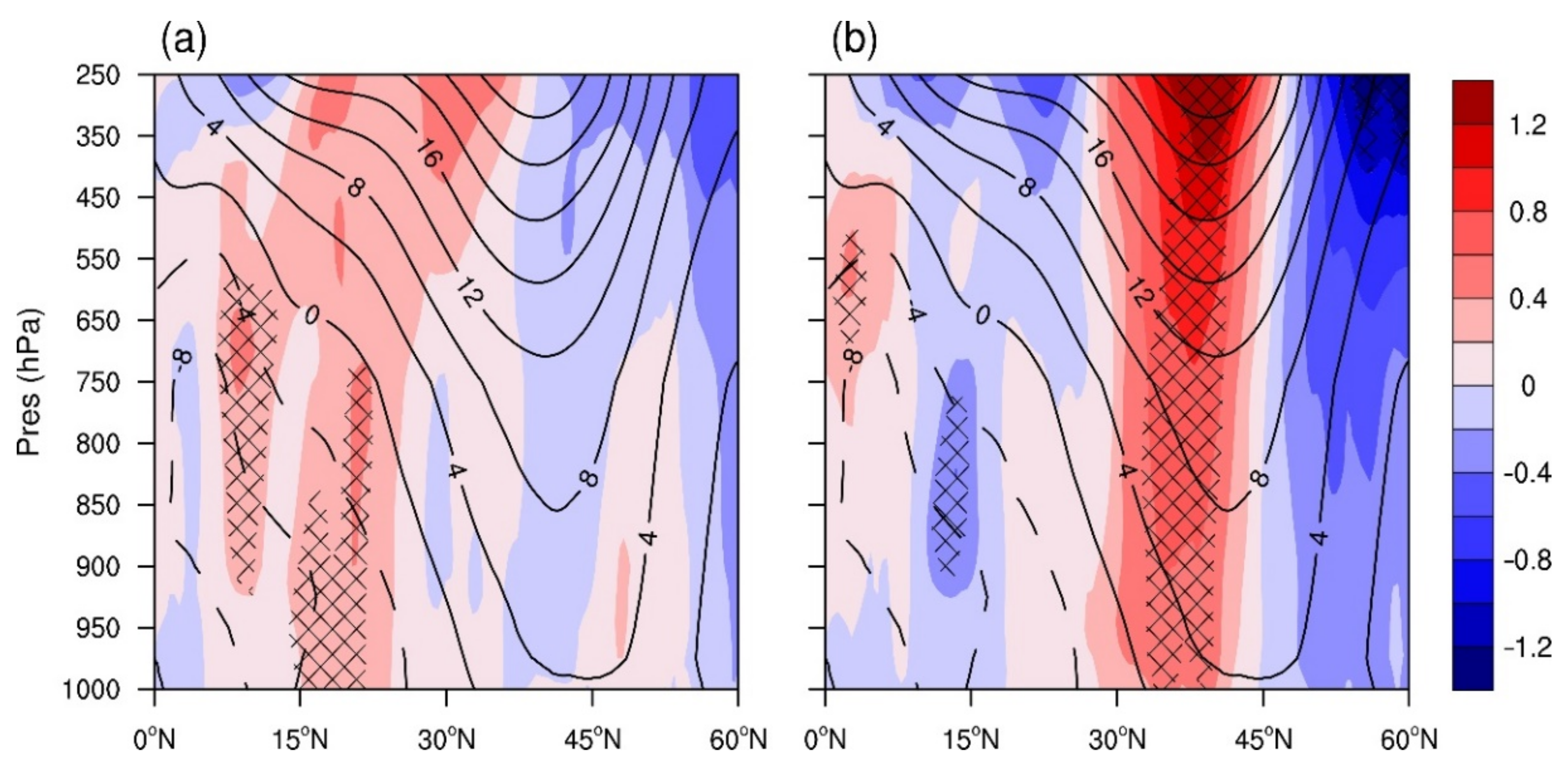
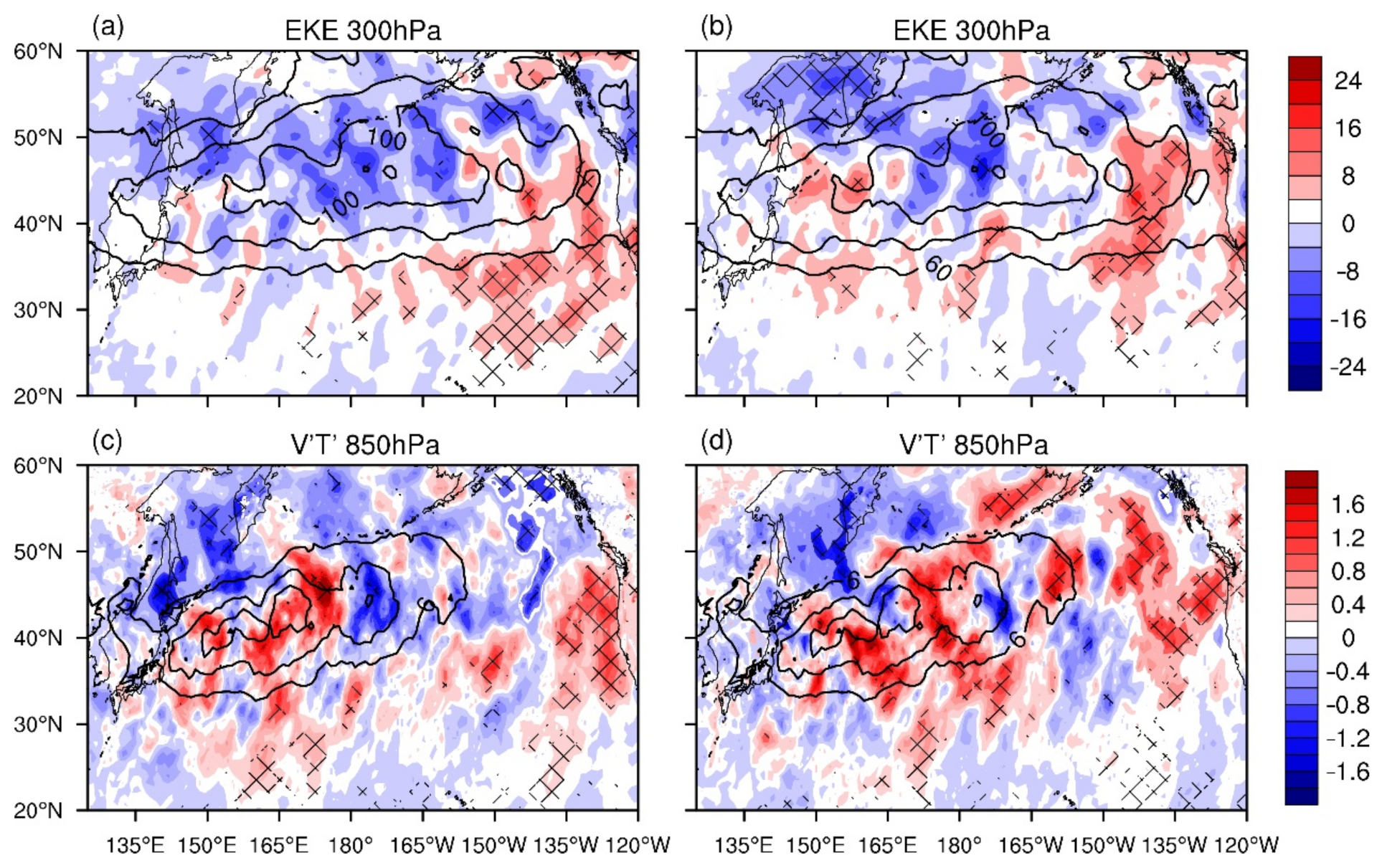
The OEs in different basins have different impacts on the overlying atmosphere [34]. Therefore, it is necessary to examine the effects of OEs in the northern and southern NPac on the atmosphere above. Figure 6 shows the differences of the upper- and lower-level GPH of SmthSST from EddySSTA + N25N and EddySSTA + S25N, respectively. When only OEs in the northern NPac are considered, the forced GPH anomalies at 300 hPa display a slightly different pattern in the NPac’s mid-to-high latitudes compared to Figure 5a, but still with two strong negative centers to the east of Japan and Alaska, respectively; this would deepen the troughs over these two regions (Figure 6a). Similar GPH anomalies are seen at 850 hPa, indicative of equivalent barotropic atmospheric responses. In addition, remarkable negative GPH anomalies appear on both the west and east sides of the PSH, suggesting that the northern NPac OEs can shrink the subtropical high (Figure 6c).
In contrast, the southern NPac OEs cause different GPH responses. A zonal band of negative GPH anomalies dominates the high latitudes at 300 hPa, extending eastward from East Japan to the Gulf of Alaska (Figure 6b). Interestingly, marked positive GPH anomalies appear in the central subtropical NPac, indicating that the southern NPac OEs act to intensify the ridge of the subtropical high, and this ridge-trough pattern is shifted eastward relative to Figure 5a. OE-induced GPH anomalies in the lower level are similar to those in the upper level, but with an obvious GPH decrease to the north of the PSH (Figure 6d), suggesting that the southern NPac OEs are conducive to the southward displacement of the lower-level PSH.
In addition, the northern NPac OEs can influence the zonal winds at both the upper and lower levels (Figure 7a,c), but significant positive anomalies are mainly confined to the tropics. The positive zonal wind anomalies at 850 hPa appear to oppose the prevailing trade wind, and thus act to reduce the northeasterly trade wind. In contrast, the southern NPac OEs can cause much larger zonal wind anomalies in the upper level, shown as enhanced westerly winds over the NPac between 30° N and 45° N and weakened westerly winds north of ~45° N (Figure 7b); a similar pattern can also be seen in the lower level (Figure 7d). This indicates that the southern NPac OEs can strengthen the upper-level westerly jet stream and shift the lower-level westerly winds southward. To confirm the above results, Figure 8 shows vertical cross sections of zonal wind changes induced by the OEs in the two NPac regions. As for the northern NPac OEs (Figure 8a), enhanced zonal winds mainly appear to the south of 20° N in the lower troposphere, weakening the lower-level trade wind over the tropical Pacific. However, the southern NPac OEs can significantly increase zonal winds over the latitude band of 30–45° N, and such positive anomalies appear to tilt northward and increase with height (Figure 8b), resulting in an accelerated westerly jet stream in the upper level and southward-shifted westerly winds in the lower level, as mentioned earlier.
The largest GPH anomalies from these three sets of experiments are mainly located in mid-to-high latitudes (Figure 5a and Figure 6a,b). We further found that these responses exhibit some sub-seasonal uncertainties in springtime, which may largely affect the significance of MAM-mean responses. Figure 9 shows the composite 850-hPa and 300-hPa GPH differences between the EddySSTA and SmthSST runs from March to May. It can be seen that April OEs can cause significant negative GPH anomalies at both 850 hPa and 300 hPa to the east of Japan and to the west coast of North America, indicative of equivalent barotropic atmospheric responses (Figure 9b). However, such GPH anomalies are partly offset by some positive GPH anomalies in the mid-to-high latitudes in March (Figure 9a) and May (Figure 9c). Meanwhile, some positive and negative GPH anomalies exist in subtropical central and eastern NPac from March to May, giving rise to obvious MAM-mean GPH anomalies in this region (Figure 5a). Sub-seasonal GPH differences also appear in EddySSTA + N25N and EddySSTA + S25N runs, but with those in April still dominating the MAM-mean responses (figure not shown).
Overall, the northern and southern NPac OEs can induce different barotropic atmospheric responses. However, the former tend to induce a wave-like GPH anomaly pattern north of 30° N, while the latter mainly induces zonally uniform GPH anomalies in the high latitudes, with larger and more significant zonal wind responses. Compared to the whole NPac OEs shown earlier (Figure 5), the northern and southern NPac OEs can independently cause much stronger atmospheric responses; specifically, the wave-like GPH anomaly pattern over the NPac’s high latitudes (north of 45° N; Figure 5a,b) mainly arises from the effects of the northern OEs (Figure 6a,c). In addition, the OEs over both NPac regions can contribute to the atmospheric circulation responses in the low latitudes, which enhances the upper-level ridge (trough) in the central (eastern) subtropical NPac (Figure 5a and Figure 6a,b) and weakens the zonal winds to the south of 15° N (Figure 5c and Figure 7a,b).

3.3.2. Storm Track

Figure 10 shows the MAM-mean differences of the upper- and lower-level storm track of SmthSST from EddySSTA + N25N and EddySSTA + S25N, respectively. For the northern NPac OEs (Figure 10c), positive poleward heat flux ( v T ) anomalies mainly appear near the core of the lower-level storm track along the KE, with obvious positive differences downstream in the eastern NPac between 35° N and 45° N. This indicates that the northern NPac OEs can enhance the storm track in these regions. Similar v T anomalies can also be induced by the southern NPac OEs, but these anomalies are slightly northward-shifted downstream in the west coast of North America (Figure 10d).
The OEs over the two NPac regions can also impact the upper-level storm track to some extent. The northern OEs could decrease EKE in the atmosphere mainly near the core of the upper-level storm track over the NPac’s mid-latitudes, and the downstream region of the eastern NPac also sees some negative EKE anomalies north of 45° N and positive anomalies to the south. This means that the NPac’s spring storm track in the upper level is mainly weakened by the northern OEs with a southward shift in the downstream region (Figure 10a). Similarly, the southern OEs cause negative EKE anomalies over most areas of the storm track, but these anomalies are only confined to the west of the International Dateline, while some positive EKE anomalies appear in the downstream region (Figure 10b).
Generally, the lower-level storm track largely depends on the meridional gradient of the lower-level atmospheric temperature or SST, and thus the atmospheric baroclinicity [15,53,54]. However, because of their spatial scales, much smaller than the atmospheric Rossby deformation radius, mesoscale OEs may exert limited impacts on the lower-level atmospheric baroclinicity. Deremble et al. [63] suggested that OEs could lead to an enhanced diabatic heating and thus strengthen the lower-level storm track via enhancing surface evaporation and moistening the boundary layer. Figure 11 shows the differences of water vapor, vertically averaged from 1000 to 850 hPa, induced by OEs. The northern NPac OEs can increase water vapor near the center of the lower-level storm track from 150° E to 180° (green solid line in Figure 11a). In addition, water vapor also increased over the downstream NPac east of 150° W, which is consistent with the strengthened storm track in this region, shown in Figure 10c. However, water vapor anomalies induced by the southern NPac OEs at the center of lower-level storm track are relatively weak (Figure 11b), and larger positive anomalies are mainly found downstream of the eastern NPac, corresponding to the enhanced lower-level storm track off the west coast of North America (Figure 10d). The OE-induced diabatic heating also increased in the downstream west coast of North America (figure not shown).

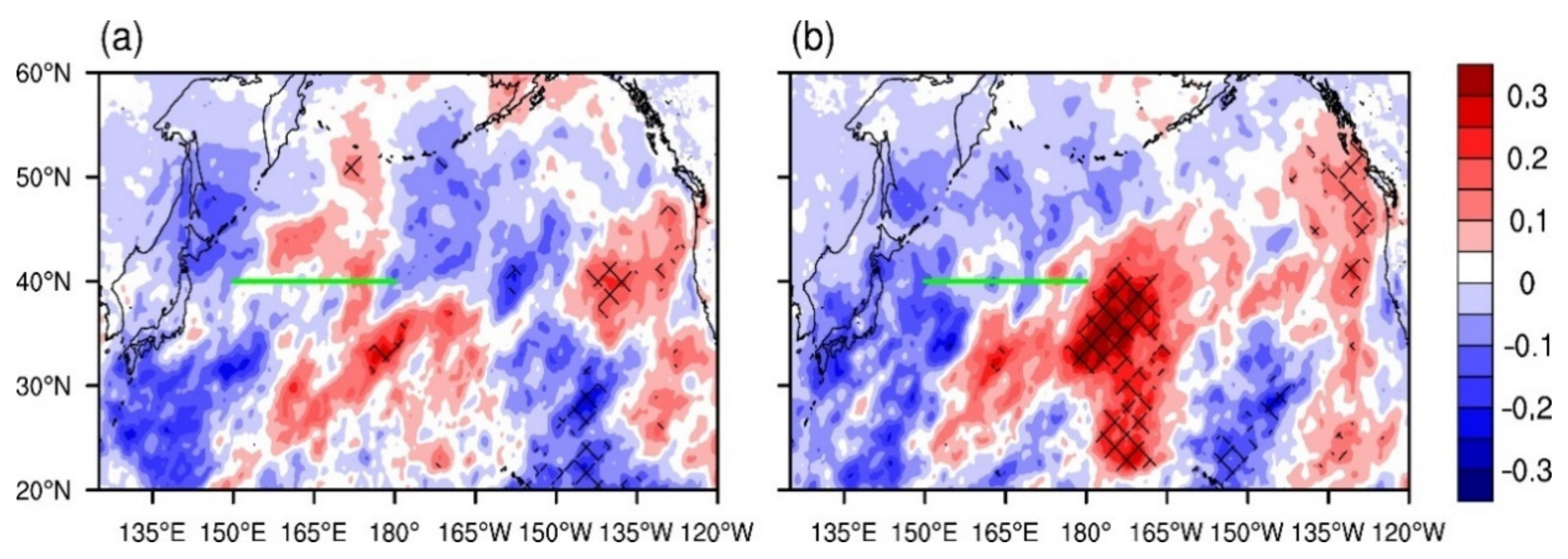
3.4. Sub-Seasonal Varitions

Compared with the atmospheric responses to OEs in EddySSTA runs, the northern and southern NPac OEs have more evident impacts than that of whole NPac OEs. However, these atmospheric responses in MAM exhibit sub-seasonal variations with the dominant response in April. Figure 12 shows the mean differences in April of the upper- and lower-level GPH and the storm track of SmthSST from EddySSTA + N25N and EddySSTA + S25N, respectively. The northern NPac OEs can induce marked negative GPH anomalies at both 850 hPa and 300 hPa near the western and eastern coasts (Figure 12a), indicative of equivalent barotropic atmospheric responses. For the southern NPac OEs, the OEs lead to negative GPH anomalies at 300 hPa in the mid-to-high latitudes, extending eastward from East Japan to the Gulf of Alaska. Meanwhile, marked positive GPH anomalies appear in the central NPac (~30° N), indicating that the southern NPac OEs mainly act to intensify the subtropical high. OE-induced GPH anomalies at the lower level (Figure 12b) are also similar to those in the upper level.
When only the northern NPac OEs are included in the model, positive poleward heat flux ( v T ) anomalies at the lower level mainly appear along the KE, and with significantly positive differences downstream in the eastern NPac between 30° N and 45° N. This indicates that the northern NPac OEs can enhance the lower-level storm activities in these regions during April (Figure 12e). Similar v T anomalies can also be induced by the southern NPac OEs, but the anomalies are mainly confined, in the central NPac, to the south of 40° N (Figure 12f).
The northern NPac OEs induce significantly positive EKE anomalies over the downstream eastern NPac (Figure 12c) and thus strengthen the upper-level storm activities. Meanwhile, the southern OEs cause negative EKE anomalies to the west of the International Dateline north of 45° N, and the positive EKE anomalies mainly appear in the downstream region (Figure 12d).
Comparing the lower-level storm activity responses in April (Figure 12e,f) with that in MAM (Figure 10c,d), it is found that the southern NPac OEs do not exert evident impacts on the storm track over the west coast of North America on the seasonal mean time scale. On the sub-seasonal time scale, the southern NPac OEs in May (figure not shown) can still cause significant GPH and zonal wind anomalies, contributing to an eastward shift of the ridge-trough pattern south of 30° N (Figure 6b) and a northward shift of the zonal wind anomalies in MAM compared to that in April (figure not shown). Here, the southern NPac OEs in May can strengthen the storm activities in western NPac around 40° N. In the downstream west coast of North America, the southern NPac OEs significantly strengthen the storm activities to the north of 40° N, weakening the storm activities to the south of 40° N. As a result, the southern NPac OEs can cause a northward shift of the lower-level MAM-mean storm track responses in the downstream eastern NPac (Figure 10d) compared to that induced by northern NPac OEs (Figure 10c).

4. Conclusions and Discussion

Using the OE detection dataset and a high-resolution WRF model, we mainly investigated the climatic effects of mesoscale OEs in the NPac in spring (MAM). We also compared different effects of OEs in the northern NPac associated with the KE and those in the southern part related to the subtropical countercurrent. Our main conclusions are as follows:
(1) The mesoscale OEs in the whole NPac have effects on the overlying atmospheric circulations and storm track to some extent. OEs can significantly strengthen the upper-level ridge (trough) in the central (eastern) subtropical NPac, together with weakened (strengthened) westerly winds to the south. At the lower level, there are negative GPH anomalies to the west of the PSH, which weakens the easterly trade wind in the low latitudes. In mid-to-high latitudes, OEs can deepen the two troughs in Okhotsk and Alaska. In general, mesoscale OEs act to weaken the upper-level storm track and strengthen the lower-level storm activities in the NPac.
(2) The northern and southern NPac OEs have more evident impacts than that of whole NPac OEs and have canceling impacts on the atmosphere to some extent. The atmospheric responses over the mid-to-high latitudes are dominated by the northern OEs, but the responses over the low latitudes are affected by both northern and southern OEs. Despite different influences on atmospheric circulations, the southern and northern NPac OEs have similar local impacts on the lower-level storm track in the KE and significant remote effects on storm activities over the Northeast Pacific off the west coast of North America, probably through the increasing water vapor content in the marine atmospheric boundary layer.
(3) On the sub-seasonal timescale, atmospheric responses induced by the whole, northern, and southern NPac OEs all exhibit some intra-seasonal differences in springtime with the most dominant responses in April, which largely determine the overall responses in MAM.
We also found that the OEs in the southern NPac can cause much stronger atmospheric responses despite their smaller amount and weaker magnitude. This result is similar to that of Huang et al. [54], which showed that the climatic effects of the wintertime double-oceanic-front structure in the NPac are characterized by weaker atmospheric responses to the northern ocean fronts. As noted previously [8,9,10,11,12,14,54], the turbulent heat fluxes may also play crucial roles in mesoscale air-sea interactions. Thus, we further analyzed the composite differences of spring turbulent heat fluxes between EddySSTA + N25N and SmthSST, and EddySSTA + S25N and SmthSST runs. OEs have effects on turbulent heat fluxes, but these effects could not explain the composite differences in climatic effects of northern and southern eddy SSTAs, which may largely depend on the internal adjustment of the atmosphere or other factors. Using an idealized global climate model (GCM) with SSTAs embedded in different ocean basins, Thomson and Vallis [64] suggested that many of the mid-latitude SSTAs were not able to cause large atmospheric responses, as they are highly sensitive to the background state, while the responses to tropical SSTAs were much more robust.
To further confirm our results and compare the effects of OEs with those of other mesoscale processes, several additional sensitivity simulations were carried out. They are driven by doubled eddy-related SSTAs, a smooth SST to the north of 25° N, or a smooth SST to the south of 25° N. In the eddy intensity-doubling cases, the effects on the atmosphere are robust and similar to the original results, but with a larger and more significant magnitude. For the climatic effects of total SSTAs, we find that the northern and southern SSTAs have similar effects, but the former have stronger effects. In addition to causing a westward displacement of the upper-level zonal wind, a northward shift of the downstream storm activities also appears in the downstream eastern NPac, which is consistent with the result of Ma et al. [29,30]. However, comparing these effects with those of the northern and southern OEs, we can see that the southern OEs have more prominent effects than the northern OEs; and the springtime OEs play an opposite role in mesoscale SSTAs, which could result in an eastward displacement of the upper-level zonal wind and a southward shift of the downstream storm activities off the west coast of North America. Please note also the exit of a large amount of OEs near the KE and subtropical counter current, especially over the eastern part of the NPac. Accordingly, we also performed two numerical experiments by adding OEs only in the western or eastern NPac, respectively, and found that the climatic effects of the western NPac OEs are stronger than those of the eastern NPac OEs at seasonal timescales.
Although our results show clear climatic effects of mesoscale OEs over the whole, northern, and southern NPac, some limitations exist. First, a uniform scale of about 500 km is used to define the SSTAs associated with mesoscale OEs, that have typical scales ranging from 100 to 500 km. Therefore, more sensitivity experiments using different scales are needed in the future. Second, the coupling strength of surface wind speed-SST in CTL is weaker than that in the observations, which may weaken the climatic effects of OEs. Third, our WRF results can only show parts of the complex coupled ocean-atmosphere interactions in the real world, as we used the prescribed ocean boundary condition in this study. Thus, it is necessary to use a coupled ocean-atmosphere model to investigate the climatic effects of OEs and shed light on their seasonal variation.

Author Contributions

Conceptualization, H.X.; methodology, H.X.; software, Z.C.; validation, H.X., J.M. and J.D.; formal analysis, Z.C.; investigation, Z.C.; resources, H.X.; data curation, Z.C.; writing—original draft preparation, Z.C.; writing—review and editing, H.X., J.M. and J.D.; visualization, Z.C.; supervision, H.X.; project administration, H.X.; funding acquisition, H.X. All authors have read and agreed to the published version of the manuscript.

Funding

This work is jointly supported by the National Natural Science Foundation of China (41975106, 41805051, and 41705054), the National Key Research and Development Program of China (2017YFA0604100), and the Startup Foundation for Introducing Talent of NUIST (2017r057 and 2016r051).

Data Availability Statement

Not applicable.

Acknowledgments

The numerical calculations in this paper have been done on the supercomputing system in the Supercomputing Center of NUIST.

Conflicts of Interest

The authors declare no conflict of interest.

References

  1. Kushnir, Y.; Robinson, W.A.; Blade, I.; Hall, N.M.J.; Peng, S.; Sutton, R. Atmospheric GCM response to extratropical SST anomalies: Synthesis and Evaluation. J. Clim. 2002, 15, 2233–2256. [Google Scholar] [CrossRef] [Green Version]
  2. Wentz, F.J.; Schabel, M.C. Precise climate monitoring using complementary satellite data sets. Nature 2000, 403, 414–416. [Google Scholar] [CrossRef] [PubMed]
  3. Chelton, D.B.; Schlax, M.G.; Freilich, M.H.; Milliff, R.F. Satellite measurements reveal persistent small-scale features in ocean winds. Science 2004, 303, 978–983. [Google Scholar] [CrossRef] [PubMed] [Green Version]
  4. Xie, S.P. Satellite observations of cool ocean-atmosphere interaction. Bull. Am. Meteorol. Soc. 2004, 85, 195–208. [Google Scholar] [CrossRef] [Green Version]
  5. Chelton, D.B.; Wentz, F.J. Global microwave satellite observations of sea surface temperature for numerical weather prediction and climate research. Bull. Am. Meteorol. Soc. 2005, 86, 1097–1115. [Google Scholar] [CrossRef] [Green Version]
  6. Chelton, D.B.; Xie, S.P. Coupled ocean-atmosphere interaction at oceanic mesoscale. Oceanography 2010, 23, 52–69. [Google Scholar] [CrossRef]
  7. Byrne, D.; Papritz, L.; Frenger, I.; Munnich, M.; Gruber, N. Atmospheric response to mesoscale sea surface temperature anomalies: Assessment of mechanisms and coupling strength in a high-resolution coupled model over the South Atlantic. J. Atmos. Sci. 2015, 72, 1872–1890. [Google Scholar] [CrossRef] [Green Version]
  8. Minobe, S.; Kuwano-Yoshida, A.; Komori, N.; Xie, S.P.; Small, R.J. Influence of the Gulf Stream on the troposphere. Nature 2008, 452, 206–209. [Google Scholar] [CrossRef] [PubMed]
  9. Small, R.J.; Deszoeke, S.P.; Xie, S.P.; O’Neull, L.; Seo, H.; Song, Q.; Cornillon, P.; Spall, M.; Minobe, S. Air-sea interaction over ocean fronts and eddies. Dyn. Atmos. Ocean. 2008, 45, 274–319. [Google Scholar] [CrossRef]
  10. Iizuka, S. Simulations of wintertime precipitation in the vicinity of Japan: Sensitivity to fine-scale distributions of sea surface temperature. J. Geophys. Res. Atmos. 2010, 115. [Google Scholar] [CrossRef] [Green Version]
  11. Kuwano-Yoshida, A.; Minobe, S.; Xie, S.P. Precipitation response to the Gulf Stream in an atmospheric GCM. J. Clim. 2010, 23, 3676–3698. [Google Scholar] [CrossRef]
  12. O’neill, L.W.; Chelton, D.B.; Esbensen, S.K. Covariability of surface wind and stress responses to sea surface temperature fronts. J. Clim. 2012, 25, 5916–5942. [Google Scholar] [CrossRef] [Green Version]
  13. Saravanan, R.; Chang, P. Midlatitude mesoscale ocean-atmosphere interaction and its relevance to S2S prediction. In Sub-Seasonal to Seasonal Prediction; Elsevier: Amsterdam, The Netherlands, 2019; pp. 183–200. [Google Scholar] [CrossRef]
  14. Nakamura, H.; Sampe, T.; Tanimoto, Y.; Shimpo, A. Observed associations among storm tracks, jet streams and midlatitude oceanic fronts. In Earth’s Climate: The Ocean-Atmosphere Interaction; Geophysical Monograph Series; American Geophysical Union: Washington, DC, USA, 2004; Volume 147, pp. 329–345. [Google Scholar] [CrossRef] [Green Version]
  15. Taguchi, B.; Nakamura, H.; Nonaka, M.; Xie, S.P. Influences of the Kuroshio/Oyashio Extensions on air-sea heat exchanges and storm-track activity as revealed in regional atmospheric model simulations for the 2003/04 cold season. J. Clim. 2009, 22, 6536–6560. [Google Scholar] [CrossRef] [Green Version]
  16. Small, R.J.; Tomas, R.A.; Bryan, F.O. Storm track response to ocean fronts in a global high-resolution climate model. Clim. Dyn. 2014, 43, 805–828. [Google Scholar] [CrossRef]
  17. Piazza, M.; Terray, L.; Boe, J.; Maisonnave, E.; Sanchez-Gomez, E. Influence of small-scale North Atlantic sea surface temperature patterns on the marine boundary layer and free troposphere: A study using the atmospheric ARPEGE model. Clim. Dyn. 2016, 46, 1699–1717. [Google Scholar] [CrossRef]
  18. Bourras, D.; Reverdin, G.; Giordani, H.; Caniaux, G. Response of the atmospheric boundary layer to a mesoscale oceanic eddy in the northeast Atlantic. J. Geophys. Res. Atmos. 2004, 109, 1–19. [Google Scholar] [CrossRef]
  19. Chou, C.H.; Liu, Q. Eddy effects on sea surface temperature and sea surface wind in the continental slope region of the northern South China Sea. Geophys. Res. Lett. 2012, 39, L02601. [Google Scholar] [CrossRef]
  20. Lambaerts, J.; Lapeyre, G.; Plougonven, R.; Klen, P. Atmospheric response to sea surface temperature mesoscale structures. J. Geophys. Res. Atmos. 2013, 118, 9611–9621. [Google Scholar] [CrossRef] [Green Version]
  21. Li, W.B.; Liu, H.Y.; Fang, R. Review of the atmospheric response to the ocean mesoscale eddies. Adv. Earth Sci. 2017, 32, 1039–1049. [Google Scholar] [CrossRef]
  22. Frenger, I.; Gruber, N.; Knutti, R.; Munnich, M. Imprint of southern ocean eddies on winds, clouds and rainfall. Nat. Geosci. 2013, 6, 608–612. [Google Scholar] [CrossRef]
  23. Rouault, M.; Verley, P.; Backeberg, B. Wind increase above warm Agulhas Current eddies. Ocean Sci. Discuss. 2014, 11, 2367–2389. [Google Scholar] [CrossRef] [Green Version]
  24. Gaube, P.; Chelton, D.B.; Samelson, R.M.; Schlax, M.G.; O’Neill, L.W. Satellite observations of mesoscale eddy-induced ekman pumping. J. Phys. Oceanogr 2015, 45, 104–132. [Google Scholar] [CrossRef]
  25. Shan, H.; Dong, C. Atmospheric responses to oceanic mesoscale eddies based on an idealized model. Int. J. Climatol. 2019, 39, 1665–1683. [Google Scholar] [CrossRef]
  26. Ma, J.; Xu, H.; Dong, C.; Lin, P.; Liu, Y. Atmospheric responses to oceanic eddies in the Kuroshio Extension region. J. Geophys. Res. Atmos. 2015, 120, 6313–6330. [Google Scholar] [CrossRef]
  27. Ma, J.; Xu, H.; Dong, C. Seasonal variations in atmospheric responses to oceanic eddies in the Kuroshio Extension. Tellus A Dyn. Meteorol. Oceanogr. 2016, 68, 31563. [Google Scholar] [CrossRef] [Green Version]
  28. Perlin, N.; De Szoeke, S.P.; Chelton, D.B.; Samelson, R.M.; Skyllingstad, E.D.; O’Neill, L.W. Modeling the atmospheric boundary layer wind response layer wind response to mesoscale sea surface temperature perturbations. Mon. Weather Rev. 2014, 142, 4284–4307. [Google Scholar] [CrossRef] [Green Version]
  29. Ma, X.; Chang, P.; Saravanan, R.; Montuoro, R.; Hsieh, J.; Wu, D.; Lin, X.; Wu, L.; Jing, Z. Distant influence of Kuroshio eddies on North Pacific weather patterns. Sci. Rep. 2015, 5, 17785. [Google Scholar] [CrossRef] [Green Version]
  30. Ma, X.; Chang, P.; Saravanan, R.; Monturo, R.; Nakamura, H.; Wu, D.; Lin, X.; Wu, L. Importance of resolving Kuroshio front and eddy influence in simulating the North Pacific storm track. J. Clim. 2017, 30, 1861–1880. [Google Scholar] [CrossRef]
  31. Foussard, A.; Lapeyre, G.; Plougonven, R. Storm track response to oceanic eddies in idealized atmospheric simulations. J. Clim. 2019, 32, 445–463. [Google Scholar] [CrossRef]
  32. Liu, Y.; Dong, C.; Guan, Y.; Chen, D.; McWilliams, J.; Nencioli, F. Eddy analysis in the subtropical zonal band of the North Pacific Ocean. Deep Sea Res. Part I Oceanogr. Res. Pap. 2012, 68, 54–67. [Google Scholar] [CrossRef]
  33. Ji, J.; Dong, C.; Zhang, B.; Liu, Y.; Zou, B.; King, G.P.; Xu, G.; Chen, D. Oceanic eddy characteristics and generation mechanisms in the Kuroshio Extension region. J. Geophys. Res. Ocean. 2018, 123, 8548–8567. [Google Scholar] [CrossRef]
  34. Ji, J.; Ma, J.; Dong, C.; Chiang, J.C.H.; Chen, D. Regional dependence of atmospheric responses to oceanic eddies in the North Pacific ocean. Remote Sens. 2020, 12, 1161. [Google Scholar] [CrossRef] [Green Version]
  35. Putrasahan, D.A.; Miller, A.J.; Seo, H. Isolating mesoscale coupled ocean–atmosphere interactions in the kuroshio extension region. Dyn. Atmos. Ocean. 2013, 63, 60–78. [Google Scholar] [CrossRef]
  36. Seo, H.; Miller, A.J.; Norris, J.R. Eddy–wind interaction in the California Current System: Dynamics and impacts. J. Phys. Oceanogr. 2016, 46, 439–459. [Google Scholar] [CrossRef]
  37. Jia, Y.; Chang, P.; Szunyogh, I.; Saravanan, R.; Bacmeister, J.T. A modeling strategy for the investigation of the effect of mesoscale SST variability on atmospheric dynamics. Geophys. Res. Lett. 2019, 46, 3982–3989. [Google Scholar] [CrossRef]
  38. Kobashi, F.; Kawamura, H. Seasonal variation and instability nature of the North Pacific Subtropical Countercurrent and the Hawaiian Lee Countercurrent. J. Geophys. Res. Ocean. 2002, 107, 6-1–6-18. [Google Scholar] [CrossRef]
  39. Qiu, B.; Chen, S. Interannual variability of the North Pacific subtropical countercurrent and its associated mesoscale eddy field. J. Phys. Oceanogr. 2010, 40, 215–225. [Google Scholar] [CrossRef]
  40. Reynolds, R.W.; Smith, T.M.; Liu, C.; Chelton, D.B.; Casey, K.S.; Schlax, M.G. Daily high-resolution-blended analyses for sea surface temperature. J. Clim. 2007, 20, 5473–5496. [Google Scholar] [CrossRef]
  41. Liu, T.W.; Xie, X.; Polito, P.S.; Xie, S.P.; Hashizume, H. Atmospheric manifestation of tropical instability wave observed by QuikSCAT and tropical rain measuring mission. Geophys. Res. Lett. 2000, 27, 2545–2548. [Google Scholar] [CrossRef] [Green Version]
  42. Saha, S.; Moorthi, S.; Pan, H.L.; Wu, X.; Wang, J.; Nadiga, S.; Tripp, P.; Kistler, R.; Woollen, J.; Behringer, D. The NCEP climate forecast system reanalysis. Bull. Am. Meteorol. Soc. 2010, 91, 1015–1058. [Google Scholar] [CrossRef]
  43. Liu, J.W.; Zhang, S.P.; Xie, S.P. Two types of surface wind responses to the East China Sea Kuroshio front. J. Clim. 2013, 26, 8616–8627. [Google Scholar] [CrossRef]
  44. Chelton, D.B.; Schlax, M.G.; Samelson, R.M. Global observations of nonlinear mesoscale eddies. Prog. Oceanogr. 2011, 91, 167–216. [Google Scholar] [CrossRef]
  45. Williams, S.; Petersen, M.; Bremer, P.T.; Hecht, M.; Pascucci, V.; Ahrens, J.; Hlawitschka, M.; Hamann, B. Adaptive extraction and quantification of geophysical vortices. IEEE Trans. Vis. Comput. Graph. 2011, 17, 2088–2095. [Google Scholar] [CrossRef] [PubMed] [Green Version]
  46. Willison, J.; Robinson, W.A.; Lackmann, G.M. The importance of resolving mesoscale latent heating in the North Atlantic storm track. J. Atmos. Sci. 2013, 70, 2234–2250. [Google Scholar] [CrossRef]
  47. Pujol, M.I.; Faugere, Y.; Taburet, G.; Dupuy, S.; Pelloquin, C.; Ablain, M.; Picot, N. DUACS DT2014: The new multi-mission altimeter dataset reprocessed over 20 years. Ocean Sci. Discuss. 2016, 12, 1067–1090. [Google Scholar] [CrossRef] [Green Version]
  48. Skamarock, W.C.; Klemp, J.B.; Dudhia, J.; Gill, D.O.; Barker, D.M.; Duda, M.G.; Huang, X.; Wang, W.; Powers, J.G. A Description of the Advanced Research WRF Version 3; NCAR Tech. Note/TN-475+ STR; University Corporation for Atmospheric Research: Boulder, CO, USA, 2008. [Google Scholar]
  49. O’neill, L.W.; Esbensen, S.K.; Thum, N.; Samelson, R.M.; Chelton, D.B. Dynamical analysis of the boundary layer and surface wind responses to mesoscale SST perturbations. J. Clim. 2010, 23, 559–581. [Google Scholar] [CrossRef] [Green Version]
  50. Zhou, G.; Latif, M.; Greatbatch, R.J.; Park, W. Atmosphereric response to the North Pacific enabled by daily sea surface temperature variability. Geophys. Res. Lett. 2015, 42, 7732–7739. [Google Scholar] [CrossRef] [Green Version]
  51. Dong, C.; Nencioli, F.; Liu, Y.; McWilliams, J.C. An automated approach to detect oceanic eddies from satellite remotely sensed sea surface temperature data. IEEE Geosci. Remote Sens. Lett. 2011, 8, 1055–1059. [Google Scholar] [CrossRef]
  52. Greene, C.A.; Thirumalai, K.; Kearney, K.A.; Delgado, J.M.; Schwanghart, W.; Wolfenbarger, N.S.; Thyng, K.M.; Gwyther, D.E.; Gardner, A.S.; Blankenship, D.D. The climate data toolbox for MATLAB. Geochem. Geophys. Geosyst. 2019, 20, 3774–3781. [Google Scholar] [CrossRef] [Green Version]
  53. Yao, Y.; Zhong, Z.; Yang, X. Numerical experiments of the storm track sensitivity to oceanic frontal strength within the Kuroshio/Oyashio Extensions. J. Geophys. Res. Atmos. 2016, 121, 2888–2900. [Google Scholar] [CrossRef]
  54. Huang, J.; Zhang, Y.; Yang, X.; Ren, X.; Hu, H. Impacts of North Pacific subtropical and subarctic oceanic frontal zones on the wintertime atmospheric large-scale circulations. J. Clim. 2020, 33, 1897–1914. [Google Scholar] [CrossRef]
  55. O’neill, L.W.; Chelton, D.B.; Esbensen, S.K. Observations of SST-induced perturbations of the wind stress field over the Southern Ocean on seasonal time scales. J. Clim. 2003, 16, 2340–2354. [Google Scholar] [CrossRef] [Green Version]
  56. Chelton, D.B.; Schlax, M.G.; Samelson, R.M. Summertime coupling between sea surface temperature and wind stress in the California Current System. J. Phys. Oceanogr. 2007, 37, 495–517. [Google Scholar] [CrossRef]
  57. Seo, H.; Murtugudde, R.; Jochum, M.; Mller, A.J. Modeling of mesoscale coupled ocean-atmosphere interaction and its feedback to ocean in the western Arabian Sea. Ocean Model. 2008, 25, 120–131. [Google Scholar] [CrossRef]
  58. Bryan, F.O.; Tomas, R.A.; Dennis, J.M.; Dudley, B.C. Frontal scale air–sea interaction in high-resolution coupled climate models. J. Clim. 2010, 23, 6277–6291. [Google Scholar] [CrossRef]
  59. Zhang, R.H. Effects of tropical instability wave (TIW)-induced surface wind feedback in the tropical Pacific Ocean. Clim. Dyn. 2014, 42, 467–485. [Google Scholar] [CrossRef]
  60. Gao, J.; Zhang, R.H.; Wang, H. Mesoscale SST perturbation-induced impacts on climatological precipitation in the Kuroshio-Oyashio extension region, as revealed by the WRF simulations. J. Oceanol. Limnol. 2019, 37, 385–397. [Google Scholar] [CrossRef]
  61. Song, Q.; Chelton, D.B.; Esbensen, S.K.; Thum, N.; O’Neill, L.W. Coupling between sea surface temperature and low-level winds in mesoscale numerical models. J. Clim. 2009, 22, 146–164. [Google Scholar] [CrossRef]
  62. Booth, J.F.; Thompson, L.A.; Patoux, J.; Kathryn, A.K.; Dickinson, S. The signature of the midlatitude tropospheric storm tracks in the surface winds. J. Clim. 2010, 23, 1160–1174. [Google Scholar] [CrossRef] [Green Version]
  63. Deremble, B.; Lapeyre, G.; Ghil, M. Atmospheric dynamics triggered by an oceanic SST front in a mosit quasigeostrophic model. J. Atmos. Sci. 2012, 69, 1617–1632. [Google Scholar] [CrossRef] [Green Version]
  64. Thomson, S.I.; Vallis, G.K. Atmospheric response to SST anomalies. Part I: Background-state dependence, teleconnections, and local effects in winter. J. Atmos. Sci. 2018, 75, 4107–4124. [Google Scholar] [CrossRef]
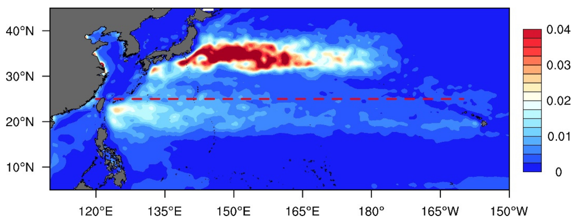
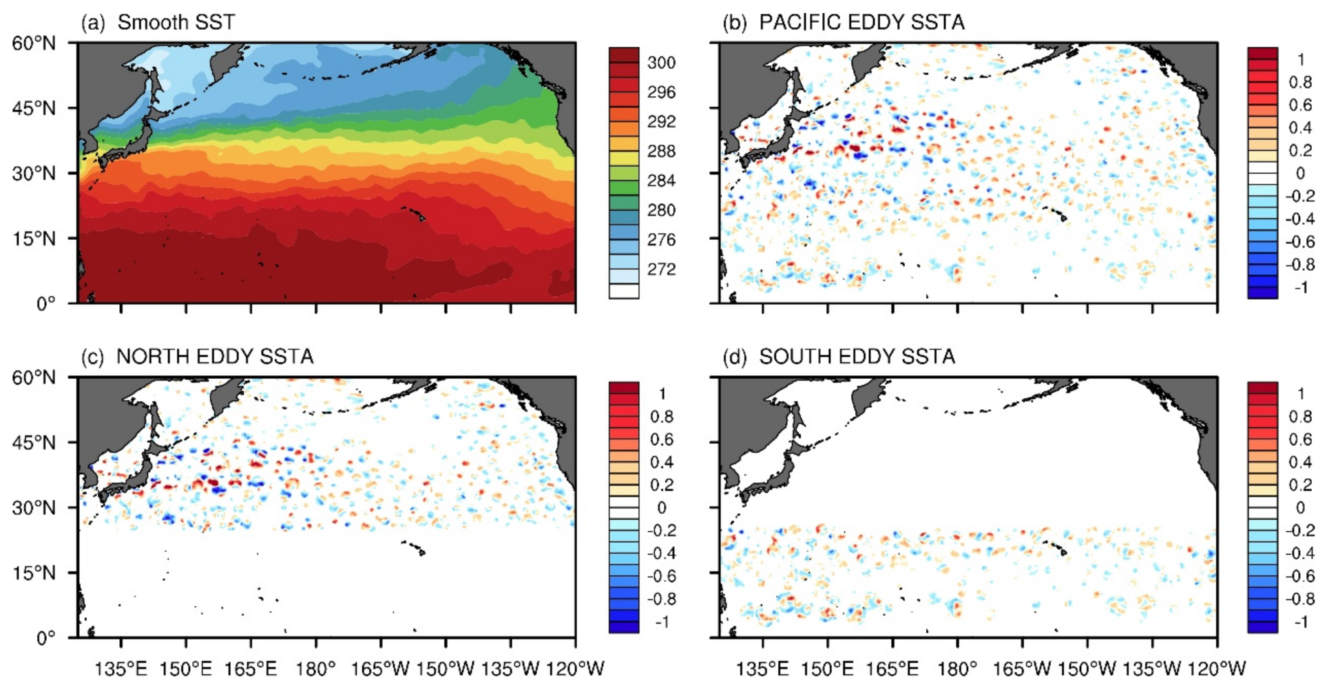
Figure 1. Climatological MAM-mean of high-pass (40–300 day) filtered eddy kinetic energy (EKE) in the ocean (shading; units: m2 s−2) in the North Pacific (NPac) from 2003 to 2008 based on AVISO data. The dashed red line denotes the latitude of 25° N.
Atmosphere 12 00517 g001
Figure 2. Spatial distributions of (a) sea surface temperature (SST) (units: K) in the smoothed-SST (SmthSST) run and (bd) sea surface temperature anomalies (SSTAs) (units: K) associated with the mesoscale oceanic eddies (OEs) in the (b) EddySSTA, (c) EddySSTA+N25N, and (d) EddySSTA+S25N runs at 00 UTC on 1 March 2004.
Atmosphere 12 00517 g002
Figure 3. MAM-mean (a) latent heat flux (LHF) (units: W m−2); (c) sensible heat flux (SHF) (units: W m−2); (e) 300-hPa zonal wind (units: m s−1), and (g) 300-hPa EKE in the atmosphere (units: m2 s−2) in CFSR products during 2003–2008. (b,d,f,h) are the same as (a,c,e,g), respectively, except from the control experiment (CTL).
Atmosphere 12 00517 g003
Figure 4. The 2003 March-mean SSTAs (contours from −1.5 °C to 1.5 °C at an interval of 0.3; solid and dashed contours are for positive and negative anomalies, respectively, and the zero contour is omitted for clarity) and 10-m wind anomalies (shading; units: m s−1) from (a) the OISSTV2 and QuickSCAT datasets and (c) the CTL run. (b) The scatter plot between SSTAs and 10-m wind anomalies in the NPac region (155°–175° E, 35°–45° N; outlined by black dashed lines in the left panels) from (b) the OISSTV2 and QuickSCAT datasets and (d) the CTL run. Each blue dot denotes a model grid box. The red solid line represents the linear regression between the two variables, and its regression coefficient (the slope) is given at the lower-right corner.
Atmosphere 12 00517 g004
Figure 5. MAM-mean differences of (a,b) geopotential heights (GPH) (shading; units: m); (c,d) zonal winds (shading; units: m s−1), and (e,f) storm track at 300 hPa (left) and 850 hPa (right) between EddySSTA and SmthSST runs (EddySSTA minus SmthSST). The contours represent the respective climatological mean from 2003 to 2008 in the CTL run. Hatching denotes that the difference is statistically significant at the 95% confidence level on the basis of the Empirical Monte Carlo (EMC) significance test. Note that the storm tracks at 300 and 850 hPa are defined by the EKE in the atmosphere (units: m2 s−2) and the poleward heat flux v T (units: K m s−1), respectively.
Atmosphere 12 00517 g005
Figure 6. MAM-mean differences of (a) 300-hPa and (c) 850-hPa GPH (shading; units: m) between EddySSTA + N25N and SmthSST runs (EddySSTA + N25N minus SmthSST). The contours represent the corresponding climatological mean from 2003 to 2008 in the CTL run. Hatching denotes that the difference is statistically significant at the 95% confidence level on the basis of the EMC test. (b,d) are the same as (a,c), respectively, except for the differences between EddySSTA + S25N and SmthSST runs (EddySSTA + S25N minus SmthSST).
Atmosphere 12 00517 g006
Figure 7. Same as Figure 6, except for the differences of (a,b) 300-hPa and (c,d) 850-hPa zonal winds.
Atmosphere 12 00517 g007
Figure 8. Vertical cross sections of MAM-mean differences of zonal winds averaged over 135° E–135° W (shading; units: m s−1) between EddySSTA + N25N and SmthSST runs (a) and between EddySSTA + S25N and SmthSST runs (b). The contours represent the climatological mean zonal winds from 2003 to 2008 in the CTL run. Hatching denotes that the difference is statistically significant at the 95% confidence level on the basis of the EMC test.
Atmosphere 12 00517 g008
Figure 9. Differences of mean GPH at 850 hPa (Z850; contour; m; blue solid and red dashed contours are for positive and negative anomalies, respectively, and the zero contour is omitted for clarity) and at 300 hPa (Z300; shading; m) between EddySSTA and SmthSST runs in (a) March; (b) April, and (c) May. Hatching denotes that the difference is statistically significant at the 95% confidence level on the basis of the EMC test.
Atmosphere 12 00517 g009
Figure 10. MAM-mean differences of (a,b) 300-hPa EKE in the atmosphere (shading; units: m2 s−2) and (c,d) 850-hPa transient eddy heat transport ( v T ; shading; units: K m s−1) between EddySSTA + N25N and SmthSST runs (a,c) and between EddySSTA + S25N and SmthSST runs (b,d). The contours represent the corresponding climatological mean from 2003 to 2008 in the CTL run. The hatching denotes that the difference is statistically significant at the 95% confidence level on the basis of the EMC test.
Atmosphere 12 00517 g010
Figure 11. MAM-mean differences of water vapor vertically averaged from 1000 to 850 hPa (shading; units: g kg−1) between EddySSTA + N25N and SmthSST runs (a) and between EddySSTA + S25N and SmthSST runs (b). Hatching denotes that the difference is statistically significant at the 95% confidence level on the basis of the EMC test. The green solid line denotes the lower-level storm track core at 40° N from 150° E to 180° E in the CTL run.
Atmosphere 12 00517 g011
Figure 12. April-mean differences of (a,b) GPH at 850 hPa (Z850; contour; m; blue solid and red dashed contours are for positive and negative anomalies, respectively, and the zero contour is omitted for clarity) and at 300 hPa (Z300; shading; m); (c,d) 300-hPa EKE in the atmosphere (shading; units: m2 s−2), and (e,f) 850-hPa transient eddy heat transport ( v T ; shading; units: K m s−1) between EddySSTA + N25N and SmthSST runs (a,c,e) and between EddySSTA + S25N and SmthSST runs (b,d,f), respectively. The hatching denotes the difference is statistically significant at the 95% confidence level on the basis of the EMC test.
Atmosphere 12 00517 g012
Table 1. Schemes of the numerical experiments.
ExperimentDescription of Experiments
Control experiment (CTL)Observed daily sea surface temperature (SST) is used as the boundary condition of the model
Smoothed-SST experiment (SmthSST)Same as CTL, but with the spatially smoothed SST used as the boundary condition of the model
EddySSTASame as SmthSST, but with sea surface temperature anomalies (SSTAs) associated with the oceanic eddies in the whole north Pacific (NPac) being superimposed on the smoothed SST
EddySSTA + N25NSame as EddySSTA, but with SSTAs associated with the oceanic eddies to the north of 25° N being superimposed on the smoothed SST
EddySSTA + S25NSame as EddySSTA, but with SSTAs associated with the oceanic eddies to the south of 25° N being superimposed on the smoothed SST
Publisher’s Note: MDPI stays neutral with regard to jurisdictional claims in published maps and institutional affiliations.

