Variations in Wave Energy and Amplitudes along the Ray Paths of Barotropic Rossby Waves in Horizontally Non-Uniform Basic Flows

Abstract

A non-divergent barotropic model on a sphere transformed to Mercator coordinates is used to examine the variations in wave energy and amplitude along the energy dispersion paths of barotropic Rossby waves in non-uniform basic flows. Wave energy can be easily solved by specifying the divergence of the group velocity along the corresponding rays. In an analytical non-uniform basic flow that represents the basic features of the observed one at middle latitudes, waves with different periods decay accompanying the decreases in wave energy and amplitude and the increase in the total wavenumber. This implies that the waves are trapped and the energy is eventually absorbed by the basic flow. For the observed non-uniform basic flow that can represent the basic features of the non-divergent wind field at 200 hPa, the situation is more complicated. The significant increase in wave energy can be caused by either the convergence of wave energy or the barotropic energy absorption from the basic flow or both of them. A significant increase in amplitude can also be observed if the total wavenumber varies moderately. This means waves can significantly develop. Waves may decay if both wave energy and amplitude decrease. Waves may propagate without significant developing or decaying to realize a long distance propagation. The propagating waves are mainly caused by oscillating wave energy as well as amplitude.

1. Introduction

Carl Gustaf Rossby’s discovery in the 1930s of a special class of waves that owe their existence to the spherical shape of the Earth, now widely known as Rossby waves, was one of the major breakthroughs in the development of a theoretical understanding of the large scale circulation of the atmosphere and ocean [1]. Rossby waves play an important role in the large scale dynamics of the atmosphere and ocean of the Earth and also different astrophysical objects such as the solar atmosphere and interior, astrophysical discs, rapidly rotating stars and planetary and exoplanetary atmospheres [2].

As for the propagation of Rossby waves, a great deal of research has pointed out that the energy dispersion caused by difference between the group velocity and phase velocity can be applied to interpret many observed atmospheric phenomena (e.g., [3,4]). Hoskins and Karoly [5] firstly applied the wave ray theory to discuss the meridional propagation of stationary Rossby waves and the observed teleconnection patterns in large scale atmospheric circulation. After that, extensive research has focused on the ray paths, wavenumber profiles, wave periods, amplitudes and wave energy of barotropic Rossby waves in horizontally uniform basic flows. For example, Hoskins and Ambrizzi [6] studied stationary Rossby wavenumber profiles and the refraction of ray paths and pointed out the possible existence of a strong waveguide in the Asian jet and a weaker waveguide in the North America and Southern Hemisphere jets. Li and Nathan [7] derived an expression for the disturbance amplitude that depends on the meridional wave scale and northward group velocity, both of which are functions of the slowly varying background flow. Yang and Hoskins [8] further investigated the propagation of Rossby waves of eastward and westward phase speeds. They suggested that westward waves tend to have larger total wavelengths and increased meridional group velocities that benefit a cross-equatorial propagation. Li et al. [9] emphasized the variations in amplitude and wave energy along the ray paths by proposing a new method to calculate the divergence of the group velocity.

Eastward or stationary Rossby waves in a uniform basic flow cannot propagate across the equator regions where observed easterlies prevail. In fact, those Rossby waves only can cross the equator in limited tropical regions where westerly wind (known as the equatorial westerly window) prevails in the winter season. The easterly barrier is inconsistent with the observed interhemispheric teleconnection phenomena (e.g., [10,11,12]). Furthermore, more and more observations suggest that Rossby waves could also propagate across the equator through the strong cross-equatorial flows in the tropical easterly wind regions (e.g., [13,14,15,16]). This involves the propagation of Rossby waves in horizontally non-uniform basic flows.

Karoly [17] extended the horizontally uniform basic state to a horizontally non-uniform one. He focused on the cross-equatorial propagation but neglected amplitude variation due to the complexity of the calculation. Hoskins and Ambrizzi [6] considered the propagation of Rossby waves on a realistic zonally varying flow and they tended to neglect the zonal variation due to the short meridional scale on which the basic flow variation occurs. Li and Nathan [18] examined the extratropical response to low-frequency tropical forcing in a zonally varying basic flow. They found out that it is too complex to derive an explicit expression for amplitude and turned to adopt an alternative local energetics analysis. Li and Li [15] systematically discussed the characteristics of stationary and non-stationary wave propagation in the zonally non-uniform basic flow. They pointed out that stationary waves could propagate through the easterlies with a weak meridional wind to realize the interaction between the Northern and Southern Hemisphere. Li et al. [16] further suggested that the large scale monsoonal background flows play a critical role in the interhemispheric teleconnection. Recently, Li et al. [19] further explored the windows and barriers for cross-equatorial waves by the wave ray ensemble method.

These studies have greatly improved the knowledge of cross-equatorial propagation paths that are concentrated in a few preferred regions with strong cross-equatorial flows. However, the wave ray tracing analysis only provides information on the energy propagation path but leaves wave energy and amplitude of the wave packets undiscussed. It is of importance to identify the variations in wave energy and amplitude [20]. For horizontally uniform basic flows, amplitude can be solved either by deriving the conservation of the wave action [5,21] or by considering the order analysis in a Wentzel-Kramers-Brillouin (WKB) solution [7]. For horizontally non-uniform basic flows, however, there is not a simple mathematical expression describing the relationship between amplitude, wave scale and wave frequency yet due to the complexity of the zonally asymmetric basic flow [18]. As a result, there is no relevant research on wave energy and amplitude variations along the wave rays. Recently, Li et al. [9] calculated wave energy and amplitude along the wave rays under horizontally uniform basic flows to discuss developing Rossby waves by applying the criterion of Lu and Zeng [20], which states that developing waves should accompany the growth of both wave energy and amplitude. Inspired by their work, this paper tries to discuss the variations in wave energy and amplitude along the wave rays by deriving the wave energy equation in the horizontally non-uniform basic flow.

2. Wave Energy Equation in the Non-Uniform Basic Flow

Following Karoly [17], the non-divergent barotropic vorticity equation in the Mercator projection of the sphere is linearized for a time-mean basic state with a stream function $\overline{\psi }\left(x,y\right)$, which is a function of both longitude and latitude. The perturbation stream function $\psi$ could be written as:

$$\left(\frac{\partial }{\partial t}+{\overline{u}}_M\frac{\partial }{\partial x}+{\overline{v}}_M\frac{\partial }{\partial y}\right){\nabla }^2\psi +{\overline{q}}_y\frac{\partial \psi }{\partial x}-{\overline{q}}_x\frac{\partial \psi }{\partial y}=0$$

(1)

where ${\overrightarrow{v}}_M=\left({\overline{u}}_M,{\overline{v}}_M\right)$ and ${\nabla }^2$ are the velocity and Laplacian operator in the Mercator projection, respectively; $\overline{q}={\nabla }^2\overline{\psi }/{\cos }^2\theta +2\overline{\mathsf{\Omega }}\sin \theta$ is the absolute vorticity on the sphere; ${\overline{q}}_x$ and ${\overline{q}}_y$ are the derivatives with respect to $x$ and $y$, respectively; $\overline{\mathsf{\Omega }}$ is the Earth’s rotation rate.

Assuming that amplitude of the wave packet is a slowly varying function of time and space, the single wave solution of Equation (1) is:

$$\psi =A(T,X,Y)e^{i\left(kx+ly-\omega t\right)}$$

(2)

where $A$ is amplitude of the wave packet; $(T,X,Y)=\epsilon \left(t,x,y\right)$ and $\epsilon$ are the ratio between the length scale of the wave packet and the length scale of the mean flow and satisfies $\epsilon \ll 1$. It denotes that, compared with the perturbation itself, the time and spatial scales of amplitude vary slowly. Applying the WKB method, we expand $A$ into a series of $\epsilon$, namely $A=A_0+\epsilon A_1+{\epsilon }^2{A}_2+\dots$ where $A_i$ and $i=0,1,2,\cdots$ are the coefficients. Substituting Equation (2) into Equation (1) and retaining the terms containing $A_0$ (zeroth-order approximation), we derive the dispersion relation (see Appendix A):

$$\omega ={\overline{u}}_{M}k+{\overline{v}}_{M}l+\frac{{\overline{q}}_{x}l-{\overline{q}}_{y}k}{k^2+l^2}\equiv \mathsf{\Omega }\left(k,l,X,Y\right)$$

(3)

where $\left(k,l\right)$ are the zonal and meridional wavenumbers, respectively, and $\omega$ is the circular frequency. The zonal and meridional components of the group velocity take the form:

$$c_{gx}=\frac{\partial \omega }{\partial k}={\overline{u}}_M+\frac{\left(k^2-l^2\right){\overline{q}}_y-2kl{\overline{q}}_x}{K^4}$$

(4)

$$c_{gy}=\frac{\partial \omega }{\partial l}={\overline{v}}_M+\frac{2kl{\overline{q}}_y+\left(k^2-l^2\right){\overline{q}}_x}{K^4}$$

(5)

where $K=\sqrt{k^2+l^2}$ is the total wavenumber. According to Whitham [22], the evolution of $k$ and $l$ satisfy:

$$\frac{D_{g}k}{Dt}=-\frac{\partial \mathsf{\Omega }}{\partial x}=-k\frac{\partial {\overline{u}}_M}{\partial x}-l\frac{\partial {\overline{v}}_M}{\partial x}-\frac{{\overline{q}}_{xx}l-{\overline{q}}_{yx}k}{K^2}$$

(6)

$$\frac{D_{g}l}{Dt}=-\frac{\partial \mathsf{\Omega }}{\partial y}=-k\frac{\partial {\overline{u}}_M}{\partial y}-l\frac{\partial {\overline{v}}_M}{\partial y}-\frac{{\overline{q}}_{xy}l-{\overline{q}}_{yy}k}{K^2}$$

(7)

where $D_g/Dt=\partial /\partial t+c_{gx}\partial /\partial x+c_{gy}\partial /\partial y$ is the material derivative along the group velocity. The above four equations determine a spatial curve known as a ray. As the basic flow is $x$-dependent, the zonal wavenumber $k$ is not conserved along the wave ray. Karoly [17] first derived these equations and solved the ray trajectories on the sphere. Li and Nathan [18] further analyzed the limitations of the ray tracing method. Li and Li [15] and Li et al. [16] systematically discussed the spatial and periodic characteristics of wave energy propagation.

The wave energy equation could be finally derived by taking the first-order approximation (see Appendix A):

$$\frac{\partial E}{\partial T}+\nabla \cdot \left(E{\overrightarrow{c}}_g\right)=\frac{1}{2}{A}_0^2\left(k^2\frac{\partial {\overline{u}}_M}{\partial X}+l^2\frac{\partial {\overline{v}}_M}{\partial Y}+kl\frac{\partial {\overline{v}}_M}{\partial X}+kl\frac{\partial {\overline{u}}_M}{\partial Y}\right)$$

(8)

where $E=\frac{1}{4}{K}^2{A}_0^2$ is the wave energy density of the barotropic Rossby wave, an average of wave energy in a period. If ${\overline{u}}_M={\overline{u}}_M\left(Y\right)$ and ${\overline{v}}_M\equiv 0$, then Equation (8) reduces to:

$$\frac{\partial E}{\partial T}+\nabla \cdot \left(E{\overrightarrow{c}}_g\right)=\frac{1}{2}{A}_0^2\left(kl\frac{\partial {\overline{u}}_M}{\partial Y}\right).$$

(9)

Equation (9) is the wave energy equation for a horizontally uniform basic flow and could be applied to analyze the development of Rossby waves (e.g., see [20,23]). Define $F=\frac{E}{{\omega }^{\prime }}$ as the wave action density and then the wave energy equation could be transformed to the wave action equation:

$$\frac{\partial F}{\partial T}+\nabla \left(F{\overrightarrow{c}}_g\right)+G=0$$

(10)

where:

$$\begin{array}{c}G=\frac{1}{4}\frac{1}{{{\omega }^{\prime }}^2}{A}_0^2\left[{\overline{q}}_y\left(k\frac{\partial {\overline{u}}_M}{\partial X}+l\frac{\partial {\overline{v}}_M}{\partial X}\right)-{\overline{q}}_x\left(k\frac{\partial {\overline{u}}_M}{\partial Y}+l\frac{\partial {\overline{v}}_M}{\partial Y}\right)\right]\\ +\frac{1}{4}\frac{1}{{{\omega }^{\prime }}^2}{A}_0^2\left[{\overline{u}}_M\left(l\frac{\partial {\overline{q}}_x}{\partial X}-k\frac{\partial {\overline{q}}_y}{\partial X}\right)+{\overline{v}}_M\left(l\frac{\partial {\overline{q}}_x}{\partial Y}-k\frac{\partial {\overline{q}}_y}{\partial Y}\right)\right]\end{array}$$

(11)

where ${\omega }^{\prime }\equiv \omega -{\overline{u}}_{M}k-{\overline{v}}_{M}l=\frac{{\overline{q}}_{x}l-{\overline{q}}_{y}k}{k^2+l^2}$ is the intrinsic frequency.

Young and Rhines [24] derived similar wave energy and action equations for Rossby wave trains in an ocean of varying depth on a $\beta$-plane. They further pointed out that wave action is not conserved in the most general case. Plumb [25] also noted that no conservation law exists if the basic state is not uniform in any one direction. According to Equation (10), we could obtain the similar conclusion that the wave action is no longer conserved for a horizontally non-uniform basic flow only if it satisfies $G=0$. This is a major difference compared with the horizontally uniform basic flow.

Karoly [17] noticed that the complex expressions for wave action and energy prohibited a simple expression of amplitude as in the horizontally uniform basic flow. Therefore, he mainly analyzed the ray paths but left wave energy and amplitude undiscussed. Li and Nathan [18] realized the importance of the variations of wave energy and amplitude along the wave rays. However, they did not derive corresponding expressions but instead applied an alternative local energetics analysis to feature the wave amplitude.

We can rewrite Equation (8) as:

$$\frac{1}{E}\frac{D_{g}E}{D_{g}T}=-\nabla \cdot {\overrightarrow{c}}_g+\frac{2}{K^2}\left(k^2\frac{\partial {\overline{u}}_M}{\partial X}+kl\frac{\partial {\overline{u}}_M}{\partial Y}+l^2\frac{\partial {\overline{v}}_M}{\partial Y}+kl\frac{\partial {\overline{v}}_M}{\partial X}\right).$$

(12)

Equation (12) demonstrates that the variation of wave energy along the ray is determined by the sum of the divergence of the group velocity (the first term at the right hand) and the products of the horizontal scales and the gradients of the non-uniform basic flow (the second term). As the group velocity is the velocity of the energy dispersion, its divergence or convergence denotes wave energy divergence or convergence. Therefore, wave energy increases (decreases) if the energy is concentrated (dispersed) along a marching ray. The second term represents the effects of the wave basic flow interaction [25]. The wave gains (loses) barotropic energy from (to) the basic flow when the term is larger (smaller) than zero.

Equation (12) provides a possible way to calculate wave energy and hence amplitude along a ray. However, we cannot directly differentiate Equations (4) and (5) to calculate the divergence of the group velocity because the group velocity values neighboring a ray are unknown [26]. Inspired by Lighthill [26] and Karoly and Hoskins [27] who dealt with the situation that satisfies $\nabla \cdot \overrightarrow{c_g}=0$, we propose an available method [9] to calculate the divergence of the group velocity:

$$\nabla \cdot \overrightarrow{c_g}=\underset{\delta t\to 0}{\lim }\frac{{\left(\overrightarrow{c_g}\cdot \overrightarrow{\delta S}\right)}_{t+\delta t}-{\left(\overrightarrow{c_g}\cdot \overrightarrow{\delta S}\right)}_t}{{\left(\left|\overrightarrow{c_g}\right|\cdot \left|\overrightarrow{\delta S}\right|\right)}_t\cdot \delta t}$$

(13)

where subscript $t$ denotes time and $\delta t$ represents a short time interval; $\overrightarrow{\delta S}$ denotes the unit area that is perpendicular to the group velocity. Equation (13) reduces to the method adopted by Lighthill [26] and Karoly and Hoskins [27] if the divergence of the group velocity equals zero. As the group velocity along a ray is known, we could easily solve the divergence of the group velocity and hence wave energy and amplitude.

3. Results

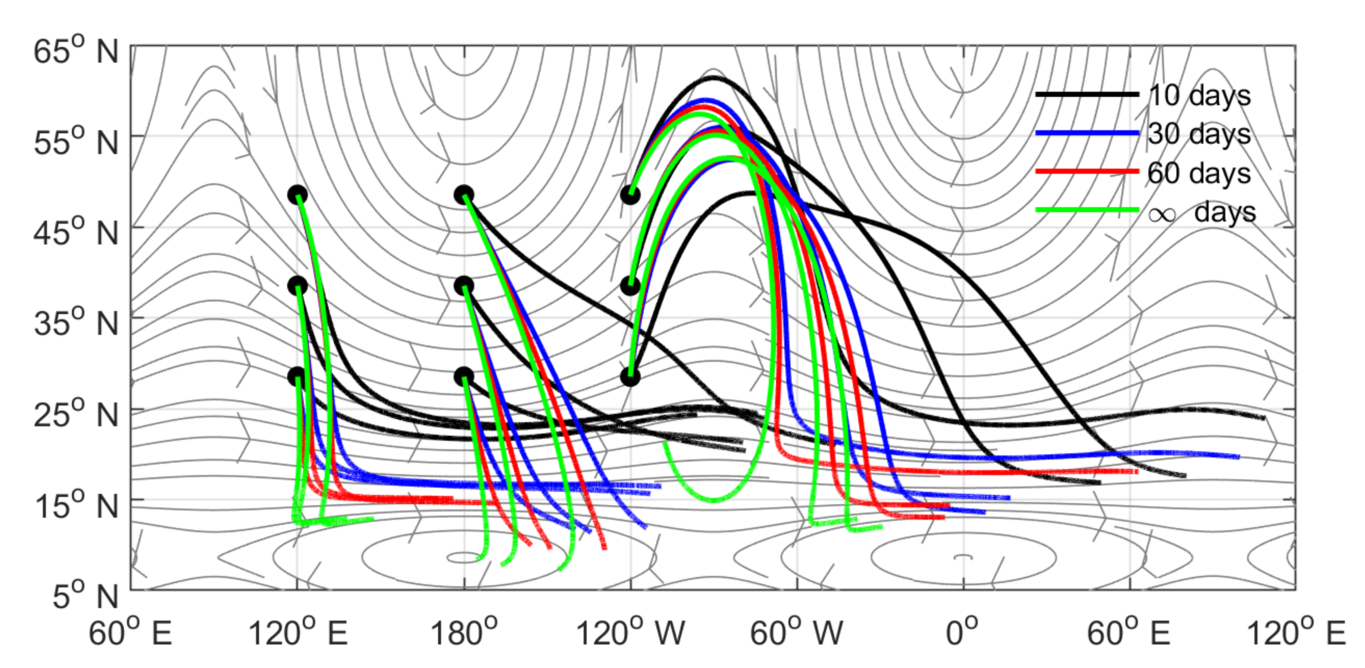
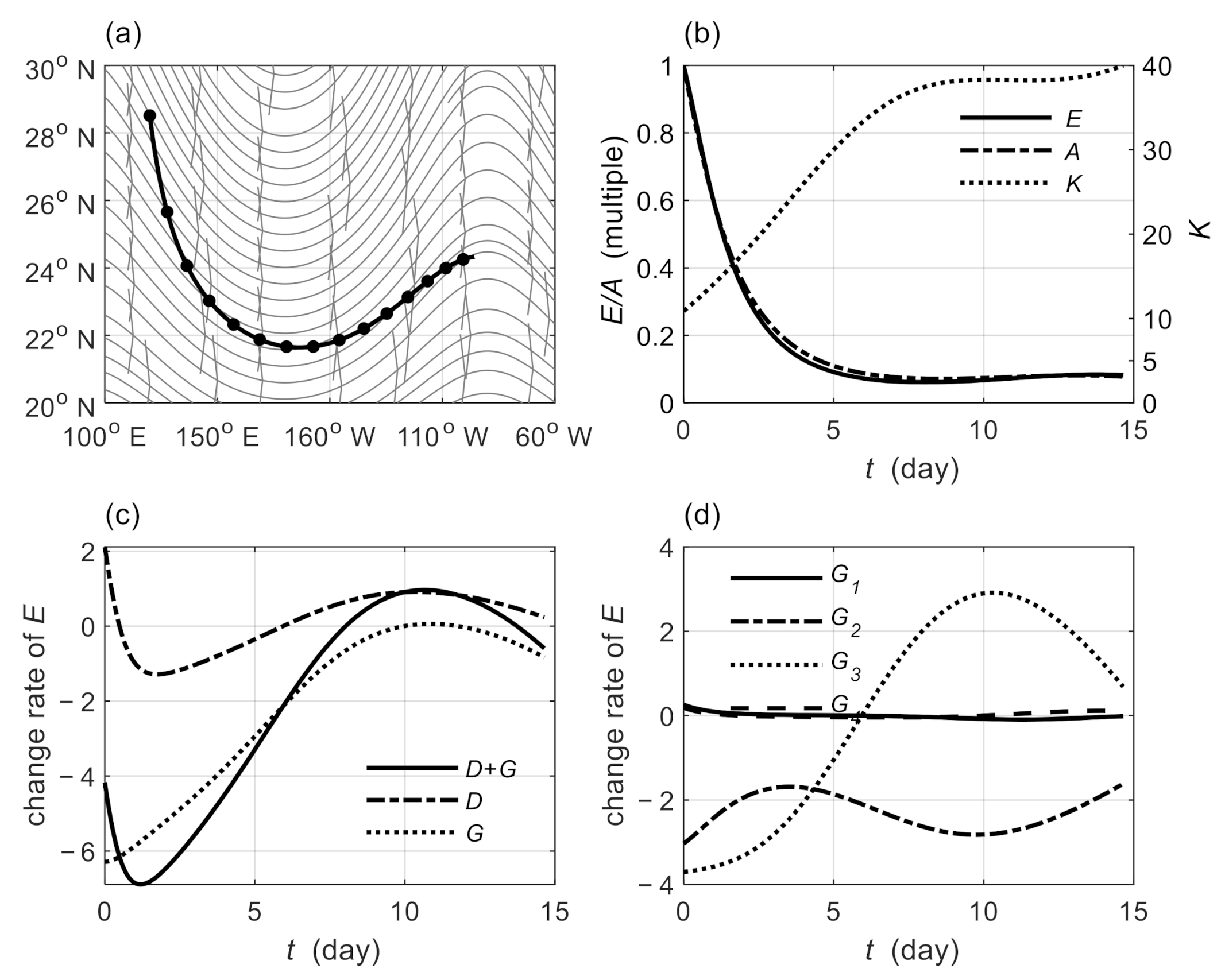
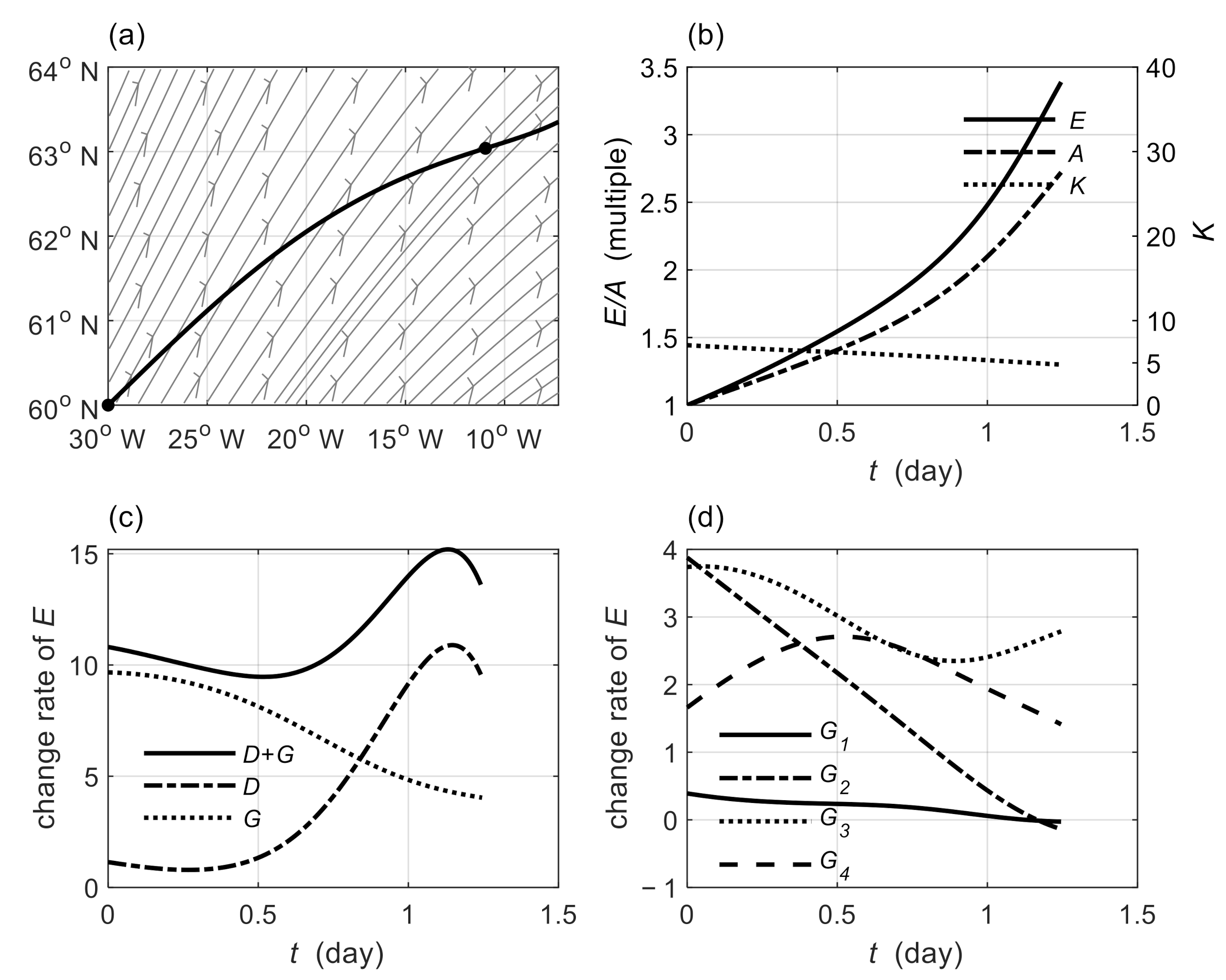
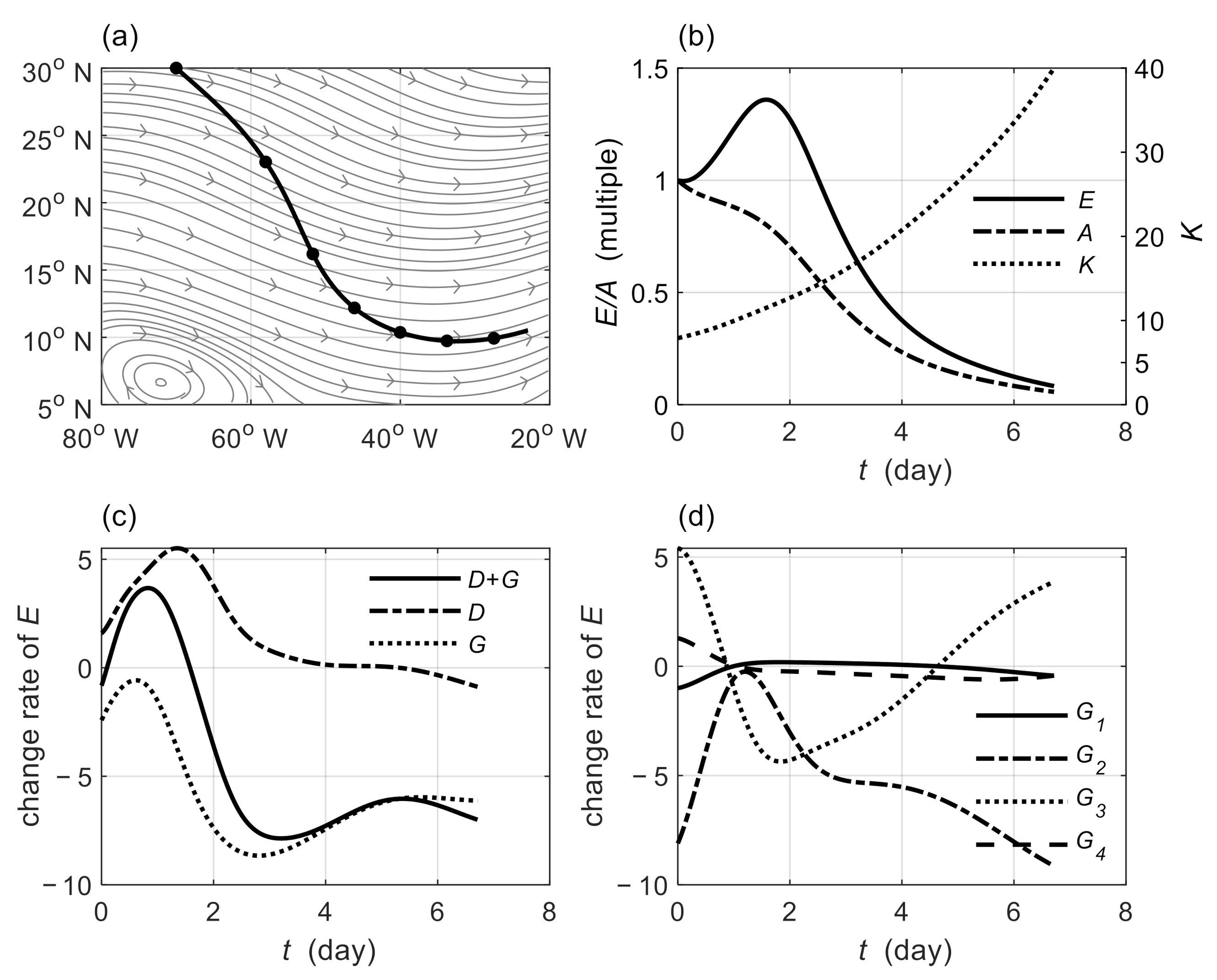
3.1. Analytical Horizontally Non-Uniform Basic Flow

Climatological westerly jet prevails at the middle latitudes with two centers located at the eastern and western northern hemisphere, respectively. An analytical zonal u-wind is specified to feature the distribution. It is written as:

$$\overline{u}=Y\left(y\right)X\left(\lambda \right)$$

(14)

where:

$$Y\left(y\right)=18\sin \left[\frac{3}{2}\pi \left(1+y\right)\right]+14\left(1-y^2\right)$$

(15)

$$X\left(\lambda \right)=\frac{1}{4}\cos 2\lambda +\frac{3}{4}$$

(16)

are meridional and zonal distributions, respectively. The profile $Y\left(y\right)$ where $y=\sin \phi$ is taken from Schneider and Watterson [28] with a maximum westerly speed of about 26.1 m/s at 38.5° N and a maximum easterly speed of 4 m/s at the equator. After multiplying by $X\left(\lambda \right)$ where $\lambda$ is the longitude, the u-wind speed varies with the longitude to form two jet stream centers located at 0°, 38.5° N and 180°, 38.5° N with a maximum speed of about 26.1 m/s (Figure S1a online). The v-wind could be solved by applying the incompressible continuity equation:

$$\overline{v}=-\frac{1}{\cos \phi }{X}^{\prime }\left(\lambda \right){\displaystyle \int Y\left(y\right)}d\phi$$

(17)

where $X^{\prime }$ means the derivative of $X$ with respect to $\lambda$. Equation (17) cannot be analytically expressed due to the complex form of $Y$. It is obvious that the zonal distribution of the v-wind obeys a sinusoidal type with alternative northerlies and southerlies. The meridional distribution indicates that the v-wind speed is reasonably about 4 m/s near the jet axis (Figure S1b online). However, the v-wind speed approaches to an unrealistic maximum value near the North Pole. Therefore, it is more suitable to analyze regions nearby the jet stream, which is deemed as a most important waveguide for Rossby waves.

Here, the specified analytical basic flow is applied based on two reasons. The first one is that it is simple (although simple, it can represent the main features of the basic flow). We can analyze the ray paths, amplitude and wave energy to summarize a few general and fundamental propagating characteristics. The second one is that it can provide a reference to the results for the observed basic flow. Hoskins and Karoly [9] pointed out that analytical results are necessary because many of the results obtained from the observed basic flow are of little difference from those obtained from an analytical one. For a zonally non-uniform basic flow, there is yet no relevant research on varying wave energy and amplitude. Therefore, it is necessary to summarize a few basic conclusions for these variations along the rays before analyzing the observed ones.

We calculate rays with different periods that are generated from an array of points located near the jet stream (Figure 1). Both wave energy and amplitude eventually decrease along all of the marching rays, suggesting waves are decaying. The waves are eventually trapped and their energy is absorbed by the basic flow. As the situation is quite similar for waves that generate from the array, we can only analyze a wave sourced from 120° E, 28.5° N and with a period T = 10 days as an example (Figure 2). The ray moves southward toward a turning point and then turns toward the northeast within around 15 days, basically following the streamlines of the basic wind (Figure 2a). Both wave energy and amplitude continuously decrease to about a tenth of the initial values (Figure 2b), suggesting a decaying wave. As we only discuss large scale Rossby waves, we terminate the calculation when the total wavenumber is larger than 40, which means the corresponding horizontal scale is less than around 1000 km. The decreasing wave energy as well as the increasing total wavenumber contributes to the decreasing amplitude. The decrease in wave energy is jointly determined by the divergence of the group velocity (D) and the energy budget from the basic flow (G) (Figure 2c). D continuously declines to the minimum negative value and rebounds to the maximum positive value and then declines again. It denotes that wave energy alternately concentrates and disperses along the marching ray. G, however, continuously increases to the maximum positive value that is very close to zero and then decreases. This behavior indicates that the wave generally loses its energy to the basic flow. The sum of the two varies as D.

The form of the energy budget is complex in the non-uniform basic flow. It is composed of four items (labelled as G₁, G₂, G₃ and G₄, respectively), which associate with $\overline{v^{\prime }{v}^{\prime }}\frac{\partial {\overline{u}}_M}{\partial X}$, $\overline{u^{\prime }{v}^{\prime }}\frac{\partial {\overline{u}}_M}{\partial Y}$, $\overline{u^{\prime }{u}^{\prime }}\frac{\partial {\overline{v}}_M}{\partial Y}$ and $\overline{u^{\prime }{v}^{\prime }}\frac{\partial {\overline{v}}_M}{\partial X}$, respectively (see Appendix B). G₁ and G₄ are relatively small due to the small derivative of the basic flow in longitude (Figure 2d) and can be neglected compared with G₂ and G₃. This implies that although there exists a zonal variation in the basic flow, its effect on wave energy is still limited and can be neglected. During the propagating period, the wave is located at the south of the jet axis ($\frac{\partial {\overline{u}}_M}{\partial Y}>0$) and keeps a trailing structure (defined by kl < 0). Therefore, G₂ is smaller than zero. Meanwhile, the derivative of the meridional wind in latitude becomes larger than zero at around the sixth day, which leads to the same variation in G₃. Both G₂ and G₃ jointly determine the variation of G. Now it is clear that the structure of the basic flow (especially the derivatives in latitude) and the structure of the wave contribute to the energy budget from the basic flow. The waves originating from the same point but with different periods (T = 30, 60 and infinity days; see Figures S2–S4 online) show very similar features.

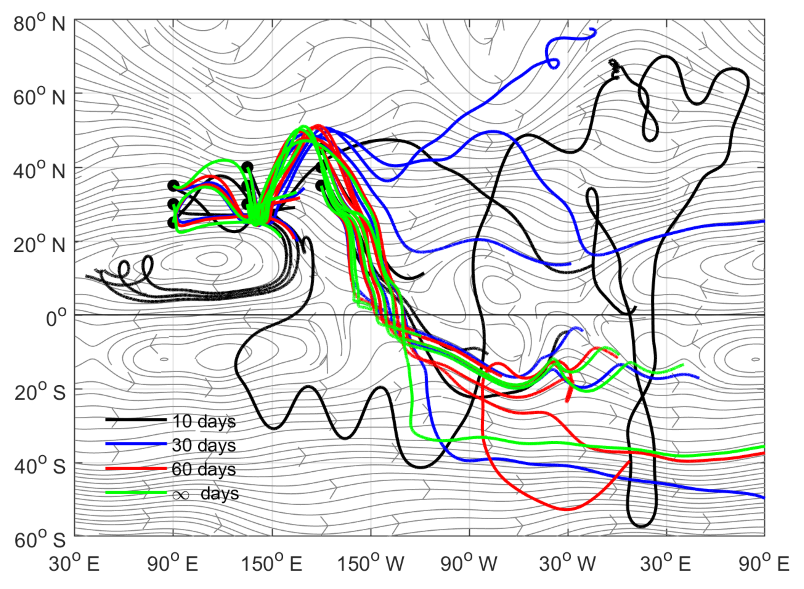
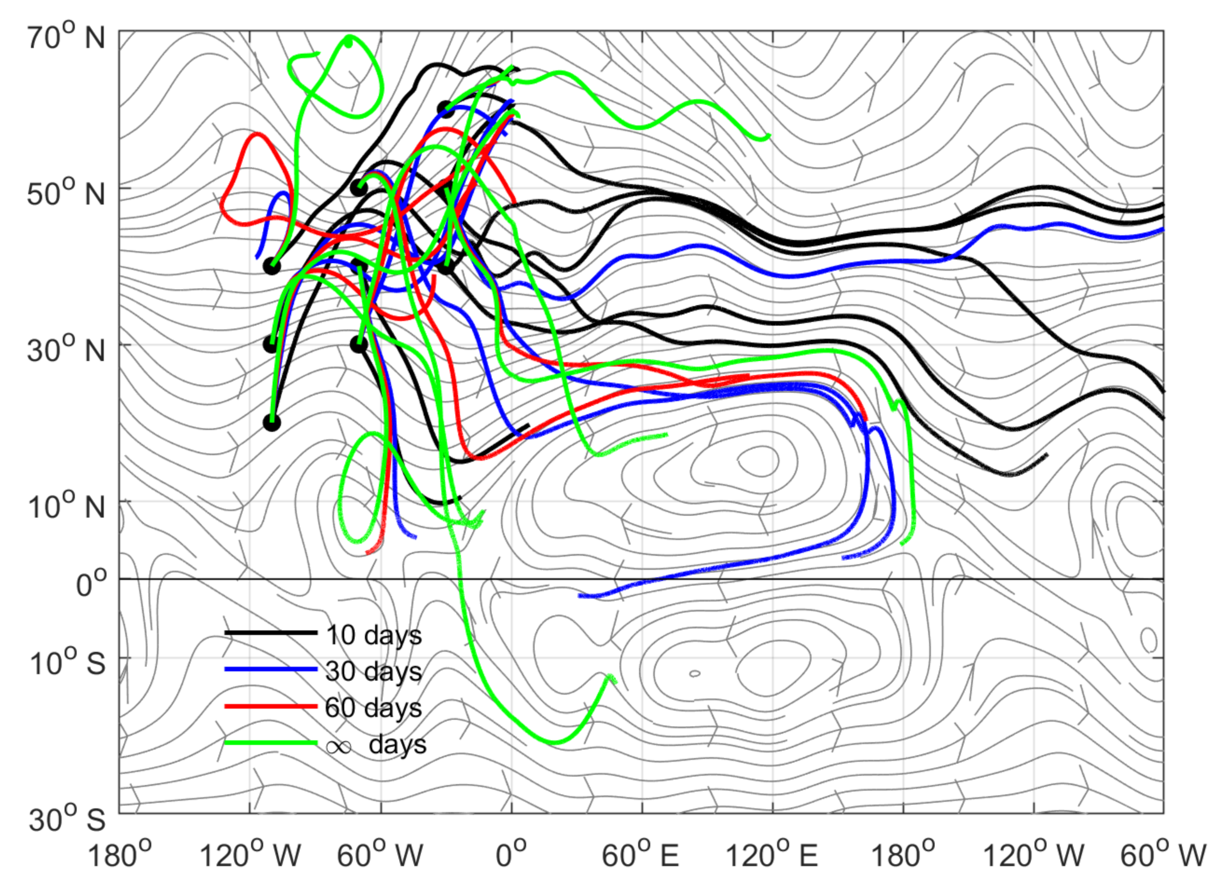
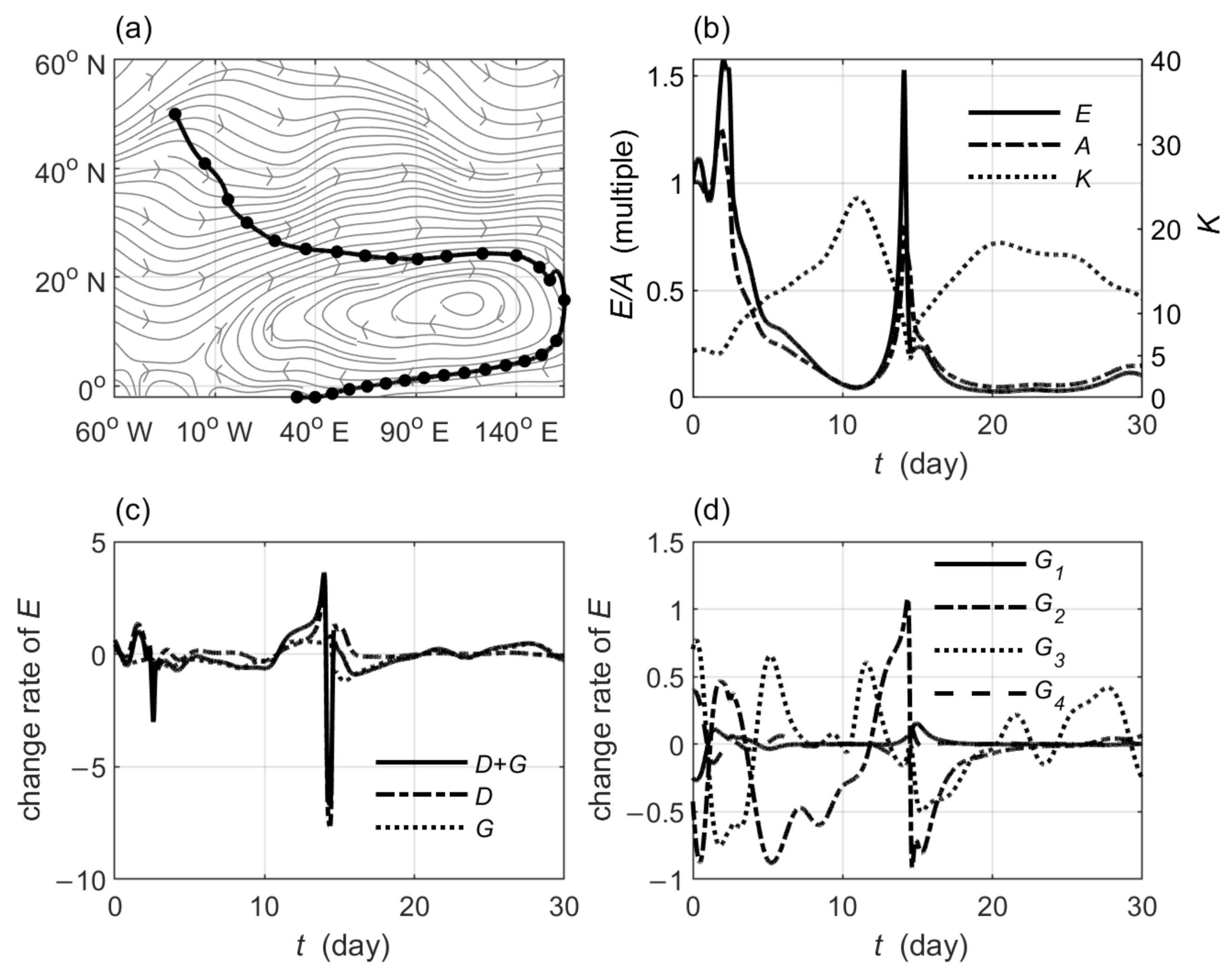
3.2. Observed Horizontally Non-Uniform Basic Flow

We further calculate variations in wave energy and amplitude by placing two arrays of wave sources located along the westerly jet stream in the eastern and western hemispheres, respectively. The horizontally non-uniform basic flow (Figure S5) is taken from NCEP Reanalysis data [29] provided by the NOAA/OAR/ESRL PSD, Boulder, Colorado, USA, from their website at https://www.esrl.noaa.gov/psd/ (accessed on 3 April 2021). Compared with the analytical results, rays generating from different locations with different periods behave quite differently (Figure 3 and Figure 4). Along the marching rays, both wave energy and amplitude show complex variations that can be classified into three types. In the first type, both wave energy and amplitude simultaneously increase to exceed a critical value. The critical value is set to the natural constant (e) times the initial value. It is clear that a wave can develop significantly if both its wave energy and amplitude dramatically increase. In the second type, both wave energy and amplitude eventually simultaneously decrease accompanied by an increasing total wavenumber. The wave decays and is absorbed by the basic flow as the analytical basic flow does. In the third type, both wave energy and amplitude oscillate. The rays generally follow the basic flow to propagate a long distance. The basic flow works as a waveguide.

Figure 5 shows an example of a significantly developing wave. The source is set to 30° W, 60° N with a period of T = 30 days. The ray (Figure 5a) moves northeast until both wave energy and amplitude (Figure 5b) exceed the critical value to terminate the calculation within around 1.3 days. Both D and G are positive and play matched roles in determining the significantly increasing wave energy (Figure 5c). Furthermore, the four components of the energy budget are all positive and are equally important although G₄ seems a little weaker (Figure 5d). Therefore, wave energy dramatically increases along the marching ray due to continuously convergent energy and absorbing barotropic energy from the basic flow by the action of eddies. The increase in amplitude is caused by the increase in wave energy and the decrease in the total wavenumber or increase in the wave scale. Another example of a significantly developing wave (Figure S6 online) shows quite similar features. It seems that a wave that can significantly develop is in a very favorable environment in which not only its own energy is concentrated but also it can efficiently absorb the barotropic energy from the basic flow.Figure 6 shows an example of a decaying wave. The wave source is set to 70° W, 30° N with a period of T = 10 days. The ray (Figure 6a) propagates southeast to around 20° W, 20° N within around seven days. Along the marching ray, wave energy increases to the maximum value of 1.3 times the initial value and then decreases until the total wavenumber exceeds 40 to terminate the ray (Figure 6b). The increase in wave energy is caused by the convergent wave energy while the decrease is mainly caused by the energy absorption by the basic flow (Figure 6c). Furthermore, the loss of wave energy is mainly determined by G₂ and G₃ (Figure 6d), corresponding with the energy budget that associates with the derivatives of the basic flow with respect to latitude. The role of the momentum transports that associate with the derivatives with respect to longitude (G₁ and G₄) is very weak and can be neglected. Amplitude, however, decreases at the beginning time due to a more dramatic increase in the total wavenumber than in wave energy. Amplitude continuously decreases when wave energy decreases and the total wavenumber continuously increases. Another example of a decaying wave (Figure S7 online) also presents quite similar features. The energy of a decaying wave is gradually absorbed by the basic flow, accompanied by a gradually increasing total wavenumber or a shrinking wave scale. The eventual result is that the wave is trapped by the basic flow.

Figure 7 shows an example of a propagating wave. Here, the propagating wave means that it neither significantly develops nor decays in the 30 day integration period. The wave source is set to 30° W, 50° N with a period of T = 30 days. The ray (Figure 7a) moves southeast to the north margin of the anticyclone circulation centered around 120° E, 15° N within around 10 days. It then basically follows the airstreams of the anticyclone to the tropical easterlies and propagates westward to cross the equator eventually. Wave energy (Figure 7b) oscillates up and down along the marching ray (Figure 7c). The sharp increase or decrease in wave energy is mainly determined by the energy convergence or divergence due to the variations in the group velocity while the gradual increase or decrease is mainly the result of the energy budget from the basic flow. Similar to the previous decaying wave case, the eddy momentum transports that associate with the meridional gradients of the basic flow (G₂ and G₃) play a more dominant role in determining the energy budget from the basic flow (Figure 7d). Different from the previous decaying case, the energy budget oscillates about zero, which determines the oscillation in wave energy. Amplitude (Figure 7b) varies in a similar way to wave energy. Although the total wavenumber also oscillates, it plays a minor role in determining amplitude. We also present another example of a propagating wave (Figure S8 online). The result is similar.

4. Conclusions

This paper investigated the variations in wave energy and amplitude along rays that were generated at different locations in both the analytical and observed horizontally non-uniform jet streams. The wave energy equation in the horizontally non-uniform basic flow was first derived. This equation suggested that the variability of wave energy along a ray was jointly determined by the divergence of the group velocity and the product of the wave scale and the gradients of the basic flow, manifesting the energy divergence or convergence and the eddy momentum transport, respectively. Following our previous study [9], the divergence of the group velocity was expressed as a ratio between the difference in the group velocity flux and the volume it passed through during a short time interval. This method made it easy to solve wave energy and hence amplitude.

The variations of wave energy and amplitude along rays in an analytical non-uniform basic flow were analyzed first. The results suggested that waves decayed, accompanied by shrinking horizontal scale. They were trapped and their wave energy was absorbed by the basic flow. A further analysis suggested that the decrease in wave energy was mainly caused by the energy lost to the basic flow through the activity of eddies that associated with the meridional gradients of the basic flow.

The results for the observed westerly jet stream suggested that waves could either significantly develop or decay or propagate a long distance. For developing waves, the significant increase in wave energy was jointly determined by the energy convergence and the positive eddy momentum transport although any one of the two factors could play a certain negative role in a certain period. Wave energy could significantly increase within a short time period due to a beneficial wave structure and a basic flow distribution. The increase in amplitude was mainly determined by the increase in wave energy because the increase in the total wavenumber was moderate. For decaying waves, both wave energy and amplitude eventually decreased, accompanied by an increasing total wavenumber that exceeded 40 to terminate the ray. The waves generally lost their energy to the basic flow through the negative eddy momentum transport and were trapped by the basic flow. For propagating waves, both wave energy and amplitude oscillated as well as the total wavenumber. The waves could propagate a long distance and even cross the equator to cause an interaction between hemispheres. The oscillating wave energy was the result of the oscillating energy divergence and the eddy momentum transport.

5. Discussion

The above results show that waves can either develop or decay or propagate. However, they are still insufficient to make a specific conclusion as to whether a wave with a specific period and a specific starting point develops or decays or propagates. Considering we can calculate both wave energy and amplitude along a specific ray, we may not need to summarize more specific conclusions. A developing wave is defined as the simultaneous increase in wave energy and amplitude to exceed a critical value. However, the criterion seems more suitable in a global analysis of the perturbation development. According to Lu and Zeng [17], the concentration of perturbation energy in local areas can also bring transient severe weather phenomena. Therefore, it needs more specific analyses and discussions on the definition of the developing wave. Only waves located along the jet stream axis were considered. Waves from the tropics and subtropics have a significant impact on the extratropical regions (e.g., see [15]). Finally, according to Besedina and Popel [30], the velocity of cyclonic vortices has a non-zero component in the motion direction from the equator to the Earth’s pole due to an abrupt decreasing tropopause in the subtropical region. They proposed a mechanism by applying the soliton solutions to the Charney–Obukhov equations (Rossby vortices) and highlighted the effect of the Ekman pumping by friction in the boundary layer. Due to the limitation of the barotropic atmosphere, this study does not investigate the vertical propagation of Rossby waves and the corresponding variations in wave energy and amplitude. Solutions in the three-dimensional quasi-geostrophic potential vorticity equation would benefit this. All of them deserve further study.

On the other hand, all rotating celestial fluid bodies should contain Rossby waves because they are inherent to rotating stratified spheres of fluid or plasma [31,32]. For example, solar Rossby waves propagate and are strongly influenced by the magnetic fields that are almost ubiquitous in the Sun’s atmosphere [33]. The resulting magneto-hydrodynamic (MHD) Rossby waves can interact with differential rotation and toroidal fields to sustain quasi-periodic tachocline non-linear oscillations (TNOs) that occur due to back-and-forth energy exchanges among potential, kinetic and magnetic energies [34,35]. There is a strong connection between longitudinally propagating MHD Rossby waves in the tachocline and surface manifestations in the form of similarly propagating coronal holes and patterns of bright points [36]. These active regions of the sun appear at certain latitude-longitude locations and should accompany the intensified wave energy and amplitude of MHD Rossby waves that propagate there.

According to this study, Rossby waves may also develop significantly at certain latitude-longitude locations. There are a few similarities and differences between this study and TNOs. For the differences, TNOs have been modelled by applying a fully non-linear MHD shallow water system in which variables needed to be expanded in terms of vector and scalar spherical harmonics in order to solve the equations [24,37]. They were similar to the non-linear Orr mechanism that states that even though a modal instability mechanism does not exist, it is possible to obtain an initial value problem leading to an arbitrarily large disturbance growth [38]. Differently, this study used a modal (single wave) solution to derive the dispersion relation and wave energy equation for a Rossby wave with a specified wavenumber and period. TNOs deal with a non-linear system while the modal solution is based on the linearized system. For the similarities, as TNOs are solved by expanding the system in a series, they can link the modal solution by discussing any term (e.g., wavenumber equals 2) in the series. Certain terms may be dominant in the series (e.g., stationary Rossby waves in the Earth’s atmosphere generally have small wavenumbers). This meant that we could simplify the system by analyzing corresponding terms in the series. Actually, we know that MHD Rossby waves also have small wavenumbers, representing a large scale motion [37]. Finally, the total energy (potential plus kinetic plus magnetic) is conserved for MHD Rossby waves although potential vorticity is not conserved [33]. This implies that we also can build conserved variables as we do for Rossby waves in the Earth’s atmosphere. By doing this, it will provide a broader application beyond the atmospheric community.

References

1. Chelton, D.B.; Schlax, M.G. Global observations of oceanic rossby waves. Science 1996, 272, 234–238. [Google Scholar] [CrossRef]
2. Zaqarashvili, T.V.; Albekioni, M.; Ballester, J.L.; Bekki, Y.; Biancofiore, L.; Birch, A.C.; Dikpati, M.; Gizon, L.; Gurgenashvili, E.; Heifetz, E.; et al. Rossby waves in astrophysics. Space Sci. Rev. 2021, 217, 1–93. [Google Scholar] [CrossRef]
3. Yeh, T. On energy dispersion in the amtosphere. J. Meteorol. 1949, 6, 1–16. [Google Scholar] [CrossRef] [Green Version]
4. Longuet-Higgins, M.S. Planetary waves on a rotating sphere. R. Soc. Lond. Ser. A Math. Phys. Sci. 1964, 279, 446–473. [Google Scholar]
5. Hoskins, B.J.; Karoly, D.J. The steady linear response of a spherical atmosphere to thermal and orographic forcing. J. Atmos. Sci. 1981, 38, 1179. [Google Scholar] [CrossRef] [Green Version]
6. Hoskins, B.J.; Ambrizzi, T. Rossby wave propagation on a realistic longitudinally varying flow. J. Atmos. Sci. 1993, 50, 1661–1671. [Google Scholar] [CrossRef] [Green Version]
7. Li, L.; Nathan, T.R. The global atmospheric response to low-frequency tropical forcing: Zonally averaged basic states. J. Atmos. Sci. 1994, 51, 3412–3426. [Google Scholar] [CrossRef] [Green Version]
8. Yang, G.; Hoskins, B.J. Propagation of rossby waves of nonzero frequency. J. Atmos. Sci. 1996, 53, 2365–2378. [Google Scholar] [CrossRef] [Green Version]
9. Li, Y.; Chao, J.; Kang, Y. Variations in wave energy and amplitudes along the energy dispersion paths of nonstationary barotropic rossby waves. Adv. Atmos. Sci. 2021, 38, 49–64. [Google Scholar] [CrossRef]
10. Ratnam, J.V.; Behera, S.K.; Yamagata, T. Role of cross-equatorial waves in maintaining long periods of low convective activity over Southern Africa. J. Atmos. Sci. 2015, 72, 682–692. [Google Scholar] [CrossRef]
11. Liu, T.; Li, J.; Li, Y.; Zhao, S.; Zheng, F.; Zheng, J.; Yao, Z. Influence of the may southern annular mode on the South China Sea summer monsoon. Clim. Dyn. 2017, 51, 4095–4107. [Google Scholar] [CrossRef]
12. Zhao, S.; Li, J.; Li, Y.; Jin, F.-F.; Zheng, J. Interhemispheric influence of Indo-Pacific convection oscillation on Southern Hemisphere rainfall through southward propagation of Rossby waves. Clim. Dyn. 2019, 52, 3203–3221. [Google Scholar] [CrossRef]
13. Krishnamurti, T.N.; Wagner, C.P.; Cartwright, T.J.; Oosterhof, D. Wave trains excited by cross-equatorial passage of the monsoon annual cycle. Mon. Weather Rev. 1997, 125, 2709–2715. [Google Scholar] [CrossRef]
14. Lin, H. Global extratropical response to diabatic heating variability of the Asian summer monsoon. J. Atmos. Sci. 2009, 66, 2697–2713. [Google Scholar] [CrossRef]
15. Li, Y.J.; Li, J.P. Propagation of planetary waves in the horizontal non-uniform basic flow. Chin. J. Geophys. 2012, 55, 361–371. (In Chinese) [Google Scholar] [CrossRef]
16. Li, Y.; Li, J.; Jin, F.F.; Zhao, S. Interhemispheric propagation of stationary rossby waves in a horizontally nonuniform background flow. J. Atmos. Sci. 2015, 72, 3233–3256. [Google Scholar] [CrossRef]
17. Karoly, D.J. Rossby wave propagation in a barotropic atmosphere. Dyn. Atmos. Ocean. 1983, 7, 111–125. [Google Scholar] [CrossRef]
18. Li, L.; Nathan, T.R. Effects of low-frequency tropical forcing on intraseasonal tropical–extratropical interactions. J. Atmos. Sci. 1997, 54, 332–346. [Google Scholar] [CrossRef]
19. Li, Y.; Feng, J.; Li, J.; Hu, A. Equatorial windows and barriers for stationary rossby wave propagation. J. Clim. 2019, 32, 6117–6135. [Google Scholar] [CrossRef]
20. Lu, P.S.; Zeng, Q.C. On the evolution process of disturbances in the barotropic atmosphere. Chin. J. Atmos. Sci. 1981, 5, 1–8. (In Chinese) [Google Scholar]
21. Bretherton, F.P.; Garrett, C.J.R. Wavetrains in inhomogeneous moving media. Proc. R. Soc. Lond. Ser. A Math. Phys. Sci. 1969, 302, 529–554. [Google Scholar] [CrossRef]
22. Whitham, G.B. A note on group velocity. J. Fluid Mech. 1960, 9, 347–352. [Google Scholar] [CrossRef] [Green Version]
23. Chen, Y.Y.; Chao, J.P. Conservation of wave action and development of spiral rossby waves. Sci. China Ser. B Earth Sci. 1983, 661–672. (In Chinese) [Google Scholar] [CrossRef]
24. Young, W.R.; Rhines, P.B. Rossby wave action, enstrophy and energy in forced mean flows. Geophys. Astrophys. Fluid Dyn. 1980, 15, 39–52. [Google Scholar] [CrossRef]
25. Plumb, R.A. Three-dimensional propagation of transient quasi-geostrophic eddies and its relationship with the eddy forcing of the time-mean flow. J. Atmos. Sci. 1986, 43, 1657–1678. [Google Scholar] [CrossRef] [Green Version]
26. Lighthill, J. Waves in Fluids; Cambridge University Press: Cambridge, UK, 1978; pp. 317–325. [Google Scholar]
27. Karoly, D.J.; Hoskins, B.J. Three dimensional propagation of planetary waves. J. Meteorol. Soc. Jpn. Ser. II 1982, 60, 109–123. [Google Scholar] [CrossRef] [Green Version]
28. Schneider, E.K.; Watterson, I.G. Stationary rossby wave propagation through easterly layers. J. Atmos. Sci. 1984, 41, 2069–2083. [Google Scholar] [CrossRef] [Green Version]
29. Kalnay, E.; Kanamitsu, M.; Kistler, R.; Collins, W.; Deaven, D.; Gandin, L.; Iredell, M.; Saha, S.; White, G.; Woollen, J.; et al. The NCEP/NCAR 40-year reanalysis project. Bull. Am. Meteorol. Soc. 1996, 77, 437–471. [Google Scholar] [CrossRef] [Green Version]
30. Besedina, Y.N.; Popel, S.I. Synoptic-scale cyclonic vortices and possible transport of fine particles from the troposphere into the stratosphere. Dokl. Earth Sci. 2008, 423, 1475–1478. [Google Scholar] [CrossRef]
31. Hathaway, D.H.; Upton, L.A. Hydrodynamic properties of the sun’s giant cellular flows. arXiv 2020, arXiv:2006.06084. [Google Scholar]
32. Dikpati, M.; Gilman, P.A.; Chatterjee, S.; McIntosh, S.W.; Zaqarashvili, T.V. Physics of magnetohydrodynamic rossby waves in the sun. Astrophys. J. 2020, 896, 141. [Google Scholar] [CrossRef]
33. Dikpati, M.; McIntosh, S.W. Space weather challenge and forecasting implications of rossby waves. Space Weather 2020, 18. [Google Scholar] [CrossRef] [Green Version]
34. Dikpati, M.; McIntosh, S.W.; Bothun, G.; Cally, P.S.; Ghosh, S.S.; Gilman, P.A.; Umurhan, O.M. Role of interaction between magnetic rossby waves and tachocline differential rotation in producing solar seasons. Astrophys. J. 2018, 853, 144. [Google Scholar] [CrossRef] [Green Version]
35. Dikpati, M.; Cally, P.S.; McIntosh, S.W.; Heifetz, E. The origin of the “seasons” in space weather. Sci. Rep. 2017, 7, 1–7. [Google Scholar] [CrossRef] [Green Version]
36. Dikpati, M.; Belucz, B.; Gilman, P.A.; McIntosh, S.W. Phase speed of magnetized rossby waves that cause solar seasons. Astrophys. J. 2018, 862, 159. [Google Scholar] [CrossRef]
37. Dikpati, M. Nonlinear evolution of global hydrodynamic shallow-water instability in the solar tachocline. Astrophys. J. 2012, 745, 128. [Google Scholar] [CrossRef] [Green Version]
38. Tissot, G.; Lajús, F.C., Jr.; Cavalieri, A.V.; Jordan, P. Wave packets and Orr mechanism in turbulent jets. Phys. Rev. Fluids 2017, 2. [Google Scholar] [CrossRef]
Figure 1. Ray paths of the 10 day (black), 30 day (blue), 60 day (red) and stationary waves (green). The streamlines represent the analytical basic flow. The black points are the wave sources located along the jet stream. The point locations are 120° E, 28.5° N; 120° E, 38.5° N; 120° E, 48.5° N; 180°, 28.5° N; 180°, 38.5° N; 180°, 48.5° N; 120° W, 28.5° N; 120° W, 38.5° N; 120° W, 48.5° N.
Atmosphere 12 00458 g001
Figure 2. Ray path (solid black dots denoting the one day interval) of the wave (the source is set to 120° E, 28.5° N) with a period T = 10 days (a). The variations in wave energy (E, solid line), amplitude (A, dash-dotted line) and the total wavenumber (K, dotted line) along the ray (b). The variations in the divergence of the group velocity (dash-dotted line, shortened as D), the energy budget from the basic flow (dotted line, shortened as G) and the sum of them (change rate of wave energy) along the ray (c). The variations in the four components of the energy budget from the basic flow (shortened as G1, G2, G3 and G4, respectively, and their sum equals G) along the ray (d). D and G (G1, G2, G3 and G4) have been magnified 106 times to glory the figure.
Atmosphere 12 00458 g002
Figure 3. Ray paths of the 10 day (black), 30 day (blue), 60 day (red) and stationary waves (green) originated from the array of points (black solid points) in the eastern hemisphere. The streamlines represent the observed basic flow. The point locations are 90° E, 25° N; 90° E, 30° N; 90° E, 35° N; 135° E, 25° N; 135° E, 30° N; 135° E, 35° N; 180°, 25° N; 180°, 30° N; 180°, 35° N.
Atmosphere 12 00458 g003
Figure 4. Ray paths of the 10 day (black), 30 day (blue), 60 day (red) and stationary waves (green) originated from the array of points (black solid points) in the western hemisphere. The point locations are 110° W, 20° N; 110° W, 30° N; 110° W, 40° N; 70° W, 30° N; 70° W, 40° N; 70° W, 50° N; 30° W, 40° N; 30° W, 50° N; 30° W, 60° N.
Atmosphere 12 00458 g004
Figure 5. Ray path (solid black dots denoting the one day interval) of the wave (the source is set to 30° W, 60° N) with a period T = 30 days (a). The variations in wave energy (E, solid line), amplitude (A, dash-dotted line) and the total wavenumber (K, dotted line) along the ray (b). The variations in the divergence of the group velocity (dash-dotted line, shortened as D), the energy budget from the basic flow (dotted line, shortened as G) and the sum of them (change rate of wave energy) along the ray (c). The variations in the four components of the energy budget from the basic flow (shortened as G1, G2, G3 and G4, respectively, and their sum equals G) along the ray (d). D and G (G1, G2, G3 and G4) have been magnified 106 times to glory the figure.
Atmosphere 12 00458 g005
Figure 6. Ray path (solid black dots denoting the one day interval) of the wave (the source is set to 70° W, 30° N) with a period T =10 days (a). The variations in wave energy (E, solid line), amplitude (A, dash-dotted line) and the total wavenumber (K, dotted line) along the ray (b). The variations in the divergence of the group velocity (dash-dotted line, shortened as D), the energy budget from the basic flow (dotted line, shortened as G) and the sum of them (change rate of wave energy) along the ray (c). The variations in the four components of the energy budget from the basic flow (shortened as G1, G2, G3 and G4, respectively, and their sum equals G) along the ray (d). D and G (G1, G2, G3 and G4) have been magnified 106 times to glory the figure.
Atmosphere 12 00458 g006
Figure 7. Ray path (solid black dots denoting the one day interval) of the wave (the source is set to 30° W, 50° N) with a period T = 30 days (a). The variations in wave energy (E, solid line), amplitude (A, dash-dotted line) and the total wavenumber (K, dotted line) along the ray (b). The variations in the divergence of the group velocity (dash-dotted line, shortened as D), the energy budget from the basic flow (dotted line, shortened as G) and the sum of them (change rate of wave energy) along the ray (c). The variations in the four components of the energy budget from the basic flow (shortened as G1, G2, G3 and G4, respectively, and their sum equals G) along the ray (d). D and G (G1, G2, G3 and G4) have been magnified 105 times to glory the figure.
Atmosphere 12 00458 g007
Publisher’s Note: MDPI stays neutral with regard to jurisdictional claims in published maps and institutional affiliations.