Tropospheric NO₂ Pollution Monitoring with the GF-5 Satellite Environmental Trace Gases Monitoring Instrument over the North China Plain during Winter 2018–2019

Abstract

The Environmental Trace Gases Monitoring Instrument (EMI) is a high-spectral-resolution payload onboard the latest pathfinder mission GaoFen-5, designed specifically for the monitoring of global atmospheric trace gas compositions and trends. This study describes a comparative analysis of the tropospheric nitrogen dioxide (NO₂) columns over the North China Plain (NCP) from November 2018 to April 2019 based on EMI products. Validation of satellite products based on a cross-correlation analysis with data from four ground-based multi-axis differential optical absorption spectroscopy sites provided good correlation coefficients (r) ranging from 0.78 to 0.88. The distribution and monthly averaged tropospheric NO₂ columns revealed high pollution exposure levels during winter (November–January) and a decrease from February onward in the NCP. Moreover, a typical pollution event was analyzed in detail in combination with wind field statistics. The results indicated that variations of NO₂ concentrations in Beijing and Tianjin were highly correlated with the wind direction from 22.5–45.0 degrees west of south, especially during times of high NO₂ amounts. These findings highlight that the EMI payload on the GaoFen-5 (GF-5) satellite is useful for remote sensing of regional and global NO₂ detection.

1. Introduction

Nitrogen dioxide (NO₂) is a key trace gas in the atmosphere that has important impacts on atmospheric chemistry. It is not only an important precursor of ozone, photochemical smog, and acid rain [1,2,3], but also can exert negative effects on human health in its original chemical state [4,5,6]. Atmospheric NO₂ comes from both natural and anthropogenic sources. Natural emission sources include lightning, which promotes the transformation of nitrogen into nitrogen oxides, and forest fires, which lead to the combustion of biomass and the production of NO₂ [7]. Human activities, such as the burning of fossil fuels and industrial activities, are the main causes of increases in NO₂ concentrations in the troposphere [8]. Therefore, in areas such as eastern China, eastern US, eastern India, and the Persian Gulf, where the population is relatively large, transportation networks are well developed, and industrialization is relatively concentrated, high concentrations of NO₂ are typically found [9,10]. In the North China Plain (NCP), NO₂ concentrations can reach high levels during the winter in response to the burning of fossil fuels for heating [11,12].

Because trace gases such as NO₂ in the troposphere are closely related to the atmospheric environment and human activities, it is important to observe continuously and accurately the distribution and changes of these pollutants. Air pollution data from over 1500 monitoring stations show that significant pollution levels are widespread across northern and central China, and 92% of the population of China experienced unhealthy air conditions for a relatively long period from 5 April 2014, to 5 August 2014 [13]. Recently, there have been encouraging signs that NO₂ concentrations in megacities such as Beijing, Shanghai, and Guangzhou are showing downward trends, although NO₂ concentrations in the NCP have continued to increase [14,15].

Satellite remote sensing plays a crucial role in monitoring the atmospheric composition and its changes, by providing a matchless global perspective with consistency over long periods. Recently, instruments located on satellites in orbit, such as Global Ozone Monitoring Experiment (GOME2), Ozone Mapping and Profiler Suite (OMPS), TROPOspheric Monitoring Instrument (TROPOMI), and Ozone Monitoring Instrument (OMI), have been applied widely for NO₂ pollution detection. Nitrogen dioxide data derived from GOME2 and OMI show that the discharge of anthropogenic nitrogen dioxide in China is higher in winter and summer than in other seasons, and the emission ratios of weekdays to weekends have increased with the increase in nitrogen dioxide emissions [16]. During the 2020 coronavirus disease 2019 (COVID-19) pandemic, TROPOMI and OMI products were applied to observe air pollution in megacities worldwide. Due to the effects of the coronavirus lockdown adopted by the Chinese authorities, the NO₂ concentrations in different cities of China were significantly reduced [17,18]. However, the accuracy of pollution levels observed by spaceborne instruments can be strongly limited by the spatial resolution of the satellite payload in the target region, and the trace gas retrievals may not accurately reflect the pollution when the regional sampling range is large. Furthermore, the observation of diurnal cycles is limited by the small number of overpasses and temporal sampling for sun-synchronous orbit satellites. Ground-based differential optical absorption spectroscopy (DOAS) observations have the advantage of high temporal resolutions and the measurement of scattered sunlight from different, mostly slant elevation angles, which can be used to accurately retrieve the vertical profiles of aerosols and trace gases [19,20]. In addition, these data also provide direct verification and synergy analysis information for satellite observation results [21,22,23]. Therefore, a combination of spaceborne and ground-based observations can be very useful for deriving a complete picture of the spatiotemporal variability of particular pollutants.

As an important monitoring method, NO₂ monitoring using instruments on different platforms has attracted a great deal of scientific attention culminating in numerous studies, most of which have used single-type platforms for monitoring or comparative verification purposes [24,25,26]. Only a few studies have focused on the analysis of pollution trends through joint monitoring in the NCP [27,28]. Notably, numerical models and observational data can be combined to analyze meteorological conditions, transportation, and potential sources of heavy pollution processes [29,30,31,32]. As the most densely populated and industrially developed region, NO₂ concentrations have remained high in the NCP [33]. Dominated by the East Asian winter monsoon and the influence of the terrain, the pollution diffusion and transport in the NCP is more complicated [34]. Therefore, it is of great significance to identify the sources and sinks during heavy pollution events in the NCP.

We used China’s first hyperspectral atmospheric trace gas detection payload, the Environmental Trace Gases Monitoring Instrument (EMI), to analyze the tropospheric NO₂ distribution and its changes in the NCP region from November 2018 to April 2019. We combined these data with ground-based multi-axis differential optical absorption spectroscopy (MAX-DOAS) data for semi-annual comparative observations. In addition, with the aid of meteorological data and wind fields, the spatial variation of NO₂, pollution trends and sources, and transportation contributions were analyzed by using statistics.

2. Methods and Datasets

2.1. EMI Tropospheric NO₂ Data

The first full-spectrum hyperspectral sun-synchronous orbit satellite of China, GaoFen-5 (GF-5), was launched in May 2018, and it was placed into orbit to achieve comprehensive observations of the atmosphere and land. The EMI is an important sensor on the GF-5 satellite, which can scan the world in one day with high near-nadir resolution (nadir resolution is ~13 km × 12 km) and a high spectral resolution (0.3 nm) [35,36]. The instrument is mainly used for the quantitative monitoring of the global atmospheric trace gas composition and trends, environmental quality supervision, climate change detection, and implementation of hyperspectral remote sensing applications such as those involving polluting gases and regional environmental air quality monitoring.

The EMI is a passive nadir-viewing imager with four individual spectral channels. It collects hyperspectral remote sensing data with a spectral range from ultraviolet to visible wavelengths. It uses the DOAS inversion algorithm to process the spectral data within the wavelength range 411–450 nm, as the efficiency of this algorithm has been confirmed for its global NO₂ retrievals [37,38].

Because near-real-time (NRT) data products may ignore the effects of wavelength shifts and instrument degradation, which may lead to a decrease in the accuracy of the results, this study used EMI offline (OFFL) data products. During the process of obtaining the OFFL products, spectral correction was performed on the collected spectra, and the optimal inversion band was subsequently determined by considering the fitting residual and the absorption cross-section (NO₂, O₃, H₂O, etc.). The fitting wavelengths and absorption cross-sections used in the DOAS fitting algorithm are described in

Table 1. The DOAS retrieval settings for the EMI and MAX-DOAS spectral analysis.

	Temperature	Data Source	Platform
			EMI	MAX DOAS
Wavelength	-	-	411–450 nm	340–370 nm
NO2	220 K	Vandaele (1998) [39] *	√	×
NO2	298 K	Vandaele (1998) [39] *	√	√
O3	223 K	Serdyuchenko (2014) [40] *	√	√
O3	243 K	Serdyuchenko (2014) [40] *	√	√
HCHO	298 K	MellerMoortgat (2000) [41] *	×	√
O4	293 K	Thalman and Volkamer (2013) [42] *	√	√
H2O	-	HITEMP (2010) **	√	×
ring	-	Calculated with QDOAS	√	√
Polynomial			5th-order	5th-order

* The trace gas absorption cross-sections download from the website: http://satellite.mpic.de/spectral_atlas/cross_sections/ (accessed on 19 March 2021). ** The absorption cross-section of liquid water and gaseous water download from the website: https://hitran.org/ (accessed on 19 March 2021). DOAS: differential optical absorption spectroscopy; EMI: Environmental Trace Gases Monitoring Instrument. MAX-DOAS: multi-axis DOAS.

. Finally, we selected the band in the range of 411–450 nm for the NO₂ retrievals. Combined with the solar irradiance data collected by the EMI in outer space, DOAS technology was used to obtain the total slant column density of NO₂. All spectral data were provided by the National Environmental Protection Agency. Figure 1 shows an example of NO₂ inversion using DOAS technology with spectra collected by the EMI. The inversion error was significantly less than 10%.

The tropospheric NO₂ vertical column density (VCD) has a direct relevance to the regional pollution transport and distribution patterns. Studies have shown that the NO₂ tropospheric columns in remote ocean areas are low [43]; therefore, the NO₂ columns in the stratosphere and troposphere can be separated by using the reference sector method (RSM) [44]; the tropospheric NO₂ slant column density (SCD) is then converted into the tropospheric NO₂ VCD by introducing the Air Mass Factor (AMF) using the radiance transfer model. This study focused on 33° N–42° N and 109° E–125° E, which covers the area of NCP.

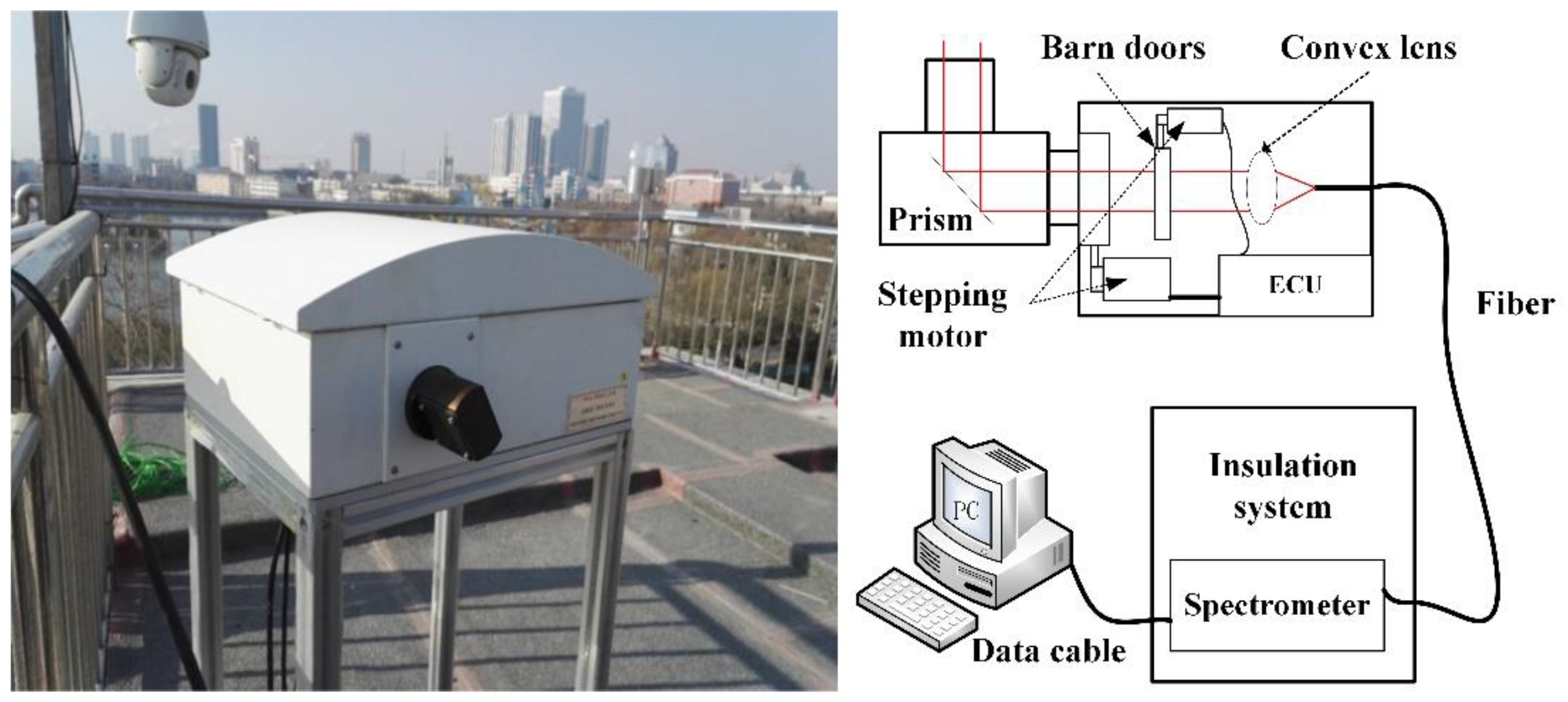
2.2. Ground-Based MAX-DOAS Data

The same MAX-DOAS measurement system deployed in the NCP has also been used to retrieve the tropospheric columns and vertical distributions of trace gases such as NO₂ and formaldehyde, and to quantify the pollution at a certain point [45]; this system was manufactured by the Anhui Institute of Optics and Fine Mechanics, China. The system is mainly composed of a spectrum acquisition module and a data processing module (Figure 2). It uses a stepping motor to control the steering of the lens collecting the spectrum at elevation angles of 5, 15, 30, 60, and 90, and measures the NO₂ amounts on different optical paths. A full collection cycle requires approximately 5–15 min owing to the automatic integral time.

We used the zenith measurement spectrum recorded at noon locally as the reference spectrum to obtain the NO₂ differential slant column density (DSCD), which significantly minimized the interference from the stratospheric atmosphere on the tropospheric measurements. The best fitting wavelength intervals and the absorption cross-sections considered are described in Table 1. Then, by using the DSCD of different angles to obtain the local NO₂ profile, we combined the differential air mass factor (dAMF) hold by the radiation transfer model to obtain the tropospheric NO₂ VCDs.

Table 2. Details of the MAX-DOAS ground-based sampling locations in the North China Plain (NCP).

Sites	Coordinates	Spectral Resolution	Observation Date	Azimuth
Beijing	116.32° E, 39.95° N	0.6 nm	01.11.2018–30.04.2019	0°
Tianjin	117.29° E, 39.69° N	0.6 nm	01.11.2018–30.04.2019	355°
Baoding	115.514° E, 38.865° N	0.3 nm	01.11.2018–09.03.2019 14.04.2019–30.04.2019	18°
Cangzhou	116.86° E, 38.31° N	0.5 nm	01.11.2018–16.03.2019 02.04.2019–30.04.2019	19°

shows the details of the four ground-based MAX-DOAS sites in the BTH region. Due to the need for daily maintenance (calibration) of the spectrometer, data on certain days were missing. In addition, the observation azimuth of the telescope was taken into account to prevent direct sunlight and building blockages.

As the DOAS observation system uses scattered sunlight as the light source for spectral detection, cloudy or foggy weather significantly decreases the accuracy of the NO₂ inversion [46]. Therefore, all data mentioned in this study from the EMI and ground-based sensors were selected only on days when the satellite passed the ground station and the relative cloud cover was less than 0.5. The relative cloud cover was characterized by the cloud reflectivity obtained from EMI radiance products [47].

2.3. Auxiliary Data

When analyzing the pollution distribution, it is necessary to consider the influence of atmospheric transport. In this study, wind speed and wind direction data were extracted from the Copernicus Atmosphere Monitoring Service (CAMS) reanalysis data [48]. The smog levels were provided by the State Environmental Protection Administration (EPA) to screen NO₂ data from the EMI and ground-based MAX-DOAS observations in the NCP (http://www.pm25.in/, accessed on 19 March 2021).

2.4. Methodology

A direct comparison of the trend in NO₂ observed by the EMI and MAX-DOAS will cause the results with large differences to not be directly reflected in the correlation. Therefore, this study analyzed the results of the mean difference (Equation (1)) and mean relative difference (Equation (2)) of NO₂ VCD:

$$\mathrm{MD}=\frac{1}{n}{\displaystyle \sum }_{i=1}^n\left({\mathrm{VCD}}_{max-doas, i}-{\mathrm{VCD}}_{EMI, i}\right)$$

(1)

$$\mathrm{MRD}=\frac{1}{n}{\displaystyle \sum }_{i=1}^n\left(\frac{{\mathrm{VCD}}_{max-doas,i}-{\mathrm{VCD}}_{EMI,i}}{{\mathrm{VCD}}_{max-doas,i}}\right)\times 100\%$$

(2)

where $\mathrm{MD}$ is the mean absolute difference, and $\mathrm{MRD}$ is the mean relative difference. A positive (negative) $\mathrm{MD}$ is thus an indication of EMI overestimation (underestimation), and a small (large) $\mathrm{MRD}$ value reflects high (low) agreement between the EMI and the ground-based observation results. Additionally, the Pearson correlation coefficient and fitting slope were used to validate the results and to explain the correspondence between the EMI NO₂ vertical column densities and the corresponding averages from the ground-based MAX-DOAS measurements.

In the analysis of the impact of the wind field on pollution change in the NCP region using EMI data products, a combination of cluster analysis and two-way analysis of variance (ANOVA) was performed [49]. Because different daily wind speeds and directions might easily cause large degrees of freedom as independent variables, the wind speed, as a meteorological factor, was rounded according to the actual wind speed, and the wind direction data were divided into 16 clusters based on the direction of 22.5°. Finally, taking the NO₂ column as the dependent variable, a two-way analysis of variance was used to quantitatively analyze the NO₂ changes.

3. Results

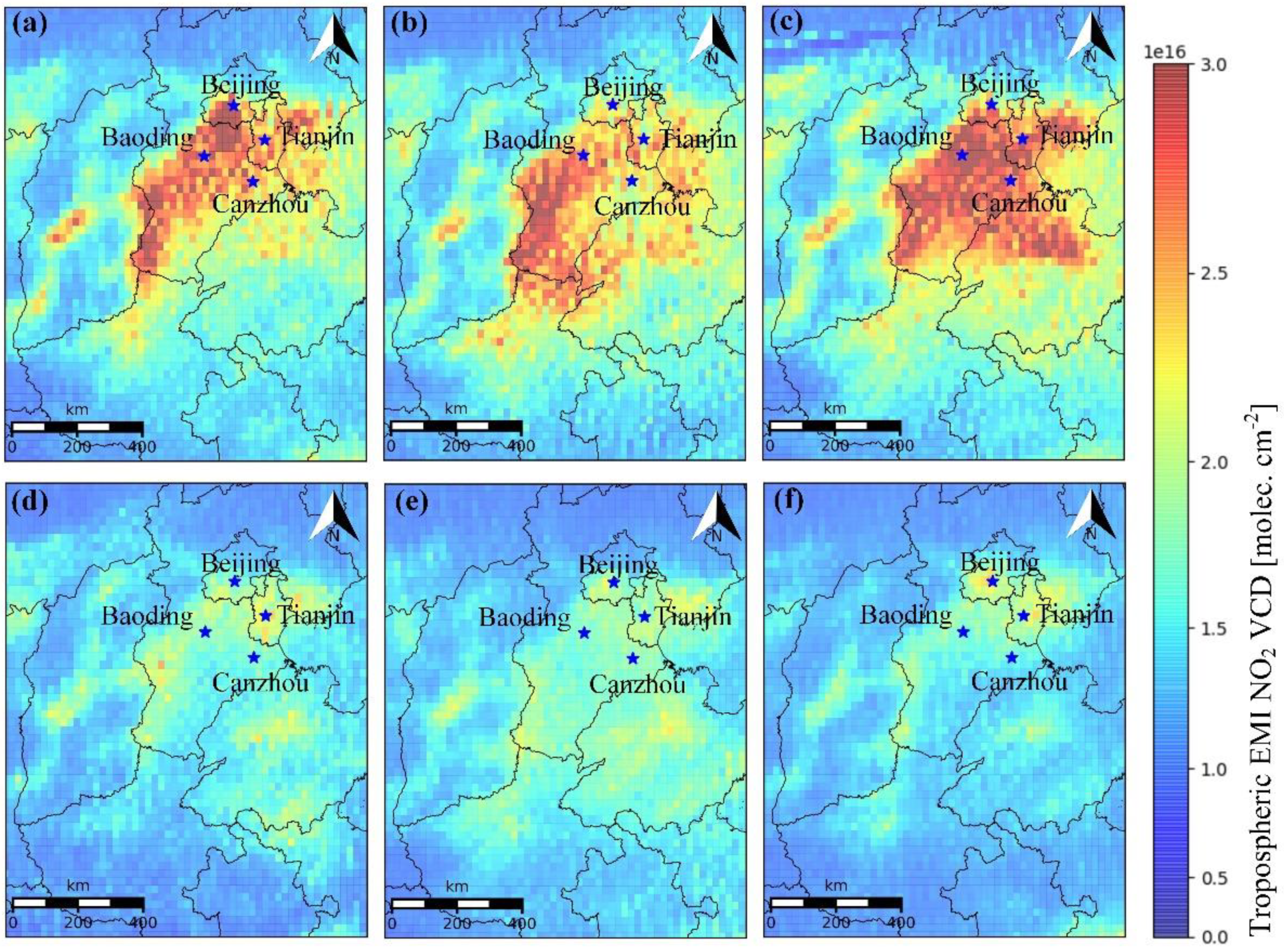
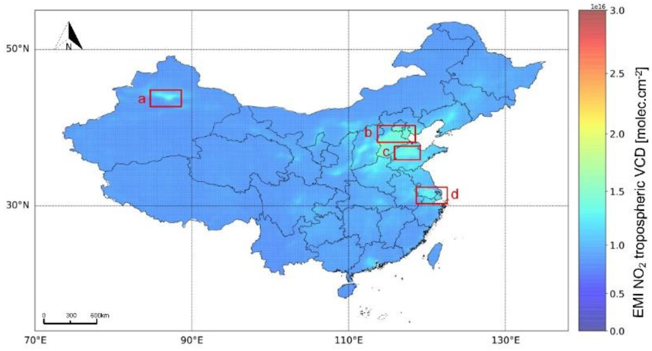
3.1. Spatial Distribution of Tropospheric NO₂ in the NCP

The average distribution of the NO₂ VCD in the troposphere of mainland China from November 2018 to April 2019 was measured via spectrum inversion using EMI data (Figure 3). The NO₂ distribution in China was uneven. For example, some economically developed regions such as Urumqi (Figure 3a), Beijing–Tianjin–Hebei (BTH) (Figure 3b), central Shandong (Figure 3c), and Yangtze River Delta (Figure 3d) showed relatively high NO₂ column amount in the troposphere. NO₂ pollution in the winter in North China was quite distinct, particularly because of the fossil fuel used for heating purposes.

A detailed assessment of NO₂ pollution also is useful for local-scale analyses to better evaluate the role of pollution sources and pollution changes. For these purposes, NO₂ pollution in the NCP (32° N–42° N, 110° E–120° E), where the capital city of China is located, was analyzed in detail (Figure 4).

The NO₂ distribution maps from November 2018 to January 2019 (Figure 4a–c) revealed that the level of pollution could persist for a couple of months over large areas across the NCP. This period corresponded to the normal conditions of economic activities and winter heating in northern China, which are characteristic of a region with a dense population.

As a result of increases in temperature, NO₂ levels decreased considerably from February to April (Figure 4d–f), which resulted in an improvement of the air quality. In addition, the high NO₂ distribution in the NCP showed considerable reductions in terms of the spatial extent, and only some megalopolis hotspots and isolated hotspots with heavy industries remained.

The spatial coverage areas and changes in NO₂ clearly indicated that most parts of the NCP are subjected to air pollution in the winter. The highest NO₂ mainly appeared in the southern part of Beijing, in most of Tianjin, in the central and south parts of Hebei, and in northeast Shandong, where the tropospheric NO₂ column density maintained high values of over 3 × 10¹⁶ molecules cm⁻². These results indicate that when a large area of pollution recedes, some hot spots of pollution will remain, which can be attributed to vehicle traffic and intensive industrial activities. However, the highest monthly mean NO₂ VCD was found to be less than 2.5 × 10¹⁶ molecules cm⁻².

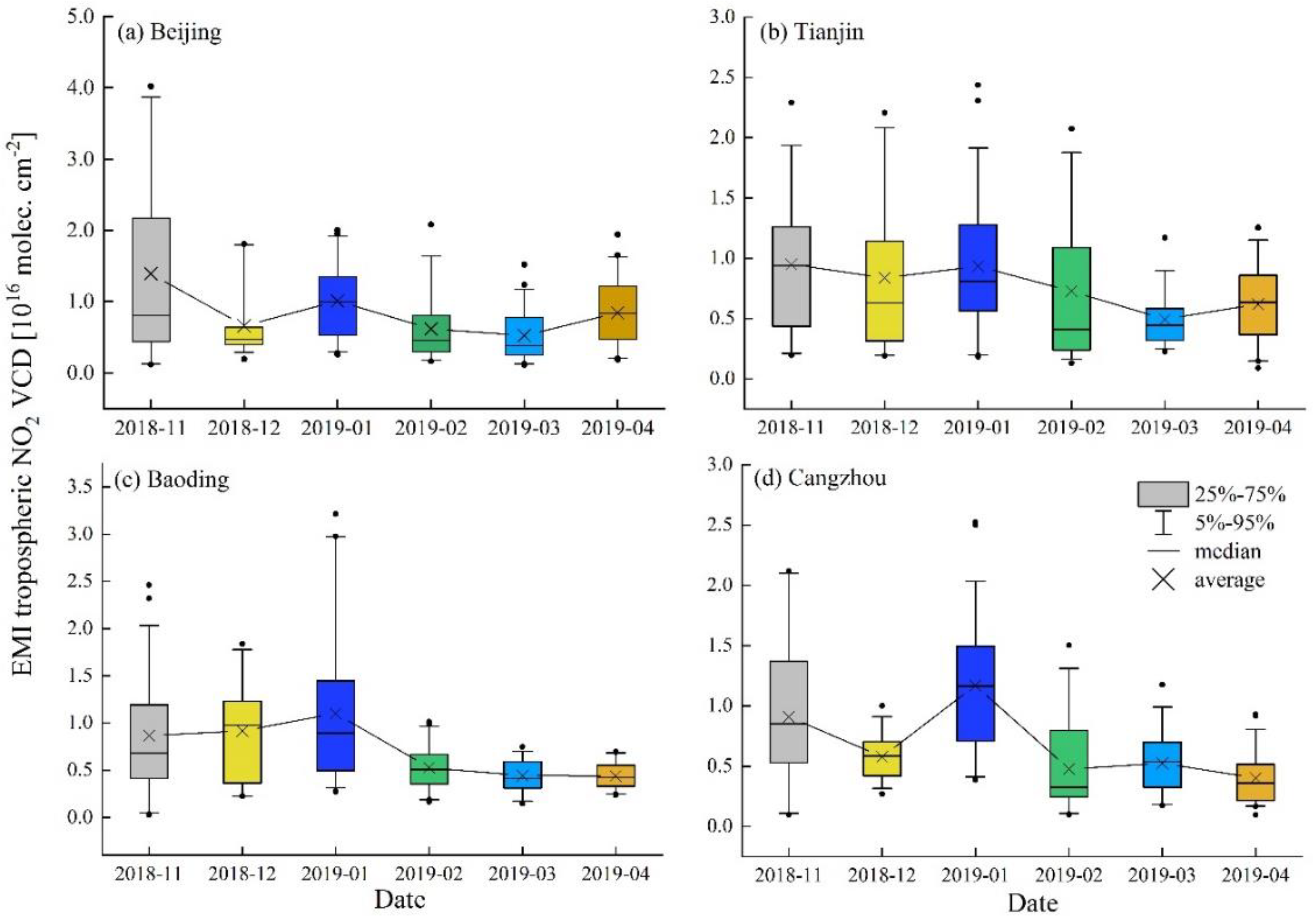
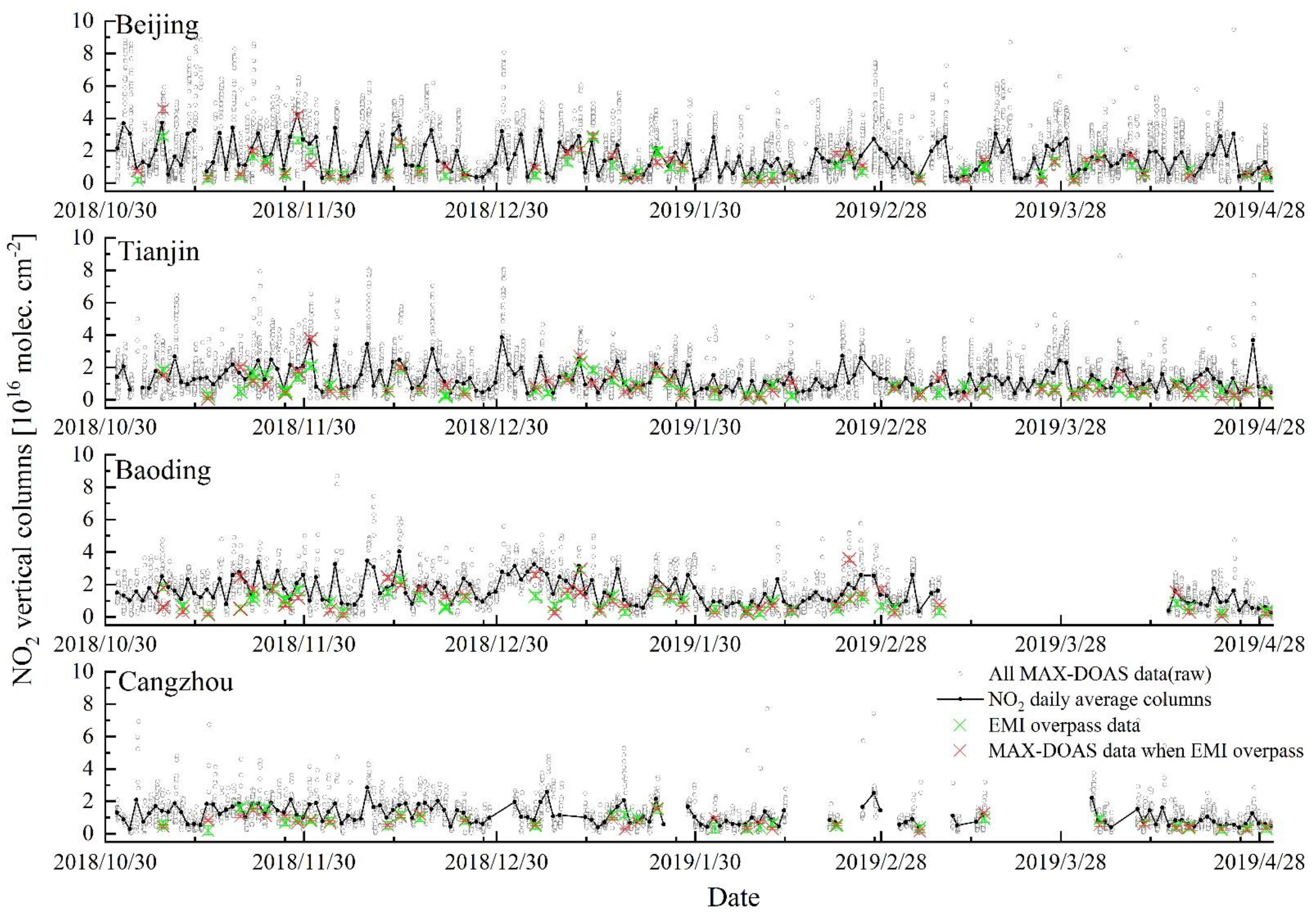
3.2. Monthly Averaged NO₂ Columns of the Four Main Cities

The monthly average columns of NO₂ monitored by the EMI for the region within a 0.15 latitude and longitude (~16.7 km × 13 km in the NCP) distance of the four ground stations (Beijing, Baoding, Cangzhou, and Tianjin city) are illustrated in Figure 5.

Temporal variations in data were observed in the EMI NO₂ datasets. High NO₂ pollution levels were found during winter in the four urban regions. However, the months in which the mean NO₂ columns were highest in different regions varied. This variation was likely related to the meteorological conditions (e.g., monsoons) and economic activity. The anomalous high points in Figure 5 represent high values of the tropospheric NO₂ VCD, which correspond to the most polluted days for the analyzed period. In contrast, the outlier points for the lower points may correspond to weather parameters that favored pollution reductions, such as a particular wind regime or rain wash-out.

4. Discussion

4.1. Error Analysis

The uncertainty of tropospheric NO₂ inversion mainly includes two parts: (a) the uncertainty of inversion of SCD, (b) the uncertainty of AMF in the VCD calculation. For EMI NO₂ observations, as it involves the separation of NO₂ columns in the stratosphere and troposphere, the NO₂ VCD inversion in the troposphere of the spaceborne platform also includes stratosphere–troposphere separation error. Assuming that these uncertainties are independent, the total uncertainty of the tropospheric NO₂ VCD for MAX-DOAS and EMI can be quantified as follows:

$${\mathsf{\epsilon }}_{\max -\mathrm{doas}}=\sqrt{{\left(\frac{{\sigma }_{\mathrm{DSCD}}}{d\mathrm{AMF}}\right)}^2+{\left(\frac{\mathrm{DSCD}}{d{\mathrm{AMF}}^2}\times {\sigma }_{d\mathrm{AMF}}\right)}^2}$$

(3)

$${\mathsf{\epsilon }}_{\mathrm{EMI}}=\sqrt{{\left(\frac{{\sigma }_{\mathrm{SCD}}{}_{\mathrm{total}}}{\mathrm{AMF}}\right)}^2+{\left(\frac{{\sigma }_{\mathrm{SCD}}{}_{\mathrm{strat}}}{\mathrm{AMF}}\right)}^2+{\left(\frac{{\mathrm{SCD}}_{\mathrm{total}}-{\mathrm{SCD}}_{\mathrm{strat}}}{{\mathrm{AMF}}^2}\times {\sigma }_{\mathrm{AMF}}\right)}^2}$$

(4)

With ${\sigma }_{\mathrm{DSCD}}$, ${\sigma }_{\mathrm{SCD}}{}_{\mathrm{total}}$, and ${\sigma }_{\mathrm{SCD}}{}_{\mathrm{strat}}$ the slant column error ${\sigma }_{\mathrm{AMF}}$, ${\sigma }_{\mathrm{dAMF}}$ are the error of tropospheric AMF based on EMI and the difference AMF estimation error of ground-based MAX-DOAS, respectively.

For ${\sigma }_{\mathrm{DSCD}}$, ${\sigma }_{\mathrm{SCD}}{}_{\mathrm{total}}$, originate from the DOAS fitting residuals, which can be obtained directly in the spectral fitting. This uncertainty is mainly dominated by the instrument noise, and other systematic errors, such as the uncertainty of fitting the absorption cross-sections and the uncertainty of spectral correction. In this study, the mean vertical errors of fitting MAX-DOAS for Beijing, Tianjin, Baoding, and Cangzhou foundations during the observation period were 1.1 × 10¹⁵ molecules cm⁻², 9.2 × 10¹⁴ molecules cm⁻², 1.2 × 10¹⁵ molecules cm⁻², and 8.6 × 10¹⁴ molecules cm⁻², respectively. ${\sigma }_{\mathrm{SCD}}{}_{\mathrm{strat}}$ is stratospheric slant column error. Because this study uses RSM to separate the NO₂ columns in the stratosphere and the troposphere, this part of the error is related to the RSM 7.6 × 10¹⁴ molecules cm⁻² [50].

The tropospheric AMF and dAMF were calculated by the radiation transfer model, and depend on a priori gas profile and model parameters (cloud cover, surface reflectivity, etc.). In addition, AMF is also related to the geometric parameters such as the solar zenith angle, the relative azimuth angle and the viewing zenith angle, but the measurement geometry is known with high accuracy and therefore does not contribute significantly to the AMF errors. Therefore, ${\sigma }_{\mathrm{AMF}}$, ${\sigma }_{d\mathrm{AMF}}$ mainly depends on the surface albedo, NO₂ profile, aerosol and cloud cover.

In the comparative study, the NO₂ data of MAX-DOAS and EMI were selected according to cloud cover, and the contribution of cloud cover can be ignored. In addition, most of the input parameters in the AMF simulation come from the chemical transfer model and the weather website, errors will be dampened to some extent. For the impact of the NO₂ profile on AMF, the NO₂ profile in the 2 × 2.5° geographic grid simulated by the GEOS-Chem model was used as the input parameter of the radiation transfer model, then, simulate the maximum standard deviation of the AMF as the error introduced by the difference in NO₂ profile. In the same way, the perturbation error of the surface albedo to the AMF is also based on the same calculation method. Different types of aerosols and the altitude of the aerosol layer have different assessments of AMF. In the calculation of AMF, the aerosol optical thickness was assumed to be 0.06. To evaluate the influence of different aerosol scenarios on the AMF under spaceborne and ground-based observation, the actual daily average aerosol data product (https://aeronet.gsfc.nasa.gov/, accessed on 19 March 2021) was used as the input parameter of the radiation transfer model to simulate AMF. The results show that, during the observation period, the influence of aerosols on the AMF of the spaceborne and ground-based observation methods is 0.02% and 0.2%, respectively.

The results in

Table 3. Error in the retrieval of tropospheric vertical NO₂ column from EMI and MAX-DOAS (10¹⁵ molecules cm⁻²).

		Beijing		Tianjin		Baoding		Cangzhou
		MAX-DOAS	EMI	MAX-DOAS	EMI	MAX-DOAS	EMI	MAX-DOAS	EMI
Fitting error, ${\sigma }_{\mathrm{SCD}}/d\mathrm{AMF}$ or ${\sigma }_{\mathrm{DSCD}}/d\mathrm{AMF}$		1.1	0.92	0.92	1.01	1.2	0.91	0.86	0.9
stratosphere–troposphere separation error, ${\sigma }_{{\mathrm{SCD}}_{\mathrm{strat}}}/\mathrm{AMF}$		-	0.76	-	0.76	-	0.76	-	0.76
AMF error, ${\sigma }_{\mathrm{AMF}}$, ${\sigma }_{\mathrm{dAMF}}$	surface albedo	0.23	0.39	0.16	0.32	0.27	0.41	0.2	0.34
	NO2 profile	0.17	0.2	0.12	0.17	0.19	0.2	0.14	0.15
	aerosol	0.002	0.02	0.015	0.002	0.02	0.002	0.014	0.002
Total error		1.1	1.3	0.9	1.3	1.2	1.3	0.9	1.2

provide a general estimate of overall retrieval uncertainties that may be expected for tropospheric NO₂ data under different conditions.

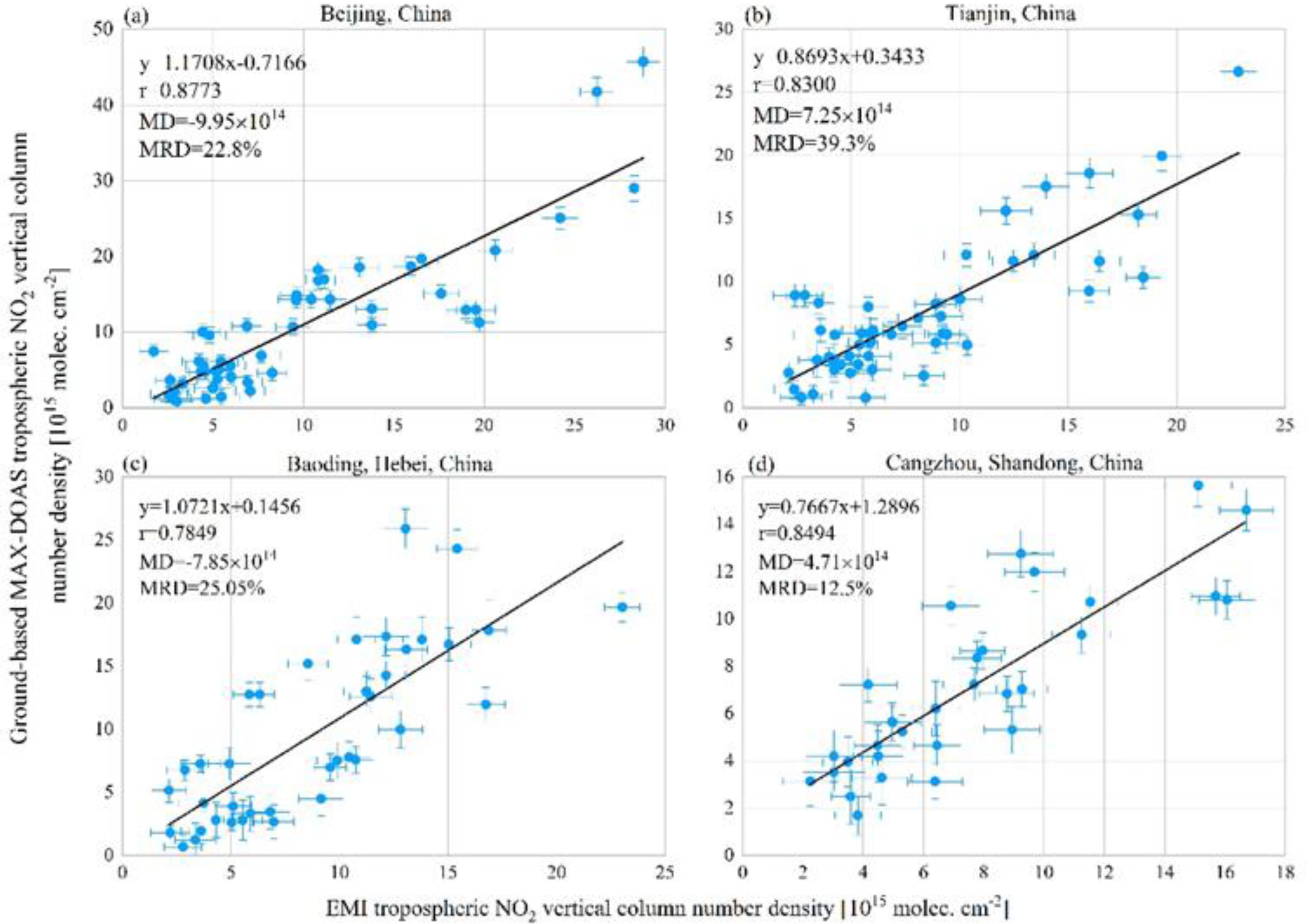
4.2. Comparison of EMI and Ground-Based MAX-DOAS Observations

The comparison of the tropospheric NO₂ between the EMI and MAX-DOAS data provided useful information about the changes in NO₂ within the NCP. Figure 6 shows the time series of the tropospheric NO₂ VCD variations derived from the EMI and MAX-DOAS in four cities, and these data cover the period from November 2018 to April 2019. The MAX-DOAS NO₂ vertical columns are shown in their original time resolution (gray dots) as well as averaged 60 min around the EMI overpass (red star points) for all cloud-free days (EMI cloud fraction ≤ 0.5). The latter were used in the comparison for the EMI NO₂ tropospheric vertical columns (green star points). Only the NO₂ results of the cloud-screened quality-controlled data meeting the conditions were considered for the comparison.

Through the comparison of the EMI and MAX-DOAS measurements, it was observed that the collocated vertical columns mostly followed the same day-to-day variability. We noted that slight differences occurred between the EMI and ground-based vertical columns, in which the MAX-DOAS results were larger than the EMI results in some cases but not in others, and these findings correspond to the fact that the results did not match perfectly for the EMI and MAX-DOAS measurements. This was expected because of the influence of cloud cover and smog, as well as the differences in spatial representation; in addition, the greater period averaging of ground-based data within 60 min compared to the EMI overpass sampling time could have contributed to the differences.

The EMI tropospheric NO₂ column was statistically compared with datasets derived from MAX-DOAS NO₂ columns from selected potential sources of pollution or contaminated areas. The validation results showed that there was a high correlation between ground-based and satellite-based data for the selected sites during half of a year. Specifically, the correlation coefficients were 0.88, 0.83, 0.78, and 0.85 for Beijing, Tianjin, Baoding, and Cangzhou, respectively, as shown in Figure 7. Moreover, the MD values were positive in Tianjin and Cangzhou, which means that, on average, the EMI slightly overestimated the NO₂ columns in comparison with the ground-based data in Tianjin and Cangzhou. Correspondingly, the MD values for Beijing and Baoding were negative, as the EMI products underestimated the data in Beijing and Baoding in comparison with the ground-based products. When considering the MRD for the four datasets, the biases were all positive and the values were not large, but variations remained within the uncertainties.

In fact, according to some other satellite-based and ground-based NO₂ product comparisons, the correlation values can be high between the EMI and ground-based MAX-DOAS NO₂ observations. For instance, the NO₂ columns derived by MAX-DOAS installed at the Royal Meteorological Institute, Brussels, were used to analyze the correlation with Tropomi products, classified according to seasons, and the correlation between the two datasets reached up to 0.85, while the average value was around 0.7 [51]. Meanwhile, the correlation between the OMI and ground-based MAX-DOAS data was found to be relatively low, with the correlation coefficients in the Mohali area between 0.38 and 0.56 [52].

Overall, the EMI, a state-of-the-art hyperspectral remote sensing instrument of China, can grasp the distribution of NO₂, and EMI products can play an important role in the analyses of trace gases and the daily variation trends of pollution on a large scale. Meanwhile, ground-based MAX-DOAS measurements have high temporal resolutions, which is of great significance for analyzing the daily and monthly changes of local pollutants.

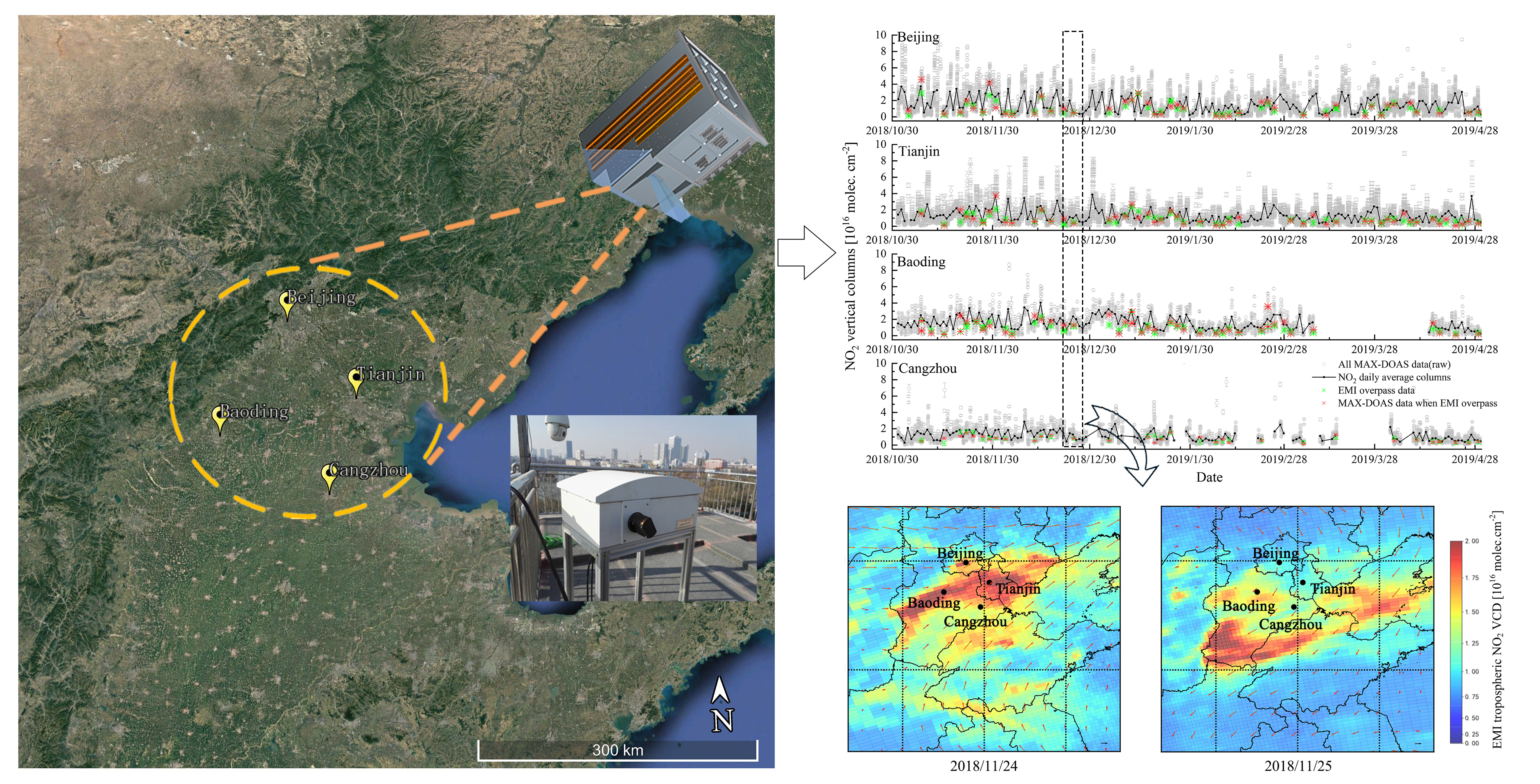
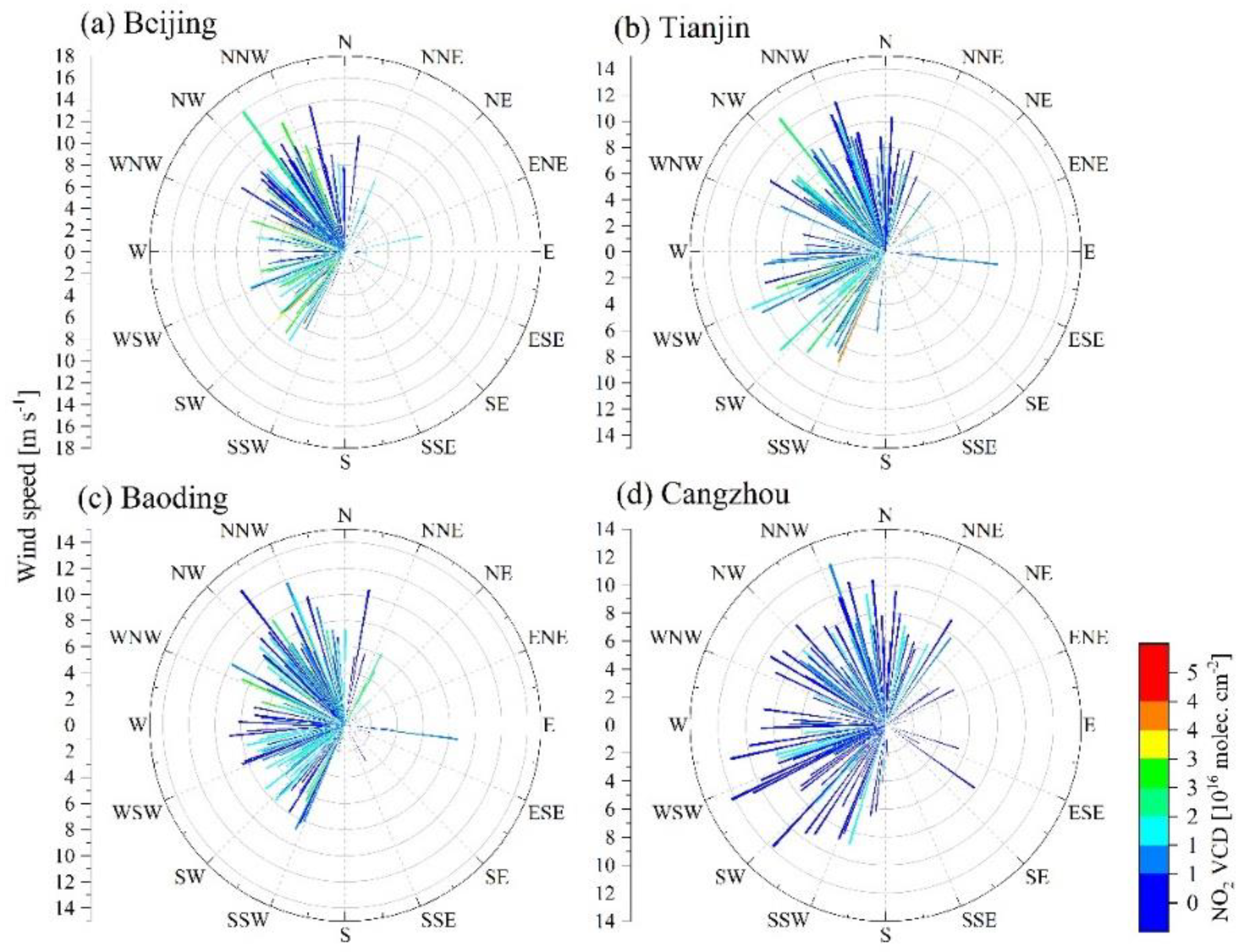
4.3. Application of EMI to NO₂ Pollution Transfer Monitoring

As mentioned in Section 3.1, during winter, the NO₂ amounts in North China are significantly elevated. For the analysis of the tropospheric NO₂ pollution process in the NCP, we considered the following three main factors: the emission of nitrogen oxides, the lifetime of NOx, and the meteorological conditions. First, NOx is produced through coal burning. During winter, heating in the north corresponds to increased coal consumption. Second, due to the low temperatures in winter, the lifetime of NOx is longer than that in other seasons, which delays the progression of atmospheric chemical reactions, slows down the degradation rate of NO₂, and causes NO₂ build-up in the atmosphere. Finally, worsening meteorological conditions in winter accelerate pollution. Driven by the effects of lower temperatures, the atmospheric boundary layer is lower in winter, and thus, most of the NO₂ remains in the lower troposphere.

In this study, the correlation between the wind field and NO₂ changes was analyzed. The wind field is an important factor leading to NO₂ changes. Under the influence of the winter monsoon, NO₂ can be transported over long distances, which can lead to severe NO₂ pollution events even in areas with few local industrial activities in the NCP. The impact of the wind pattern on NO₂ pollution in the NCP area was analyzed in detail. Statistical methods were used to reveal the sources of pollutant transport at each site. Figure 8 shows the statistical wind rose diagrams between the wind fields and NO₂ columns in Beijing, Tianjin, Baoding, and Cangzhou from November 2018 to April 2019. The direction of the wind field in the rose diagram denotes the real wind direction. Different colored bars represent the daily maximum column of NO₂ measured by MAX-DOAS.

The statistical results illustrate the correlations between the NO₂ transport and the wind field. According to wind field statistics, these four regions are less exposed to easterly weather in winter. When the wind direction was southwest, which is an important transport route, the NO₂ column amount showed a higher value than that for the other wind directions in Beijing and Tianjin. However, the results indicated that the correlation between NO₂ and the wind field was weak in Cangzhou.

To analyze the influence of wind directions on NO₂ pollution, a two-way analysis of variance was adopted. The variation of NO₂ only under the effects of different wind speeds and wind directions was explained. The wind direction was treated as the independent variable and wind speed as the covariate.

Table 4. Two-way analysis of variance of wind fields in Beijing, Tianjin, Cangzhou, and Baoding.

Sites		Wind Speed	Wind Direction	Levene Test 1
Beijing	F	0.005	2.348	1.669
	p	0.944	0.007	0.072
Tianjin	F	2.708	2.044	1.587
	p	0.102	0.02	0.093
Baoding	F	6.309	1.215	1.373
	p	0.013	0.272	0.175
Cangzhou	F	9.172	0.003	2.274
	p	1.379	0.169	0.001

¹ When the p value of the Levene test was greater than 0.05, this meant that the samples had an equal variance. A p value of ≤0.05 was considered to be of statistical significance for a single factor.

shows the results for the two-way analysis of variance of wind fields in Beijing, Tianjin, Baoding, and Cangzhou based on the wind direction and wind speed. By comparing the p value of the respective variables at a level of 0.05, the statistical analysis revealed that the wind direction had a significant impact on the NO₂ columns in Beijing and Tianjin.

The marginal mean of the main effect based on the analysis of variance was computed. The results showed that when the wind direction was approximately 22.5–45 degrees south by west, the maximum marginal mean columns of NO₂ was 8.647 × 10¹⁶ molecules cm⁻². That is, the wind field with this wind direction had the most apparent influence on the NO₂ changes in Beijing. Likewise, the correlation between the change in NO₂ and wind direction was also obvious in Tianjin. However, no apparent evidence that the NO₂ changes have a high correlation with the wind field was found in Baoding and Cangzhou, which indicates that local emissions rather than transport are the most important sources of NO₂ pollution in these two regions.

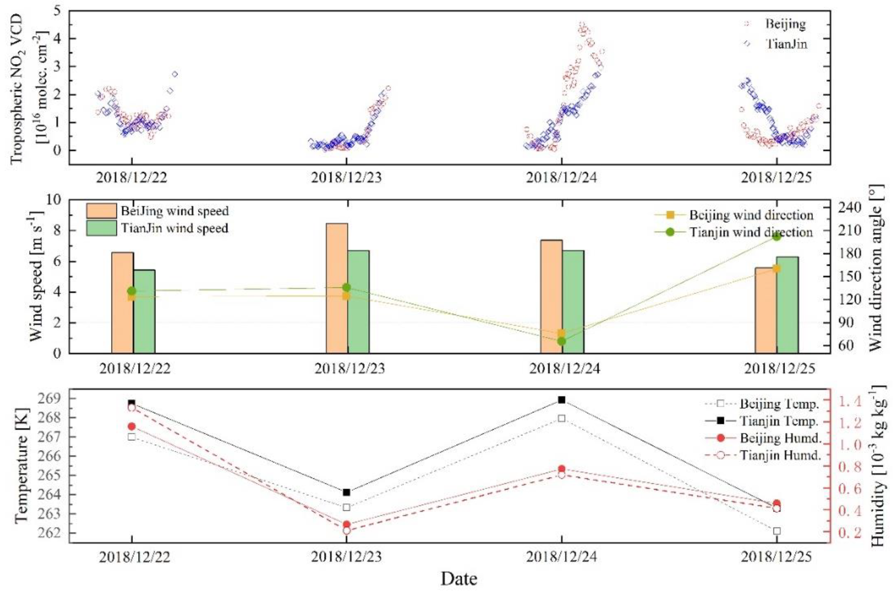
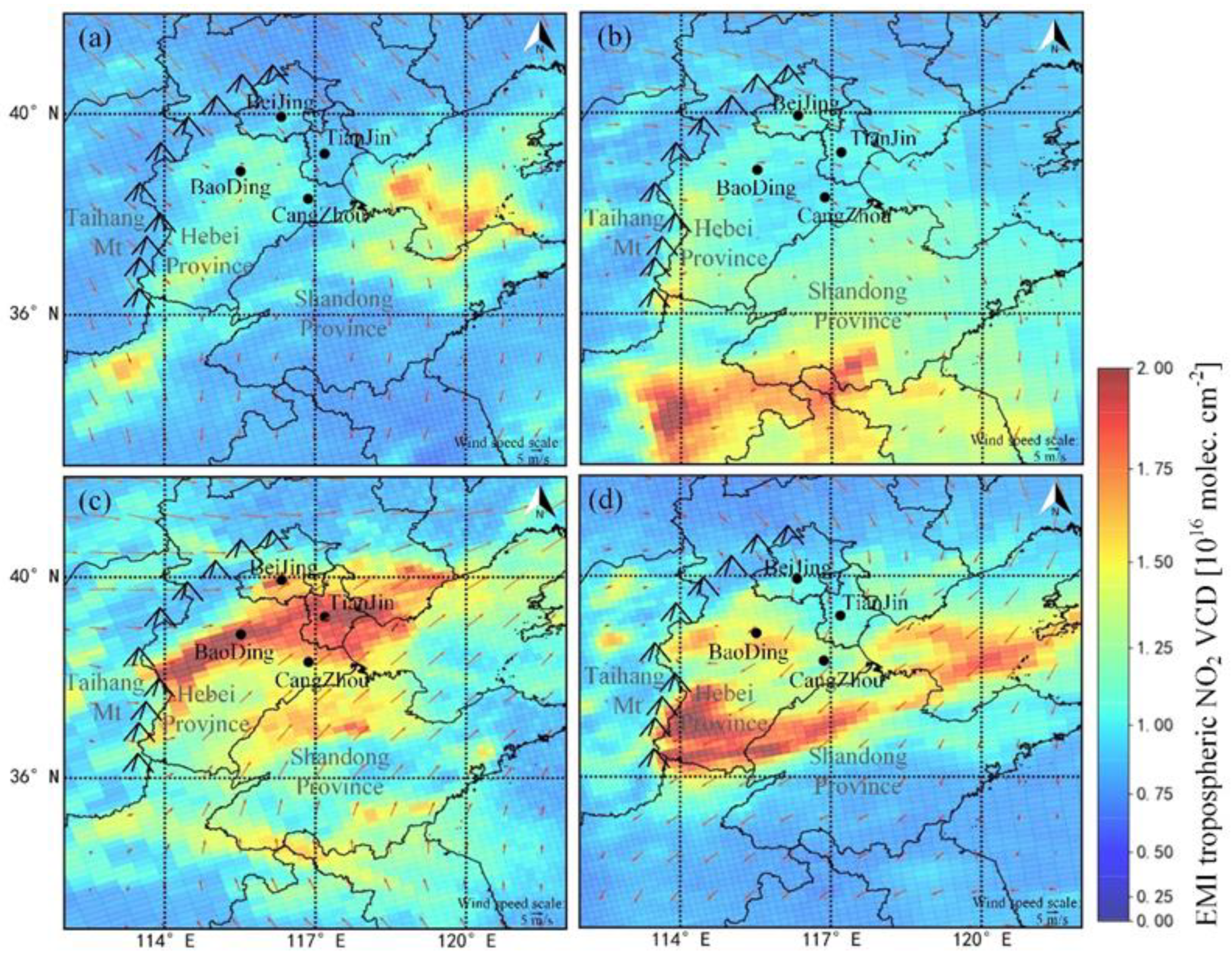
4.4. Local Scale NO₂ Pollution Mapping and Pollution Transport: A Case Study of Beijing and Tianjin

For Beijing and Tianjin, the influence of wind fields on the NO₂ changes in December 2018 was determined by analyzing the NO₂ column amounts and meteorological conditions, including the temperature, humidity, wind speed, and direction at 850 hPa atmospheric pressure.

As mentioned before, high-pollution episodes occur frequently in Beijing and Tianjin in December. Figure 9 shows a time series diagram of the NO₂ changes retrieved by MAX-DOAS and the meteorological conditions at the Beijing and Tianjin sites during 22–25 December 2018. The NO₂ columns exhibited an obvious variation trend. The change process was strongly associated with the wind direction, that is, when the wind direction was a southeast wind, NO₂ showed an increasing trend.

The EMI NO₂ products also showed good capture of the pollution process. Figure 10 shows the NO₂ distribution map and the wind field of the NCP during 22–25 December 2018. The aggregation of NO₂ was obvious in Beijing when the wind field was a southwest wind, and this area is surrounded by the Taihang Mountains in the north and west. However, results showed that when the wind field was northwest, there was no obvious pollution transportation from the northeast direction of Beijing. Meanwhile, the NO₂ columns measured by the EMI in Beijing and Tianjin were low on those days. Wind fields and NO₂ variation reveal a potential pollution transport channel in the southwest direction of Beijing and Tianjin.

5. Conclusions

In recent years, the Chinese government has put forth significant efforts toward energy conservation and emission reductions. In this respect, the 12th and 13th Five-Year Plans have been formulated to reduce the impacts of air pollution such as that caused by nitrogen oxides and other greenhouse gases on ecosystems and the environment. However, during particular months, heavy NO₂ pollution can still be observed in some areas. Therefore, NO₂ pollution monitoring is an important task for identifying emissions and developing effective reduction strategies.

The recently launched Environmental Trace Gases Monitoring Instrument (EMI) payload on the GF-5 satellite allows for the monitoring of trace gases, and these data can be used to analyze atmospheric pollution on different scales from large cities to global coverage. In this study, we used the new satellite EMI payload to observe the NO₂ amounts in North China from November 2018 to April 2019, in combination with ground-based multi-axis differential optical absorption spectroscopy (MAX-DOAS) observation data and numerical models. The main conclusions can be summarized as follows:

(a) Using six months’ worth of data over the North China Plain (NCP), the correlation coefficient of tropospheric NO₂ between the EMI and MAX-DOAS located at four sites reached 0.88. The spatial distribution and changes in tropospheric NO₂ of EMI agreed well with ground-based observations. The good agreement of NO₂ products shows that the EMI can be used to accurately monitor tropospheric NO₂ pollution.

(b) The distribution of NO₂ in China showed obvious temporal and spatial variation, in which higher amounts of pollution were detected in winter. The NO₂ in the NCP from November to January increased owing to the large quantities of fossil fuel consumption in North China for heating.

(c) Based on observations and statistical analysis, the wind field is one of the important factors affecting the distribution of NO₂ pollution in the NCP region. The southwest wind in Beijing and Tianjin has a correlation with the increase of NO₂ to a certain degree.

This research is a good demonstration of how a comprehensive understanding of regional NO₂ pollution can be obtained through joint observations of the EMI and ground-based MAX-DOAS, and this technique will be applied to more research projects in the future.

References

1. Levine, S.Z.; Uselman, W.M.; Chan, W.H.; Calvert, J.G.; Shaw, J.H. The kinetics and mechanisms of the HO2-NO2 reactions; the significance of peroxynitric acid formation in photochemical smog. Chem. Phys. Lett. 1977, 48, 528–535. [Google Scholar] [CrossRef]
2. Ma, J.; Xu, X.; Zhao, C.; Yan, P. A review of atmospheric chemistry research in China: Photochemical smog, haze pollution, and gas-aerosol interactions. Adv. Atmos. Sci. 2012, 29, 1006–1026. [Google Scholar] [CrossRef]
3. Zhang, G.Z.; Liu, D.Y.; He, X.H.; Yu, D.Y.; Pu, M.J. Acid rain in Jiangsu province, eastern China: Tempo-spatial variations features and analysis. Atmos. Pollut. Res. 2017, 8, 1031–1043. [Google Scholar] [CrossRef]
4. Katsouyanni, K. Ambient air pollution and health. Br. Med. Bull. 2003, 68, 143–156. [Google Scholar] [CrossRef] [Green Version]
5. Itano, Y.; Bandow, H.; Takenaka, N.; Saitoh, Y.; Asayama, A.; Fukuyama, J. Impact of NOx reduction on long-term ozone trends in an urban atmosphere. Sci. Total Environ. 2007, 379, 46–55. [Google Scholar] [CrossRef] [PubMed]
6. Chen, B.; Kan, H. Air pollution and population health: A global challenge. Environ. Health Prev. Med. 2008, 13, 94–101. [Google Scholar] [CrossRef] [PubMed] [Green Version]
7. Van der, A.R.J.; Eskes, H.J.; Boersma, K.F.; Van Noije, T.P.C.; Van Roozendael, M.; De Smedt, I.; Peters, D.H.M.U.; Meijer, E. Trends, seasonal variability and dominant NOx source derived from a ten year record of NO2 measured from space. J. Geophys. Res. 2008, 113, D04302. [Google Scholar] [CrossRef]
8. Al-Harbi, M.; Al-majed, A.; Abahussain, A. Spatiotemporal variations and source apportionment of NOx, SO2, and O3 emissions around heavily industrial locality. Environ. Eng. Res. 2020, 25, 147–162. [Google Scholar] [CrossRef]
9. Li, J.F.; Wang, Y.H. Inferring the anthropogenic NOx emission trend over the United States during 2003–2017 from satellite observations: Was there a flattening of the emission trend after the Great Recession? Atmos. Chem. Phys. 2019, 19, 15339–15352. [Google Scholar] [CrossRef] [Green Version]
10. Haridas, M.K.M.; Gharai, B.; Jose, S.; Prajesh, T. Multi-year satellite observations of tropospheric NO2 concentrations over the Indian region. J. Earth Syst. Sci. 2019, 128, 9. [Google Scholar] [CrossRef] [Green Version]
11. Sun, W.; Shao, M.; Granier, C.; Liu, Y.; Ye, C.S.; Zheng, J.Y. Long-Term Trends of Anthropogenic SO2, NOx, CO, and NMVOCs Emissions in China. Earth Future 2018, 6, 1112–1133. [Google Scholar] [CrossRef] [Green Version]
12. Zhang, X.Y.; Zhang, P.; Zhang, Y.; Li, X.J.; Qiu, H. The trend, seasonal cycle, and sources of tropospheric NO2 over China during 1997-2006 based on satellite measurement. Sci. China Ser. D Earth Sci. 2007, 50, 1877–1884. [Google Scholar] [CrossRef]
13. Rohde, R.A.; Muller, R.A. Air Pollution in China: Mapping of Concentrations and Sources. PLoS ONE 2015, 10, e0135749. [Google Scholar] [CrossRef]
14. Wang, C.; Wang, T.; Wang, P.; Rakitin, V. Comparison and Validation of TROPOMI and OMI NO2 Observations over China. Atmosphere 2020, 11, 636. [Google Scholar] [CrossRef]
15. Xue, R.B.; Wang, S.S.; Li, D.R.; Zou, Z.; Chan, K.L.; Valks, P.; Saiz-Lopez, A.; Zhou, B. Spatio-temporal variations in NO2 and SO2 over Shanghai and Chongming Eco-Island measured by Ozone Monitoring Instrument (OMI) during 2008-2017. J. Clean. Prod. 2020, 258, 120563. [Google Scholar] [CrossRef]
16. Gu, D.; Wang, Y.; Smeltzer, C.; Boersma, K.F. Anthropogenic emissions of NOx over China: Reconciling the difference of inverse modeling results using GOME-2 and OMI measurements. J. Geophys. Res. 2014, 119, 7732–7740. [Google Scholar] [CrossRef]
17. Liu, F.; Page, A.; Strode, S.A.; Yoshida, Y.; Choi, S.; Zheng, B.; Lamsal, L.N.; Li, C.; Krotkov, N.A.; Eskes, H.; et al. Abrupt decline in tropospheric nitrogen dioxide over China after the outbreak of COVID-19. Sci. Adv. 2020, 6, eabc2992. [Google Scholar] [CrossRef]
18. Pei, Z.; Han, G.; Ma, X.; Su, H.; Gong, W. Response of major air pollutants to COVID-19 lockdowns in China. Sci. Total Environ. 2020, 743, 140879. [Google Scholar] [CrossRef]
19. Wagner, T.; Beirle, S.; Brauers, T.; Deutschmann, T.; Friess, U.; Hak, C.; Halla, J.D.; Heue, K.P.; Junkermann, W.; Li, X.; et al. Inversion of tropospheric profiles of aerosol extinction and HCHO and NO2 mixing ratios from MAX-DOAS observations in Milano during the summer of 2003 and comparison with independent data sets. Atmos. Meas. Tech. 2011, 4, 2685–2715. [Google Scholar] [CrossRef] [Green Version]
20. Friedrich, M.M.; Rivera, C.; Stremme, W.; Ojeda, Z.; Arellano, J.; Bezanilla, A.; Garcia-Reynoso, J.A.; Grutter, M. NO2 vertical profiles and column densities from MAX-DOAS measurements in Mexico City. Atmos. Meas. Tech. 2019, 12, 2545–2565. [Google Scholar] [CrossRef] [Green Version]
21. Davis, Z.Y.W.; Baray, S.; McLinden, C.A.; Khanbabakhani, A.; Fujs, W.; Csukat, C.; Debosz, J.; McLaren, R. Estimation of NOx and SO2 emissions from Sarnia, Ontario, using a mobile MAX-DOAS (Multi-AXis Differential Optical Absorption Spectroscopy) and a NOx analyzer. Atmos. Chem. Phys. 2019, 19, 13871–13889. [Google Scholar] [CrossRef] [Green Version]
22. Liu, M.Y.; Lin, J.T.; Boersma, K.F.; Pinardi, G.; Wang, Y.; Chimot, J.; Wagner, T.; Xie, P.H.; Eskes, H.; Van Roozendael, M.; et al. Improved aerosol correction for OMI tropospheric NO2 retrieval over East Asia: Constraint from CALIOP aerosol vertical profile. Atmos. Meas. Tech. 2019, 12, 1–21. [Google Scholar] [CrossRef] [Green Version]
23. Vigouroux, C.; Langerock, B.; Aquino, C.A.B.; Blumenstock, T.; Cheng, Z.B.; De Maziere, M.; De Smedt, I.; Grutter, M.; Hannigan, J.W.; Jones, N.; et al. TROPOMI-Sentinel-5 Precursor formaldehyde validation using an extensive network of ground-based Fourier-transform infrared stations. Atmos. Meas. Tech. 2020, 13, 3751–3767. [Google Scholar] [CrossRef]
24. Hashim, B.M.; Al-Naseri, S.K.; Al-Maliki, A.; Al-Ansari, N. Impact of COVID-19 lockdown on NO2, O3, PM2.5 and PM10 concentrations and assessing air quality changes in Baghdad, Iraq. Sci. Total Environ. 2021, 754, 141978. [Google Scholar] [CrossRef]
25. Pinardi, G.; Van Roozendael, M.; Hendrick, F.; Theys, N.; Abuhassan, N.; Bais, A.; Boersma, F.; Cede, A.; Chong, J.Y.; Donner, S.; et al. Validation of tropospheric NO2 column measurements of GOME-2A and OMI using MAX-DOAS and direct sun network observations. Atmos. Meas. Tech. 2020, 13, 6141–6174. [Google Scholar] [CrossRef]
26. Compernolle, S.; Verhoelst, T.; Pinardi, G.; Granville, J.; Hubert, D.; Keppens, A.; Niemeijer, S.; Rino, B.; Bais, A.; Beirle, S.; et al. Validation of Aura-OMI QA4ECV NO2 climate data records with ground-based DOAS networks: The role of measurement and comparison uncertainties. Atmos. Chem. Phys. 2020, 20, 8017–8045. [Google Scholar] [CrossRef]
27. He, Q.; Qin, K.; Cohen, J.B.; Loyola, D.; Li, D.; Shi, J.C.; Xue, Y. Spatially and temporally coherent reconstruction of tropospheric NO2 over China combining OMI and GOME-2B measurements. Environ. Res. Lett. 2020, 15, 125011. [Google Scholar] [CrossRef]
28. Meng, K.; Xu, X.D.; Chen, X.H.; Xu, X.B.; Qu, X.L.; Zhu, W.H.; Ma, C.P.; Yang, Y.L.; Zhao, Y.G. Spatio-temporal variations in SO2 and NO2 emissions caused by heating over the Beijing-Tianjin-Hebei Region constrained by an adaptive nudging method with OMI data. Sci. Total Environ. 2018, 642, 543–552. [Google Scholar] [CrossRef] [PubMed]
29. Yajie, F.; Lishu, L.; Baofu, L.; Miao, Y.; Chaoyu, Z. The analysis and causes of typical heavy pollution weather process in winter in Jinan. Environ. Pollut. Control 2020, 42, 745–750. [Google Scholar] [CrossRef]
30. Huo Hua, B.Z.; Zhao, X.T.; Pan, C. Analysis of a heavy air pollution event in early winter in the Yangtze River Delta. China Environ. Sci. 2018, 38, 4001–4009. [Google Scholar] [CrossRef]
31. Russo, A.; Trigo, R.M.; Martins, H.; Mendes, M.T. NO2, PM10 and O3 urban concentrations and its association with circulation weather types in Portugal. Atmos. Environ. 2014, 89, 768–785. [Google Scholar] [CrossRef]
32. Zhang, M.G.; Uno, I.; Sugata, S.; Wang, Z.F.; Byun, D.; Akimoto, H. Numerical study of boundary layer ozone transport and photochemical production in east Asia in the wintertime. Geophys. Res. Lett. 2002, 29, 1545. [Google Scholar] [CrossRef]
33. Shen, Y.; Jiang, F.; Feng, S.; Zheng, Y.; Cai, Z.; Lyu, X. Impact of weather and emission changes on NO2 concentrations in China during 2014–2019. Environ. Pollut. 2021, 269, 116163. [Google Scholar] [CrossRef] [PubMed]
34. Cheng, X.G.; Zhao, T.L.; Gong, S.L.; Xu, X.D.; Han, Y.X.; Yin, Y.; Tang, L.L.; He, H.C.; He, J.H. Implications of East Asian summer and winter monsoons for interannual aerosol variations over central-eastern China. Atmos. Environ. 2016, 129, 218–228. [Google Scholar] [CrossRef]
35. Zhao, M.J.; Si, F.Q.; Zhou, H.J.; Wang, S.M.; Jiang, Y.; Liu, W.Q. Preflight calibration of the Chinese Environmental Trace Gases Monitoring Instrument (EMI). Atmos. Meas. Tech. 2018, 11, 5403–5419. [Google Scholar] [CrossRef] [Green Version]
36. Zhang, C.; Liu, C.; Wang, Y.; Si, F.; Zhou, H.; Zhao, M.; Su, W.; Zhang, W.; Chan, K.L.; Liu, X.; et al. Preflight Evaluation of the Performance of the Chinese Environmental Trace Gas Monitoring Instrument (EMI) by Spectral Analyses of Nitrogen Dioxide. IEEE Trans. Geosci. Remote 2018, 56, 3323–3332. [Google Scholar] [CrossRef]
37. Cheng, L.; Tao, J.; Valks, P.; Yu, C.; Liu, S.; Wang, Y.; Xiong, X.; Wang, Z.; Chen, L. NO2 Retrieval from the Environmental Trace Gases Monitoring Instrument (EMI): Preliminary Results and Intercomparison with OMI and TROPOMI. Remote Sens. 2019, 11, 3017. [Google Scholar] [CrossRef] [Green Version]
38. Zhang, C.; Liu, C.; Chan, K.L.; Hu, Q.; Liu, H.; Li, B.; Xing, C.; Tan, W.; Zhou, H.; Si, F.; et al. First observation of tropospheric nitrogen dioxide from the Environmental Trace Gases Monitoring Instrument onboard the GaoFen-5 satellite. Light Sci. Appl. 2020, 9, 66. [Google Scholar] [CrossRef] [Green Version]
39. Vandaele, A.C.; Hermans, C.; Simon, P.; Carleer, M.; Colin, R.; Fally, S.; Mérienne, M.F.; Jenouvrier, A.; Coquart, B. Measurements of the NO2 absorption cross-section from 42 000 cm−1 to 10 000 cm−1 (238–1000 nm) at 220 K and 294 K. J. Quant. Spectrosc. Radiat. Transf. 1998, 59, 171–184. [Google Scholar] [CrossRef] [Green Version]
40. Serdyuchenko, A.; Gorshelev, V.; Weber, M.; Chehade, W.; Burrows, J. High spectral resolution ozone absorption cross-sections—Part 2: Temperature dependence. Atmos. Meas. Tech. 2014, 7, 625–636. [Google Scholar] [CrossRef] [Green Version]
41. Meller, R.; Moortgat, G. Temperature dependence of the absorption cross sections of formaldehyde between 223 and 323 K in the wavelength range 225–375 nm. J. Geophys. Res. 2000, 105, 7089–7101. [Google Scholar] [CrossRef]
42. Thalman, R.; Volkamer, R. Temperature dependent absorption cross-sections of O2-O2 collision pairs between 340 and 630 nm and at atmospherically relevant pressure. Phys. Chem. Chem. Phys. 2013, 15, 15371–15381. [Google Scholar] [CrossRef]
43. Wang, P.; Piters, A.; Van Geffen, J.; Tuinder, O.; Stammes, P.; Kinne, S. Shipborne MAX-DOAS measurements for validation of TROPOMI NO2 products. Atmos. Meas. Tech. 2020, 13, 1413–1426. [Google Scholar] [CrossRef] [Green Version]
44. Richter, A.; Burrows, J.P. Tropospheric NO2 from GOME measurements. In Proceedings of the A1 2 Symposium of COSPAR Scientific Commission, 33rd COSPAR Scientific Assembly, Warsaw, Poland, 16–23 July 2000; pp. 1673–1683. [Google Scholar]
45. Luo, Y.; Dou, K.; Fan, G.; Huang, S.; Si, F.; Zhou, H.; Wang, Y.; Pei, C.; Tang, F.; Yang, D. Vertical distributions of tropospheric formaldehyde, nitrogen dioxide, ozone and aerosol in southern China by ground-based MAX-DOAS and LIDAR measurements during PRIDE-GBA 2018 campaign. Atmos. Environ. 2020, 226, 117384. [Google Scholar] [CrossRef]
46. Wang, Y.; Beirle, S.; Lampel, J.; Koukouli, M.; De Smedt, I.; Theys, N.; Li, A.; Wu, D.X.; Xie, P.H.; Liu, C.; et al. Validation of OMI, GOME-2A and GOME-2B tropospheric NO2, SO2 and HCHO products using MAX-DOAS observations from 2011 to 2014 in Wuxi, China: Investigation of the effects of priori profiles and aerosols on the satellite products. Atmos. Chem. Phys. 2017, 17, 5007–5033. [Google Scholar] [CrossRef] [Green Version]
47. Yang, T.; Si, F.; Wang, P.; Luo, Y.; Zhou, H.J.; Zhao, M. Research on Cloud Fraction Inversion Algorithm of Environmental Trace Gas Monitoring Instrument. Acta Opt. Sin. 2020, 40, 0901001. [Google Scholar] [CrossRef]
48. Inness, A.; Ades, M.; Agustí-Panareda, A.; Barré, J.; Benedictow, A.; Blechschmidt, A.M.; Dominguez, J.J.; Engelen, R.; Eskes, H.; Flemming, J.; et al. The CAMS reanalysis of atmospheric composition. Atmos. Chem. Phys. 2019, 19, 3515–3556. [Google Scholar] [CrossRef] [Green Version]
49. Pandis, N. Two-way analysis of variance: Part 2. Am. J. Orthod. Dentofac. Orthop. 2016, 149, 137–139. [Google Scholar] [CrossRef]
50. Martin, R.V.; Chance, K.; Jacob, D.J.; Kurosu, T.P.; Spurr, R.J.D.; Bucsela, E.; Gleason, J.F.; Palmer, P.I.; Bey, I.; Fiore, A.M.; et al. An improved retrieval of tropospheric nitrogen dioxide from GOME. J Geophys. Res. Atmos. 2002, 107. [Google Scholar] [CrossRef] [Green Version]
51. Dimitropoulou, E.; Hendrick, F.; Pinardi, G.; Friedrich, M.M.; Merlaud, A.; Tack, F.; De Longueville, H.; Fayt, C.; Hermans, C.; Laffineur, Q.; et al. Validation of TROPOMI tropospheric NO2 columns using dual-scan multi-axis differential optical absorption spectroscopy (MAX-DOAS) measurements in Uccle, Brussels. Atmos. Meas. Tech. 2020, 13, 5165–5191. [Google Scholar] [CrossRef]
52. Kumar, V.; Beirle, S.; Dorner, S.; Mishra, A.K.; Donner, S.; Wang, Y.; Sinha, V.; Wagner, T. Long-term MAX-DOAS measurements of NO2, HCHO, and aerosols and evaluation of corresponding satellite data products over Mohali in the Indo-Gangetic Plain. Atmos. Chem. Phys. 2020, 20, 14183–14235. [Google Scholar] [CrossRef]
Figure 1. An example of EMI NO2 retrieved results on 8 January 2019. The NO2 differential slant column density was 1.97 × 10¹⁶ ± 5.194 × 10¹⁴ molecules cm−2; the red line shows the absorption spectrum of the fitting section of the measurement spectrum (black line).
Atmosphere 12 00398 g001
Figure 2. Photograph of the study site at the Environmental Monitoring Center, Cangzhou, and schematic of the MAX-DOAS spectrometer. ECU: Electronic Control Unit. (The left figure was credited by Liang Xi, one of the authors.)
Atmosphere 12 00398 g002
Figure 3. The distribution of tropospheric NO2 vertical columns in Mainland China from November 2018 to April 2019, from November 2018 to April 2019. (a) Urumqi, (b) Beijing–Tianjin–Hebei (BTH), (c) central Shandong, (d) Yangtze River Delta.
Atmosphere 12 00398 g003
Figure 4. Monthly mean maps (0.18° × 0.18° grid) of EMI tropospheric NO2 VCDs in (a) November 2018, (b) December 2018, (c) January 2019, (d) February 2019, (e) March 2019, and (f) April 2019.
Atmosphere 12 00398 g004
Figure 5. Statistical data representing the variability of the daily tropospheric NO2 column values and the average value of the whole month, based on data collected from EMI observations for November 2018 to April 2019 on NO2 in Beijing (a), Tianjin (b), Baoding (c), and Cangzhou (d).
Atmosphere 12 00398 g005
Figure 6. Time series of MAX-DOAS and EMI tropospheric NO2 VCDs from November 2018 to April 2019. The gray dots are the raw tropospheric NO2 amounts continuously observed by MAX-DOAS, and the red and green marks are the average columns of MAX-DOAS in 60 minutes and the monitoring columns obtained by EMI respectively, around the time of the GF-5 overpass.
Atmosphere 12 00398 g006
Figure 7. Scatter plot results for the comparison of tropospheric NO2 VCDs from EMI and MAX-DOAS for November 2018 to April 2019: Beijing (a), Tianjin (b), Baoding (c), Cangzhou (d).
Atmosphere 12 00398 g007
Figure 8. Wind rose for the wind field and NO2 columns in (a) Beijing, (b) Tianjin, (c) Baoding, and (d) Cangzhou during the period ranging from 1 November 2018 to 30 April 2019.
Atmosphere 12 00398 g008
Figure 9. NO2 variation and meteorological conditions at the Beijing and Tianjin sites on 22 December to 25 December 2018. The azimuth of the wind direction is the angle that has been rotated clockwise from the true north direction.
Atmosphere 12 00398 g009
Figure 10. Tropospheric NO2 distribution of the EMI and the wind field (red arrows) on (a) 22 December 2018, (b) 23 December 2018, (c) 24 December 2018, and (d) 25 December 2018.
Atmosphere 12 00398 g010