Article

Prediction of Solar Irradiance and Photovoltaic Solar Energy Product Based on Cloud Coverage Estimation Using Machine Learning Methods

1
Mathematics and Computer Science Division, Argonne National Laboratory, Lemont, IL 60439, USA
2
Northwestern Argonne Institute of Science and Engineering, Northwestern University, Evanston, IL 60208, USA
3
Environmental Science Division, Argonne National Laboratory, Lemont, IL 60439, USA
*
Author to whom correspondence should be addressed.
Atmosphere 2021, 12(3), 395; https://doi.org/10.3390/atmos12030395
Submission received: 2 February 2021 / Revised: 8 March 2021 / Accepted: 12 March 2021 / Published: 18 March 2021
(This article belongs to the Special Issue Machine Learning Applications in Earth System Science)

Abstract

:
Cloud cover estimation from images taken by sky-facing cameras can be an important input for analyzing current weather conditions and estimating photovoltaic power generation. The constant change in position, shape, and density of clouds, however, makes the development of a robust computational method for cloud cover estimation challenging. Accurately determining the edge of clouds and hence the separation between clouds and clear sky is difficult and often impossible. Toward determining cloud cover for estimating photovoltaic output, we propose using machine learning methods for cloud segmentation. We compare several methods including a classical regression model, deep learning methods, and boosting methods that combine results from the other machine learning models. To train each of the machine learning models with various sky conditions, we supplemented the existing Singapore whole sky imaging segmentation database with hazy and overcast images collected by a camera-equipped Waggle sensor node. We found that the U-Net architecture, one of the deep neural networks we utilized, segmented cloud pixels most accurately. However, the accuracy of segmenting cloud pixels did not guarantee high accuracy of estimating solar irradiance. We confirmed that the cloud cover ratio is directly related to solar irradiance. Additionally, we confirmed that solar irradiance and solar power output are closely related; hence, by predicting solar irradiance, we can estimate solar power output. This study demonstrates that sky-facing cameras with machine learning methods can be used to estimate solar power output. This ground-based approach provides an inexpensive way to understand solar irradiance and estimate production from photovoltaic solar facilities.

1. Introduction

Clouds have been widely studied in a variety of fields. The shape and distribution of clouds are important for modeling climate and weather, understanding interactions between aerosols and clouds, and developing environmental forecasting models including radiation and cloud properties [1,2]. Detecting and understanding cloud cover have also been investigated for estimating and forecasting solar irradiance and predicting photovoltaic power generation [3]. Across all these problem domains, the magnitude of cloud coverage is important, along with factors such as wind direction, wind speed, and temperature. In this work, we focus primarily on the impact of cloud cover on photovoltaic power generation.
Images from Earth-observing satellites have been used predominantly to analyze cloud types and solar irradiance over a large area. In order to improve the estimation accuracy, various cloud detection and segmentation methods have been developed. For example, multispectral imagers have been added to Earth-observing satellites for surface imaging across multiple wavelengths. The intensity of reflection from each wavelength is used to distinguish different cloud types [4,5]. Temperature distribution from satellite images is also used to map cloud-covered areas [6]. Wong et al. [6] numerically calculated solar irradiance based on cloud probability based on cloud height information from light detection and ranging (LiDAR) sensors and meteorological information, such as wind direction, speed, and temperature. Satellites have been utilized primarily to detect multilevel clouds in large areas by using subregioning of clouds [7] and superpixel methods [8] to improve the accuracy of detecting clouds.
For hyperlocal analysis of clouds, however, the use of satellite images is unrealistic, expensive, and delayed. Instead, images from sky-facing cameras on the ground are better suited for estimation and prediction of solar irradiance and weather conditions at a neighborhood scale [9,10,11]. Recently, edge-computing devices along with sensors have been considered for solar irradiance forecasting at time scales of hours to a day in a local area [12]. Using a high-dynamic-range sky imager and a feature-based cloud advection model (computed by using image analysis software), Richardson et al. [12] extracted red and blue features from the sky images and used those features to segment cloud regions. Other methods used to segment cloud regions include the red-to-blue ratio (RBR) [13], clearness index (CI) [3], sky cover indices [6,12,14], and opacity [15]. Additionally, the segmented cloud regions have been grouped by using superpixels to estimate solar irradiance [13].
Methods adopting red-to-blue differences and their ratio work well when the boundaries of clouds can be easily identified, for example, on a sunny day with some thick white clouds. However, the approach does not yield good results for thin clouds or overcast conditions. Another approach is to utilize various combinations of color channels, for example, including green intensity in addition to RBR to distinguish cloud pixels and classify clouds into seven cloud classes [16]. Explorations in this area have also included extending the color components by including normalized RBR; alternative representations of the RGB color model, such as hue, saturation, and lightness; hue, saturation, and value; and CIELAB color space [13,17,18,19]. In generating the Singapore Whole Sky Imaging Segmentation (SWIMSEG) dataset that we utilized for training, we considered a total of 16 color channels and their combinations in order to select the most appropriate color channels to segment the clear sky and cloud regions [18].
Although utilizing deep learning methods for cloud segmentation using ground-based images remains largely underexplored, machine learning techniques have been utilized for cloud pixel segmentation. Regression models with diverse color components have been adopted in the research of [16,17,18,19,20], and various combinations of color components have been shown to improve accuracy of cloud cover estimation. However, overcoming mis-segmentation in the cases of overcast conditions or thin clouds is a continuing challenge. In addition to color-based segmentation, cloud detection and segmentation based on neural network methods have been actively studied. Convolutional neural networks (CNNs) are useful in classifying cloud type [21] and differentiating cloud pixels from ground pixels, such as vegetation, snow, and urban spaces [22,23], using satellite images.
In one other effort, images annotated with the keyword “sky” were collected from the photos-sharing site Flickr [24] and were used to segment cloud pixels [25]. These snapshots also contained non-sky components such as buildings and other topographical features, a consequence of the original subject of interest of the photographs being a person or object at eye level. Onishi et al. [25] created additional images to overcome the shortage of images for training by overlaying cloud graphics from a numerical weather simulation on sky segments of the images from Flickr. Deep neural networks also have the potential for segmenting clouds to estimate cloud coverage. However, utilizing deep learning methods for cloud segmentation using ground-based images remains largely underexplored.
In the work presented here, we further examine machine learning methods for cloud cover, solar irradiance, and solar power estimation. We utilize three deep neural networks: a fully convolutional network (FCN) [26], a U-shaped network (U-Net) [27], and DeepLab v3 [28] for estimating cloud cover. In addition to these three deep neural networks, we utilize color-based segmentation and a boosting method. We compared the performance of cloud segmentation of these methods. The cloud cover estimation results are then used to predict solar irradiance, and the correlations between cloud cover, solar irradiance, and solar power output are analyzed.
In the following section, we detail the methods we used for cloud segmentation. Then, the datasets utilized to train and validate the six models (three deep neural networks and three models from two regression method) are described in Section 3. In Section 4 we analyze the validation results of the cloud cover estimation models, and in Section 5, we analyze solar irradiance predictions. In Section 6, we summarize our work and discuss improvements for utilizing our proposed method to forecast solar irradiance.

2. Methodology

We compare color-based segmentation methods [13,17,18], three different deep learning models, and a boosting method for cloud pixel segmentation. We used 1537 images to train the models, which included 993 images from the Waggle cloud dataset and 544 images from the SWIMSEG dataset [18,19]. Another 469 images from the SWIMSEG dataset and 32 images from the Hybrid Thresholding Algorithm (HYTA) dataset [17] were used to validate and test the models. The models took inputs of pixels 300 × 300 for both images and labels, and the batch size was set to 10. The input images were resized with different scaling in width and height from the original images. Training was performed on the Chameleon cloud computing cluster [29,30] on Nvidia Quadro RTX 6000 GPUs.
As illustrated in Figure 1, each model calculated the probability of each pixel representing a cloud and classified the cloud pixels. The cloud probabilities and classification results for each pixel from the four models were used to train the adaptive boosting (AdaBoost) regression method. In AdaBoost regression training with class numbers, the model was trained with inputs in which each pixel was assigned to either class 0 for sky or class 1 for cloud, based on FCN, U-Net, partial least squares (PLS) regression, and DeepLab v3. On the other hand, in the model training based on normalized cloud probability, the AdaBoost model was trained with inputs where each pixel was assigned a normalized probability indicating a cloud pixel. Cloud probability results from the PLS regression were normalized to [0,1] to match the probability distribution from the three models (FCN, U-Net, and DeepLab v3).
The cloud cover inferred by using the models was combined with the maximum solar irradiance measurement to calculate solar irradiance. Solar irradiance was estimated by using only the cloud cover ratio in order to understand direct correlation between cloud cover results from the machine learning models and the solar irradiance measure, as shown in Equation (1).
s o l a r i r r a d i a n c e = ( 1 c l o u d c o v e r r a t i o ) × m a x i m u m s o l a r i r r a d i a n c e .
The maximum solar irradiance was measured on 2 June 2020 from the Argonne meteorology sensor tower; the entire day was clear and sunny. We weighted the maximum solar irradiance measurement based on the cloud cover inference results. The detailed results are illustrated in Section 5. In the following subsections, we describe the different models used in this study.

2.1. Color-Based Segmentation

The research studies in [18,19] evaluated the correlation between the different color channels and concluded that saturation, RBR, and normalized RBR ( ( b l u e r e d ) / ( b l u e + r e d ) ) were the most relevant three color components to segment cloud pixels. Among them, the normalized RBR was found to be the most relevant color component, followed by saturation and then RBR. Higher segmentation accuracy was observed from images captured in morning and late afternoon [18]. Two factors seemed to explain this result: comparatively higher red channel intensity and lack of exposure to bright sunlight. We segmented the Waggle cloud dataset with the three color components and employed them for probabilistic segmentation using partial least squares (PLS) regression. The saturation value was found to be significantly different between overcast and partially cloudy skies, with the darker clouds in overcast conditions, and the saturation value was the most relevant feature in distinguishing cloud and sky pixels in our labeling process (as explained in Section 3.3). The color-based segmentation (using PLS regression) applies a threshold to separate sky pixels from cloud pixels. The PLS model was tested with a threshold range spanning from the minimum to the maximum value of the regression result, and a threshold value that minimized the error between ground truth and segmentation result was selected. Because the input values were not normalized when the PLS model was trained, the threshold derived was −45.

2.2. Semantic Segmentation Neural Networks

Semantic segmentation neural networks partition pixels in images into multiple classes based on their features and characteristics. They model relations between nearby pixels; for example, neighboring pixels are labeled the same, pixels with similar color distribution are given the same label, and a certain class is usually in proximity to another certain class. Because semantic segmentation networks are CNNs, the networks downsize input images through convolution layers. They do not have fully connected layers that classify objects in images, however, and instead conduct upsampling or deconvolution of the convoluted pixels to reconstruct the images and assign a class to each pixel. Among the various semantic segmentation neural networks, we adopted the ResNet-101 Fully Convolutional Network [26], U-Net [27], and ResNet-101 DeepLab v3 [28].

2.2.1. Fully Convolutional Network

A fully convolutional network consists of only convolution layers. While traditional object detection or classification neural networks usually have fully connected layers at the end of their network that categorize regions of interests into a class, the fully connected layers are transformed into convolution layers in the FCN [26]. This network can regenerate input images through deconvolution because the convolution layers understand and learn the context of the images, including location of each pixel. The input channel size of images for this network is determined by the number of classes, because each input channel represents an individual class, and the network can accommodate a varying number of input channels. For assignment of each pixel, FCN utilizes the likelihood of each class and chooses the one with the highest probability.

2.2.2. U-Net

U-Net is used in biomedical science to segment cell structures from microscopy images [27]. When the network reconstructs images through upsampling, feature maps copied from downsampling are utilized to avoid losing pattern information, enabling reconstruction of images as accurately as possible. While deep neural networks require a large training dataset, research has shown that U-Nets can be trained with a smaller dataset and still achieve comparable performance—in some cases with as few as 30 pairs of images [27]. The U-Net model uses a sigmoid function to identify the class for each pixel.

2.2.3. DeepLab

The DeepLab model combines atrous convolution, spatial pyramid pooling (SPP), and fully connected conditional random fields (CRFs). Atrous convolution extends the ability to control resolution of feature maps to enlarge the field of view of filters without increasing the number of parameters or the amount of computation [31,32]. SPP allows the network to explore features at multiple scales. A network called atrous spatial pyramid pooling also has been explored [33]; it combines atrous convolution and spatial pyramid pooling. Several atrous convolutions are applied to the same input at multiple scales to detect spatial features, and the output is fed into a fully connected conditional random field to compute edges between the features and long-term dependencies to produce the semantic segmentation [34]. We adopted ResNet-101 DeepLab v3, which applies the same encoder and decoder that FCN and U-Net adopt to downsample inputs and reconstruct the features into output. Additionally, it combines cascaded and parallel models of atrous convolution to improve performance [28]. For assignment of each pixel, DeepLab v3 utilizes the likelihood of each class and chooses the one with the highest probability.

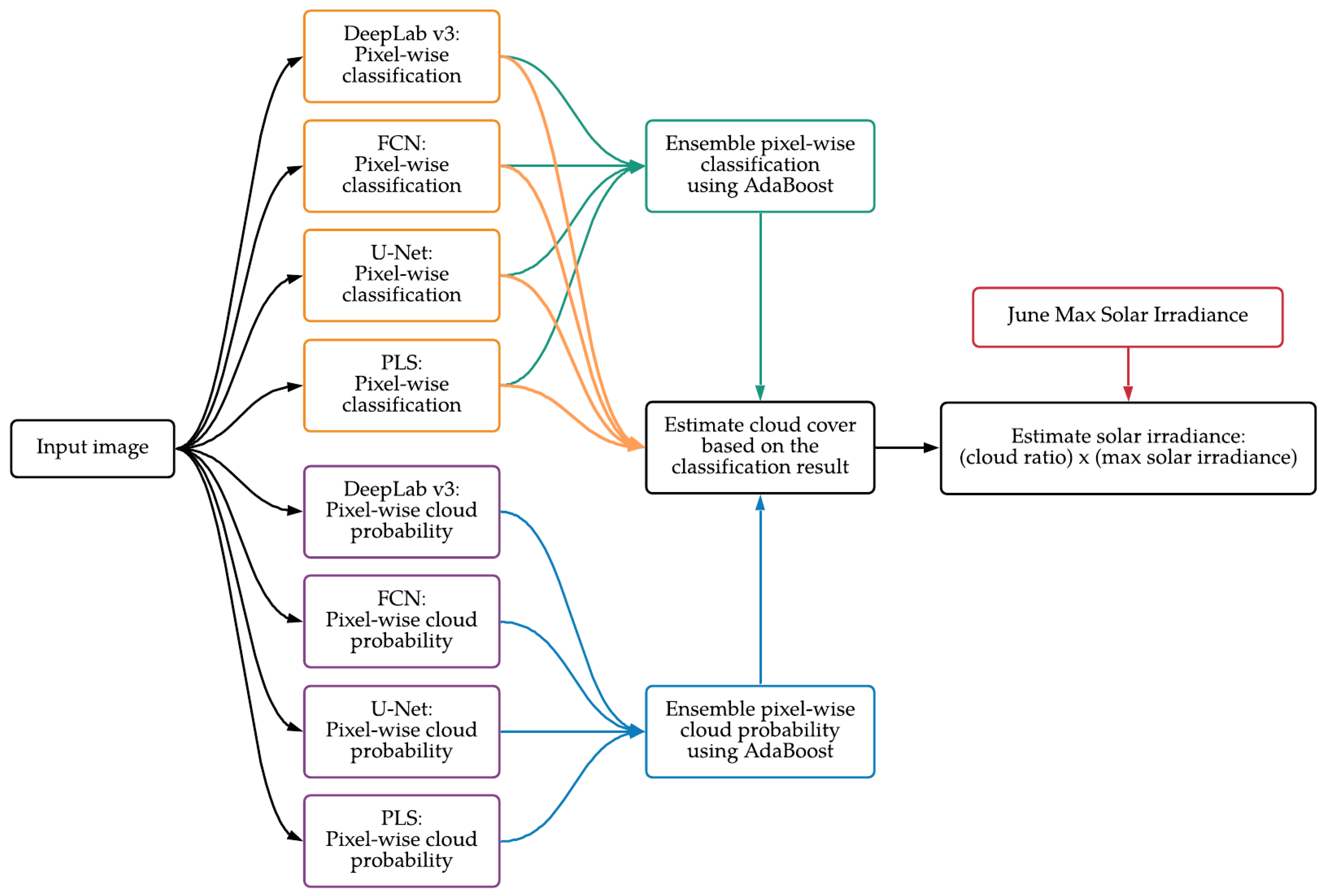
2.3. Ensemble Method

The AdaBoost machine learning method is one of the first boosting algorithms. We adopted it to integrate the outputs of different machine learning algorithms (weak learners, in boosting algorithms parlance) into a weighted strong model to improve the accuracy of the final output. The weak learners are decision trees in AdaBoost. The method recognizes outliers and noise from the output of weak learners and adjusts weights on weak learners based on the detected outliers and noise to reduce misclassified instances. AdaBoost is less susceptible to overfitting than other boosting algorithms [35] are. As the tree grows deeper, the algorithm focuses more on cases that are difficult to classify or regress. We trained two AdaBoost models: the first a regression model with the outputs of cloud probability of each pixel from the machine learning methods and the second with the classified class number of each pixel. The maximum depth of the models was 4, and the number of estimators was 200 for each model. Details on how we trained the models are introduced in Section 4. As with the PLS regression model, both AdaBoost models were tested with different threshold values to find the most suitable value. The selected thresholds were 0.7 for the AdaBoost model trained with class numbers and 0.6 for the AdaBoost model trained with normalized cloud probability.

3. Datasets

To train machine learning models for cloud coverage estimation, we utilized three cloud image datasets: SWIMSEG [18,19], HYTA [17], and the Waggle cloud dataset that we created for this research. Next, we briefly describe these three datasets.

3.1. Singapore Whole Sky Imaging Segmentation Database

The SWIMSEG database was created by the Advanced Digital Science Center at the University of Illinois at Urbana-Champaign and the Nanyang Technological University, Singapore for color-based cloud segmentation to find suitable color components among various combinations of color channels to separate cloud and sky pixels [18,19]. It contains 1013 images of the sky and corresponding manually labeled binary ground truth. The binary images represent sections of the sky and cloud colored in black and white pixels, respectively. Scenes in the dataset were produced by a camera using a fisheye lens with 180 field of view, followed by postcapture processing taking into account the angle of azimuth and elevation and other camera parameters in order to correct distortion. The boundaries of clouds are clearly distinguishable in the images based on color.

3.2. Hybrid Thresholding Algorithm Database

The HYTA database is another publicly accessible cloud image dataset [17] consisting of 32 pairs of sky images and manually labeled binary annotations created from whole-sky cameras located in Beijing and Conghua in China. Unlike the SWIMSEG dataset, the HYTA images are not postcapture processed to correct distortion. The dataset also contains additional images from alternate viewpoints (non-upward-facing camera) to increase the diversity of the dataset. The majority of the images in HYTA show clear boundaries between clouds and sky, with distinguishable colors, well suited for their research goal of using diverse thresholds for different color components to separate cloud pixels from sky pixels.

3.3. Waggle Cloud Dataset

The two datasets SWIMSEG and HYTA provide images that show clear boundaries between the sky and clouds. To supplement these with images having thin clouds and overcast conditions, we created a new dataset using the Waggle platform [36]. Waggle is an extensible internet-connected and field-deployable edge computing platform for wireless sensing and running artificial intelligence and machine learning (AI/ML) algorithms. A variety of sensors including cameras, environmental sensors, microphones, and LiDARs can be integrated into the nodes, which support in situ computation and AI/ML through single-board computers with AI/ML accelerators.
We deployed a Waggle node with a sky-facing camera with a field of view of 67 , capable of capturing images with dimensions of 2304 × 1536 pixels. A single-layer plastic dome provided environmental protection to the camera. The images were collected in Lemont, IL, USA, every 15 s and transferred to a central image repository without any preprocessing. The reflection and diffraction of sunlight captured in the images of the dataset due to the protective dome or other physical elements were not filtered out. The images from both “bright and sunny” and overcast days were curated for this dataset, manually excluding views that were saturated by bright sunlight. (Automated methods to isolate images overpowered by sunlight will be explored in the future.) The images in the Waggle cloud dataset were manually labeled as shown in Figure 2 using OpenCV through a two-step process. First, pixels were labeled based on saturation, red, and blue values. By adjusting the threshold of the three color channels, the cloud and sky pixels were roughly separated. Second, pixels that were difficult to separate through the threshold adjustment were manually labeled.

3.4. Solar Irradiance and Solar Power Product Measure
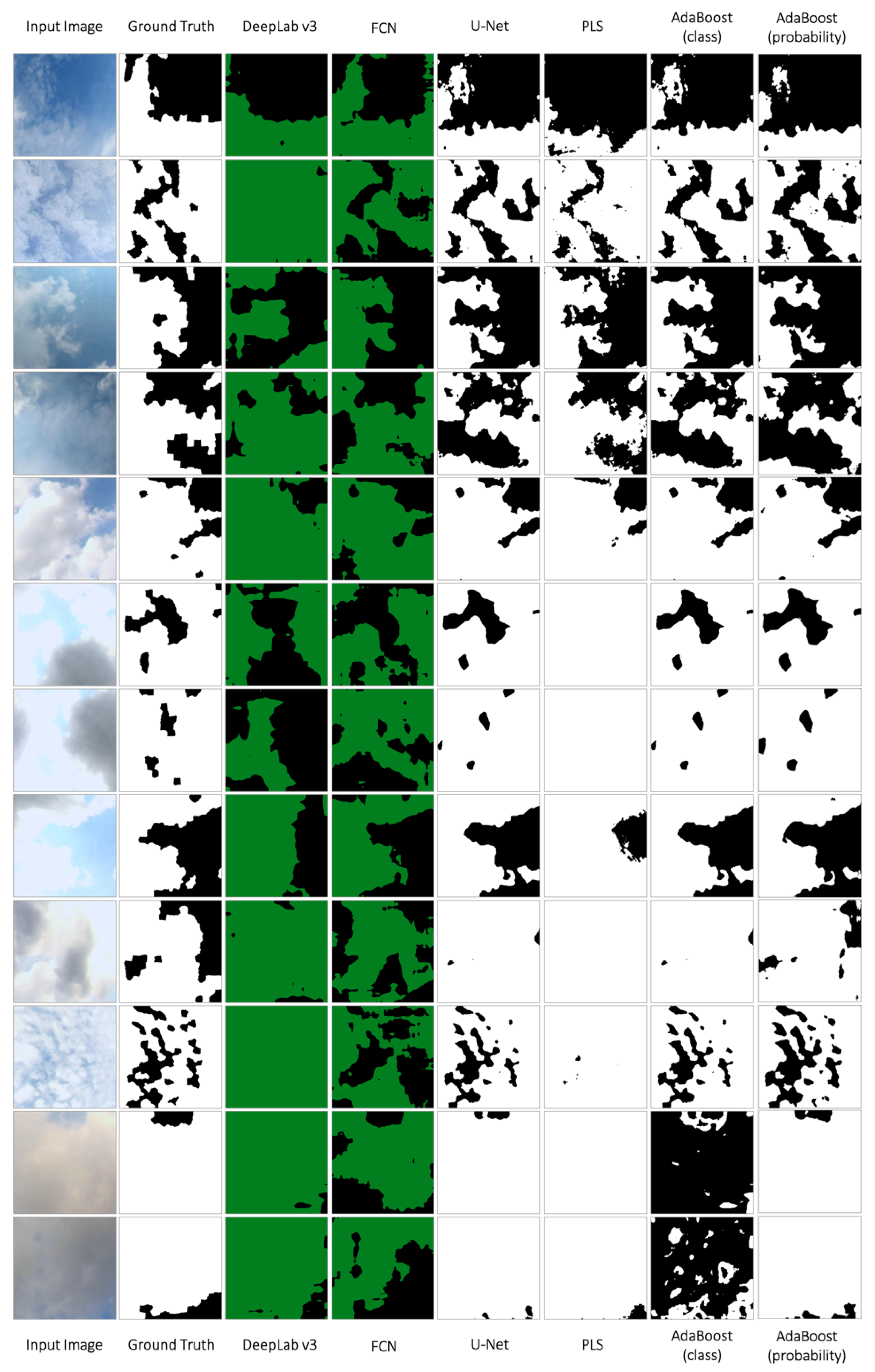
To analyze the relationships between solar irradiance, solar power production, and cloud cover, we utilized measurements of net solar irradiation and global irradiation from the Argonne National Laboratory meteorological sensor tower. The tower website provides current and historical meteorological data [37]. Total solar power product was obtained from the photovoltaic array deployed at the Argonne Energy Plaza. Real-time and historical solar power product and power usage data are available at [38]. The meteorological sensor tower and photovoltaic array have a clear and unobstructed view of the sky, with the meteorological sensor tower about 100 m southwest of the Waggle node and the photovoltaic array about 1600 m northeast of the node. The published solar irradiance values are averages over 15 min, and power production is published as an instantaneous measurement every 5 s.

4. Model Validation

The models trained with the Waggle and SWIMSEG datasets were tested for their efficacy on cloud pixel segmentation. We used 160 images from the SWIMSEG dataset (excluding the images used for training and validation) and 32 images from the HYTA dataset to validate the models. Sampled cloud segmentation results are shown in Figure 3. In the figure, the first column is the raw sky image, and the second column is the “ground truth” labeled manually. The rest of the columns show the results, respectively, from FCN, U-Net, color-based segmentation using PLS regression, DeepLab v3, AdaBoost regression trained with class numbers, and AdaBoost regression trained with normalized cloud probability. Pixels segmented as white or green in the figure are cloud pixels, and black pixels are sky pixels.
The top five images in Figure 3 show relatively clear boundaries between the clouds and sky; the blue features are clearly visible in the sky pixels. In comparison, the separation is weaker in the next five images, and the last two images show overcast conditions. When the sky is partially cloudy and the blue features are clearly visible (top five images), the majority of the models are able to segment cloud pixels reasonably well, with the DeepLab v3 model overestimating cloud pixels in comparison with other models. In this case, the machine learning models seem to perform better than humans at segmenting cloud pixels, as seen in the ground truth images. This is evident in the second and third rows in Figure 3. One can see that while humans segment coarsely, the models are more fine-grained. In the next five images where blue features in sky pixels are relatively weaker, the PLS model overestimates cloud pixels, and the FCN and DeepLab v3 models underestimate them.
From the results (rows 6–12 in Figure 3), we note that U-Net overestimates cloud pixels in overcast conditions or when there are multiple layers of clouds and the colors of the cloud layers are significantly different. Additionally, when there are multiple layers of clouds with large variability in cloud thickness across the image, the different cloud layers are significantly distinguishable, and the DeepLab v3 model classifies dark pixels as sky and bright pixels as clouds. Because of the misclassification, the lower dark cloud pixels are segmented as sky pixels, and the bright cloud and sky pixels are segmented as sky for the samples shown in Figure 3 (the 6th and 7th rows). The FCN model has trouble finding boundaries between dark and bright pixels; therefore, some of dark cloud pixels are segmented as sky, and some of the bright sky pixels are segmented as cloud pixels in the sampled results in Figure 3, row 7. When the sky is mostly overcast, the FCN model has the same difficulty in determining boundaries between cloud and sky, and AdaBoost trained with class-number-segmented cloud and sky pixels inversely, as shown in the last two rows in the figure.
The segmentation accuracy of each model for the test images is shown in Table 1. U-Net is the most accurate model for all three measures: mean intersection over union (mIoU), mean average precision (mAP), and mean average recall (mAR) for the test images. The second-best model for cloud segmentation is DeepLab v3 in terms of mAP, and PLS is the second best for mIoU and mAR. In this research, the models have only two classes, cloud and sky, because the binary classification is coherent in terms of identifying cloud pixels. Therefore, all types of clouds that are thin or thick are segmented as the same class: cloud.

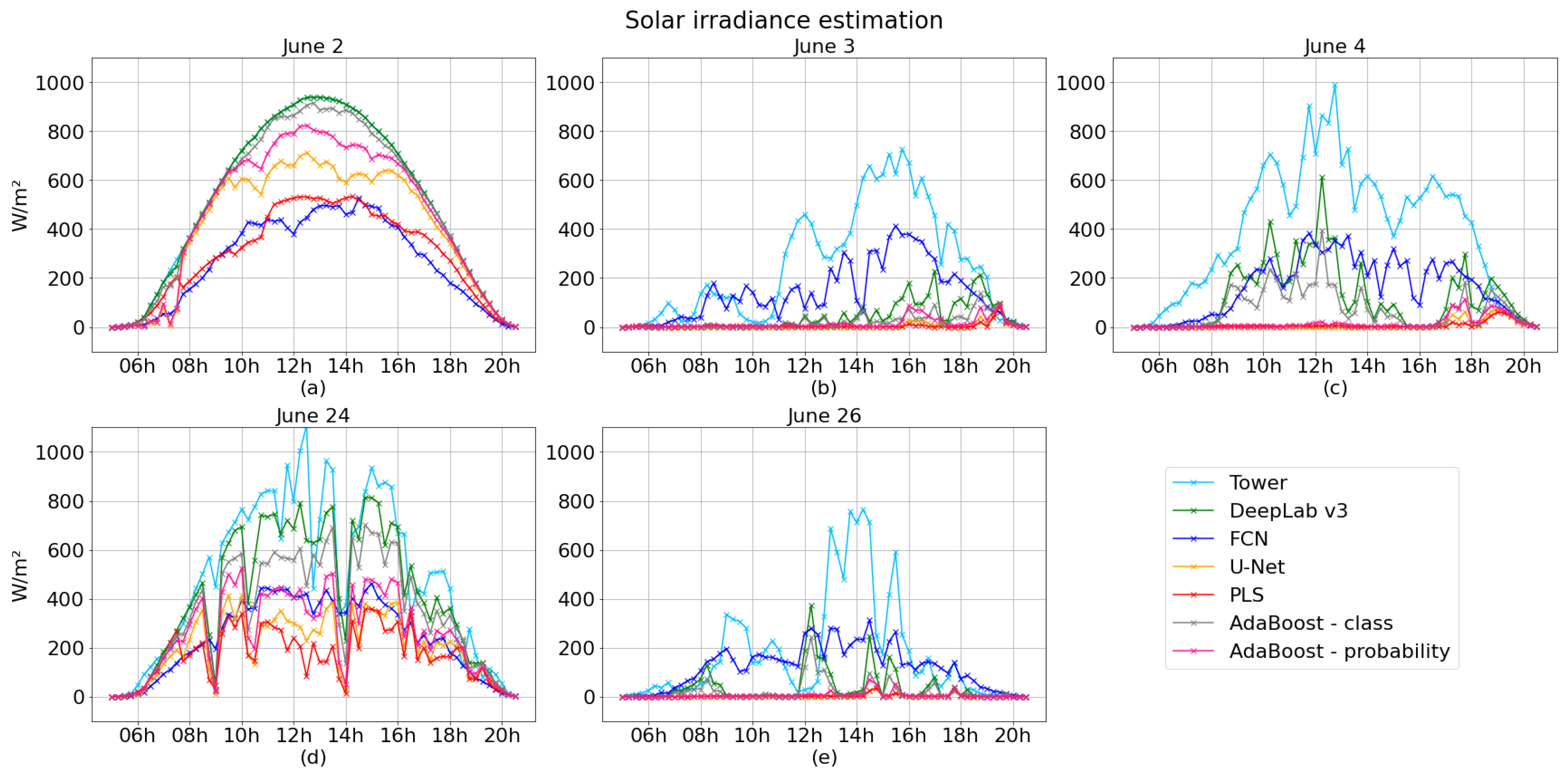
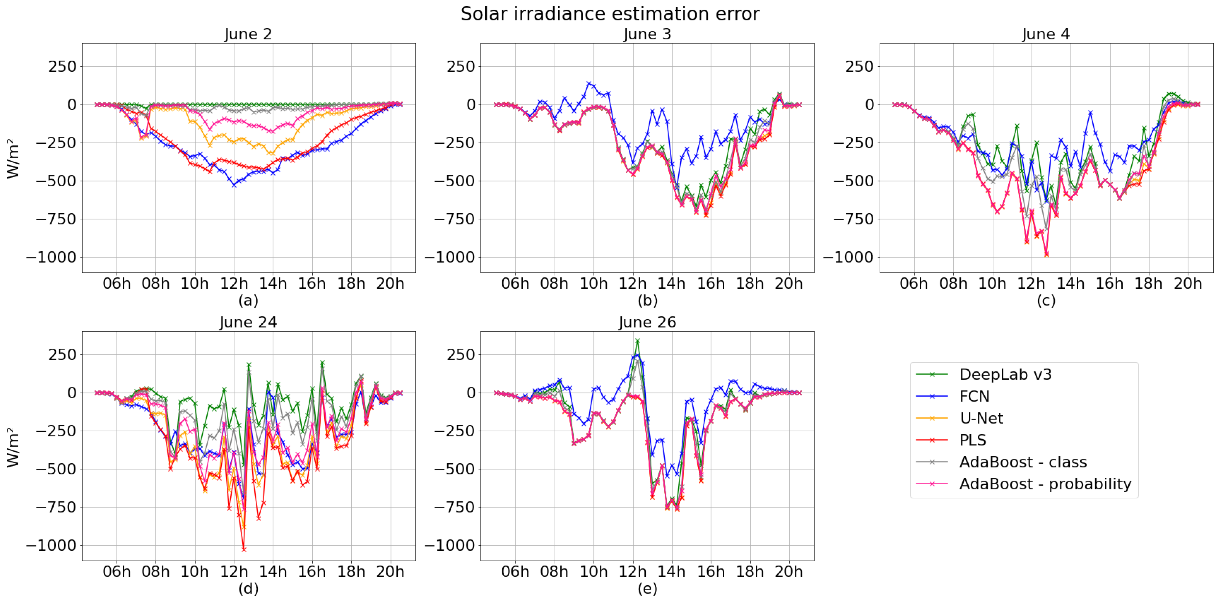
5. Solar Irradiance Estimation

With the validated models, we estimated solar irradiance using data collected from Argonne’s meteorological sensor tower, Argonne’s Energy Plaza, and the Waggle node. We chose data from 14 days in June 2020, continuously collected in the daytime from these sources. From these data, the change in the cloud cover ratio and the solar irradiance can be tracked synchronously throughout each day. Solar irradiance values were estimated by using the cloud cover ratio from the cloud segmentation models.

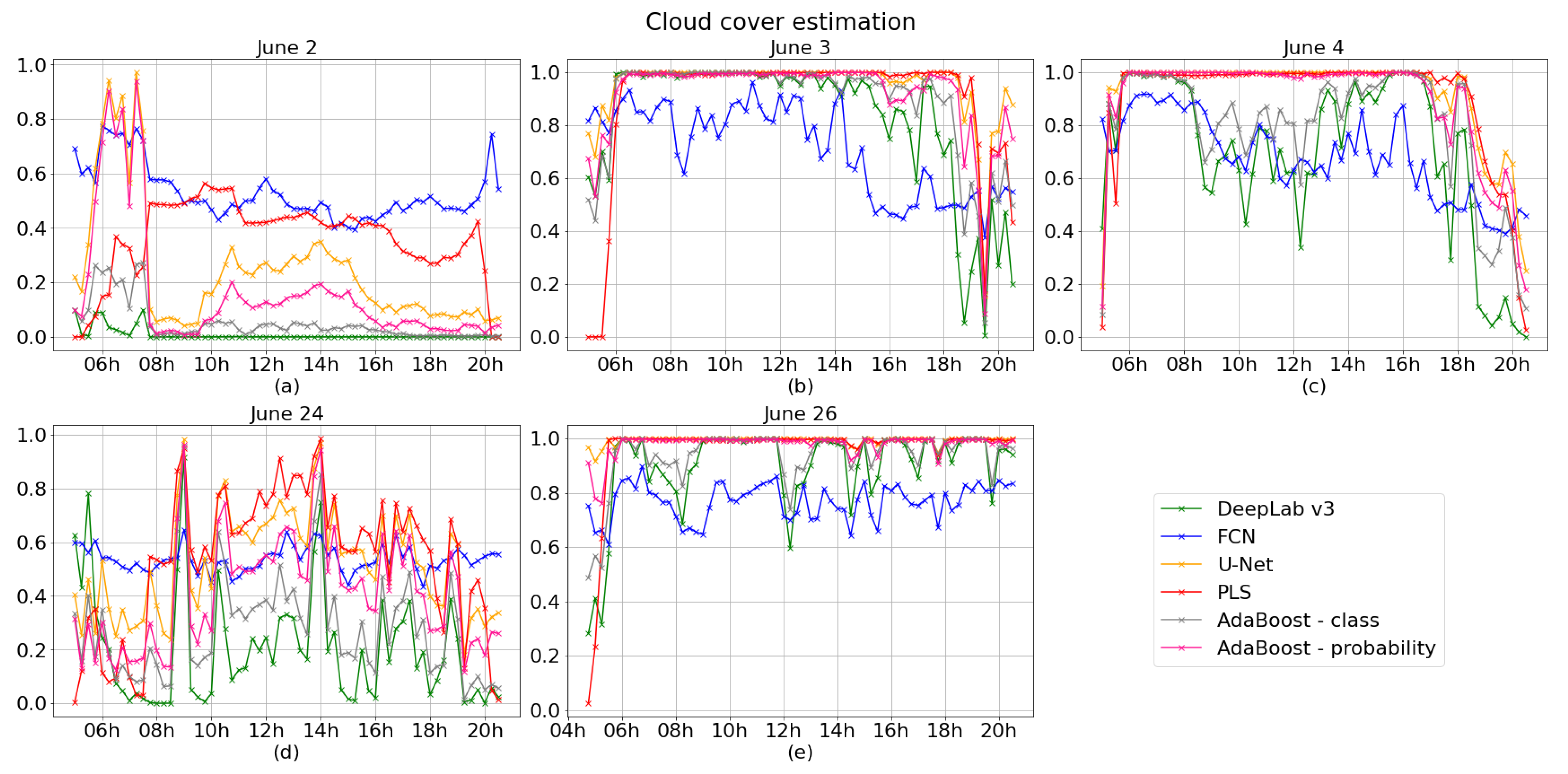
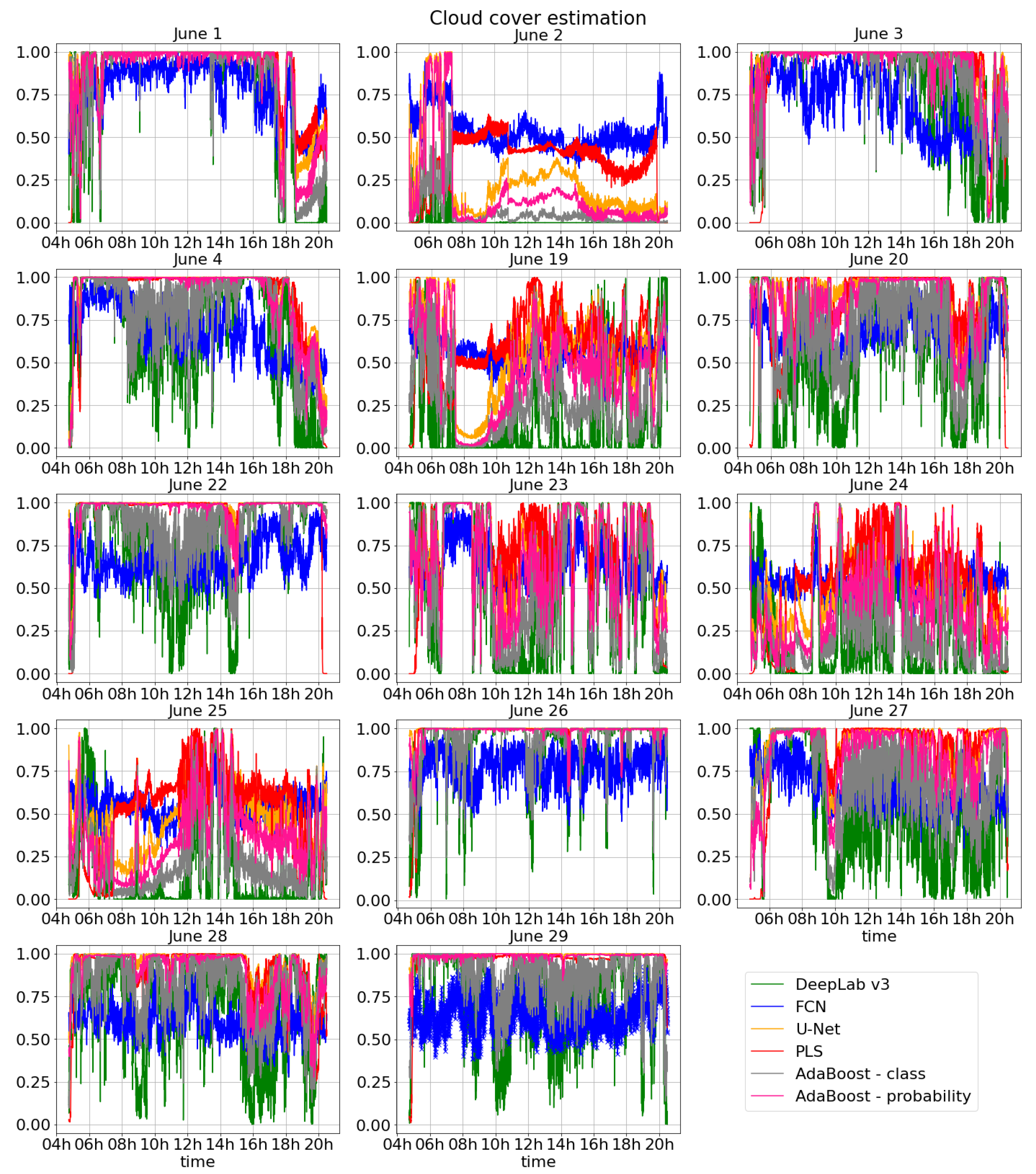
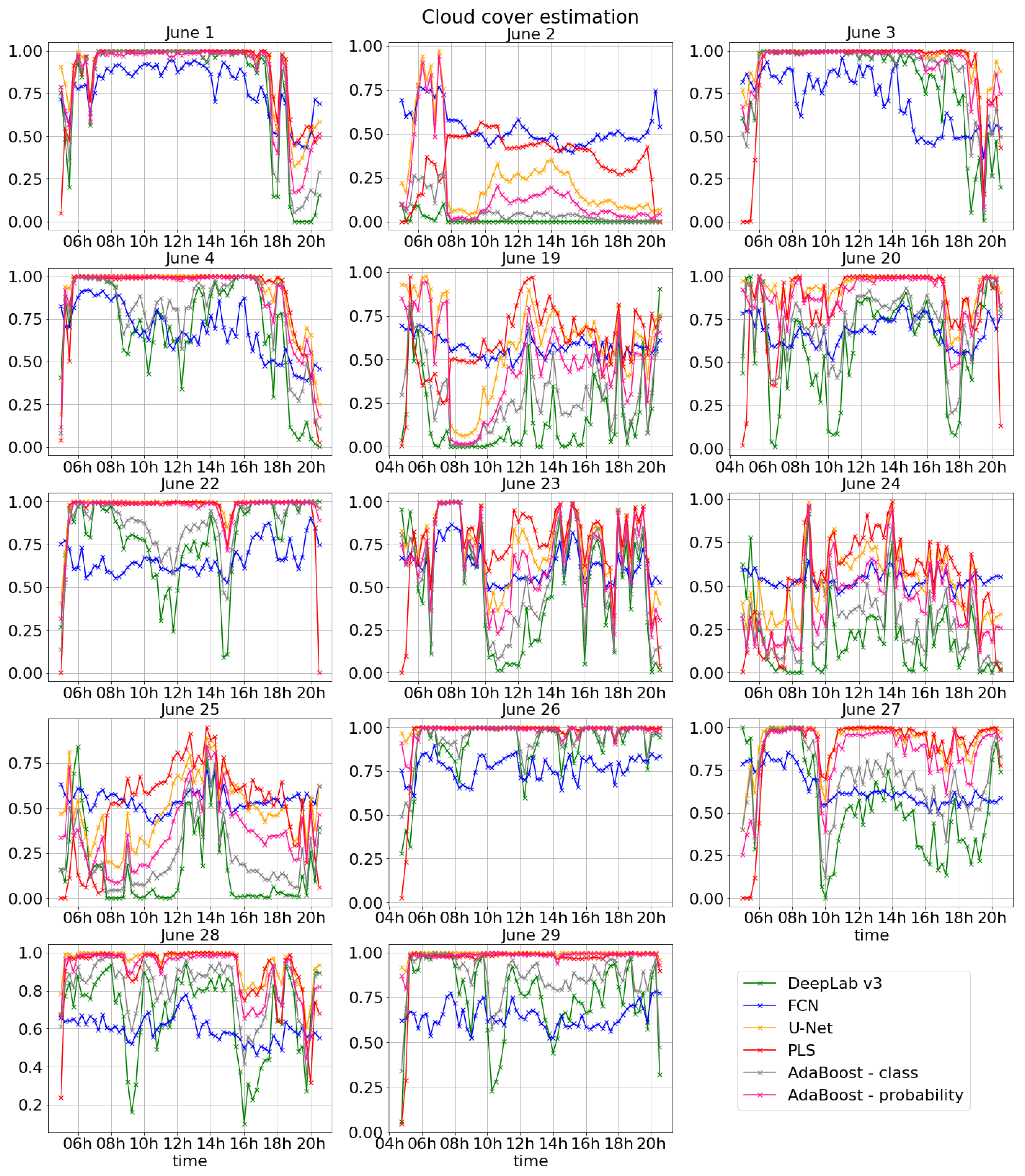
5.1. Cloud Cover Estimation

The Waggle node collected sky images every 15 s from 4:45 a.m. to 10 p.m., resulting in a total of 64,649 images collected during our 14-day window in June. From the images, we selected images collected from approximately 10 min prior to sunrise to 30 min after sunset (5 a.m. to 9 p.m.). Thus, 50,983 images were selected and used to estimate cloud cover. Because of the occasional instability of the network where the Waggle node was deployed, the selected number of images per day is not constant, as shown in Table 2.
The cloud cover ratio using the machine learning models was estimated with the selected images. Each model segments cloud pixels as described in Section 2. The FCN and DeepLab v3 models choose a higher probability class, either cloud or sky; the U-Net model utilizes a sigmoid function; and regression models use thresholds to determine whether each pixel is cloud or sky. Figure A1 shows the cloud cover estimation results for the 14 days using the images collected every 15 s. The estimation results were averaged for every 15 min as shown in Figure A2 to match with the time interval of the measured solar irradiance from the Argonne meteorological sensor tower. The figure shows the ratios of cloud pixels in the images. If no cloud pixel was detected, the ratio was calculated as 0; and if the whole sky was covered with cloud, the ratio was calculated as 1.
We selected five days from the 14 days that cover the different cloud conditions: clear sky, partially cloudy sky, haze clouds, and overcast clouds. In Figure 4, Figure 4a is the clear sky, Figure 4b,c are haze clouds, Figure 4d is partially cloudy sky, and Figure 4e is overcast clouds. Detailed cloud pixel classification results can be found from the images at the bottom of Appendix A.2.1, Appendix A.2.2, Appendix A.2.3, Appendix A.2.4, Appendix A.2.5. We found that the U-Net deep learning model was especially sensitive to the identification of thin and brightly colored cloud pixels when compared to the other models (Figure 4d). This model reported a higher cloud cover ratio when the sky was partially cloudy and a thin cloud layer covered the sky, as shown in the figure. The PLS model reported the highest cloud cover because the model did not segment well when the saturation values were high in both cloud and sky pixels as shown in Figure 4a. The PLS model identified only sky pixels that had distinguishable blue features. In contrast to the U-Net, the DeepLab v3 algorithm performed poorly when the sky contained thin cloudlets as shown in Figure 4d. Because the DeepLab model was developed to understand and segment objects in a context, it appears that DeepLab understood “cloud” and “sky” only as large regions of the image. When the bright and dark cloud layers were combined in the scene, both DeepLab v3 and FCN models did not work well; when the sky was covered with cloudlets with a variety of thickness, the models failed to separately recognize the layers as shown in Figure 4b–e. On a partially cloudy day, the FCN model also failed to recognize the difference between bright cloud pixels and bright pixels caused by reflection of sunlight similar to PLS model, as shown in Figure 4d and Figure A6. The performance of the models we used to estimate cloud cover varied significantly (Figure A2). The details of model-specific cloud recognition results and solar irradiance estimation in different sky types are discussed in Section 5.2.

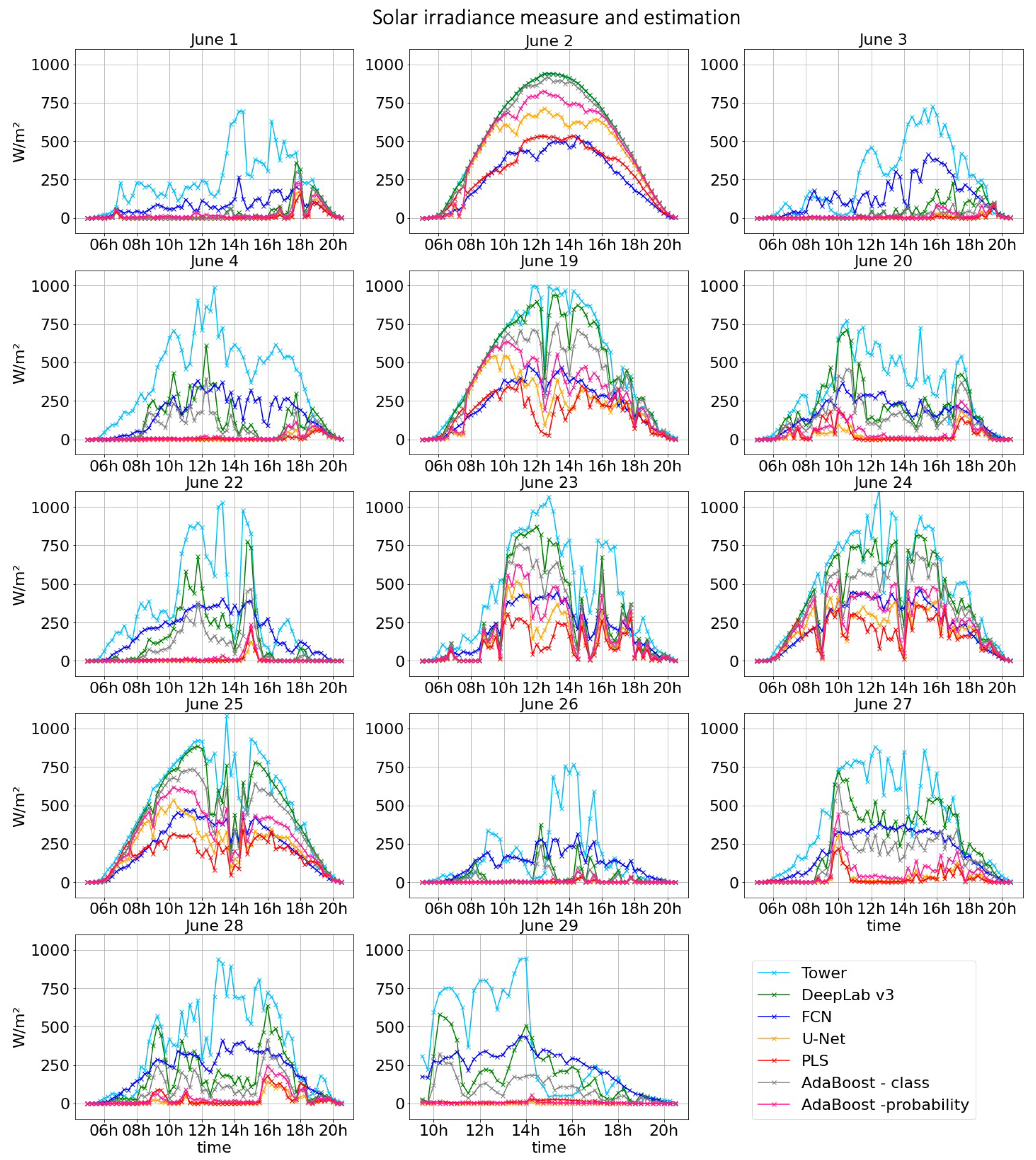
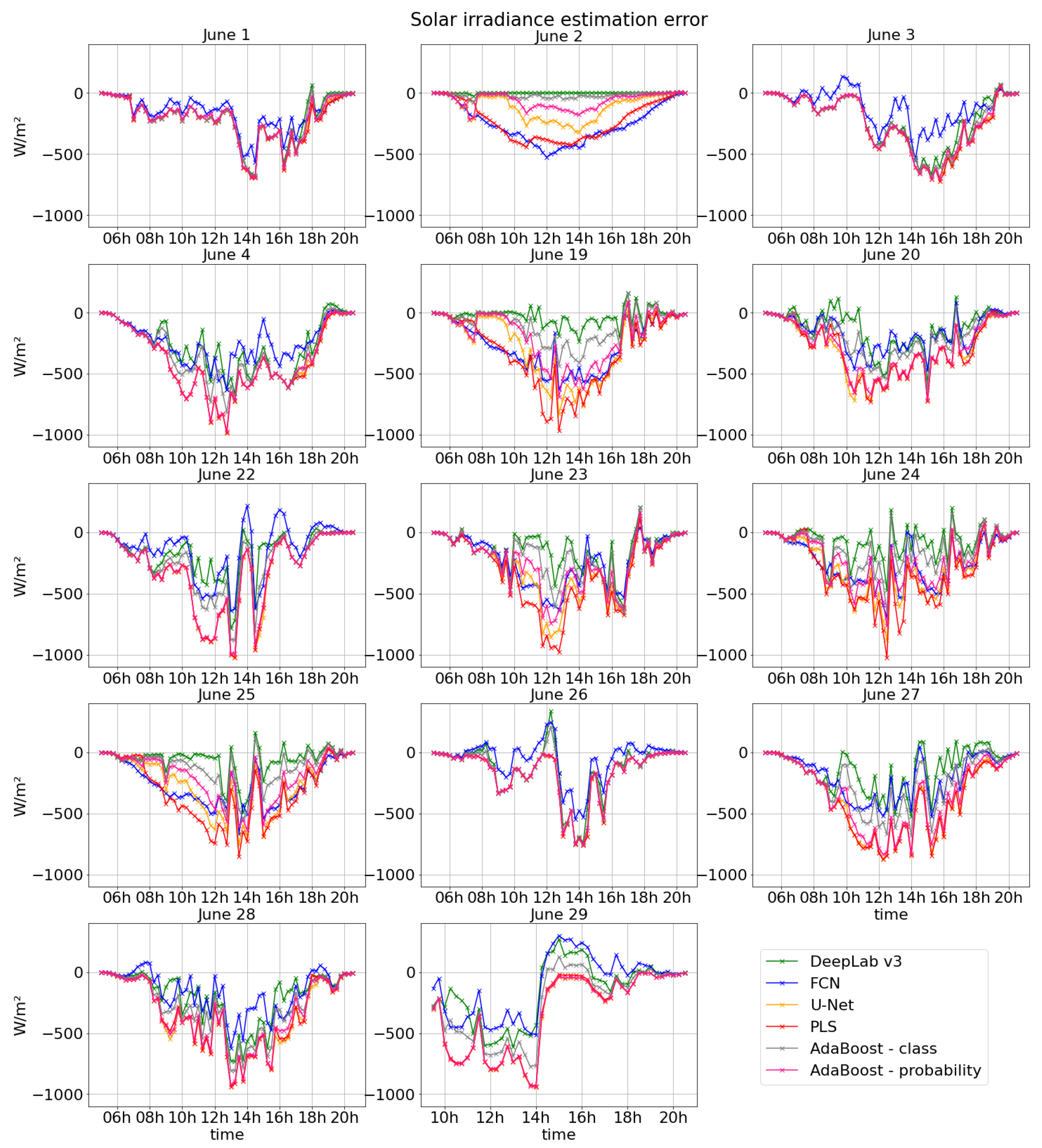
5.2. Solar Irradiance Estimation

Various approaches for parameterizing and modeling the relationship between cloud and solar irradiance have been studied. Martins et al. [39] estimated solar irradiance using the cloud cover index (CCI). They described solar irradiance as a linear combination of clear and overcast day CCI. Lengfeld et al. [40] parameterized and created a solar irradiance model using features from clouds and the sun. Moreover, in a recent study, Badescu and Dumitrescu [41] modeled the relationship between cloud and solar irradiance nonlinearly to solve the inconsistency of models according to sky condition.
We estimated solar irradiance using the maximum solar irradiance measurement and the cloud cover inference results as described in Section 2. Based on the maximum solar irradiance and cloud cover estimation results, the solar irradiance of the 14 days was predicted, as shown in Figure A3. We selected five representative days for (a) clear sky, (b,c) haze clouds, (d) partially cloudy sky, and (e) overcast clouds as shown in Figure 5. The light blue lines in the figure are the measures from the Argonne meteorological sensor tower that are the ground truth of solar irradiance.
The five selected days represent four cases for detailed analysis: clear, haze cloudy, partially cloudy, and overcast with mixture of thin and thick clouds. The results for these four situations are as follows:
Clear sky: Figure 5a and Figure A5 show solar irradiance estimation of a clear day, the error of estimation in W/m 2 , and cloud cover segmentation results from the models. Most of the models segmented bright pixels that occurred because of the sun and reflection of sunlight as cloud pixels because no preprocessing was performed on the input images and the images were collected from a device without equipment shading the sun. The DeepLab v3 model and AdaBoost model trained with class numbers had less confusion between cloud pixels and sunlight, resulting in smaller errors of solar irradiance estimation compared with those of the other models.
Cloudy sky: Figure 5d and Figure A6 show solar irradiance estimation of a partially cloudy day, the error of estimation in W/m 2 , and cloud cover segmentation results from the models. The cloud pixels segmentation results in the figure indicate that the AdaBoost model trained with class numbers was able to separate cloud pixels more accurately than were the other models. The model was able to separately distinguish dark cloud and sky pixels, and it also was able to segment tiny cloud pieces that were floating around a large piece of clouds, which are difficult to segment manually. The DeepLab v3 model also was less sensitive to the small floating slice of clouds. Both models identified separated small pieces of clouds as one large chunk with the main large cloud. Among the models, AdaBoost trained with class numbers and the DeepLab v3 model were able to distinguish bright sky pixels and cloud pixels more precisely so that the solar irradiance errors were relatively smaller than the errors from other models, as well as in the clear day case.
The last two cases are haze clouds and overcast with mixture of thin and thick clouds. The results for haze clouds are shown in Figure 5b,c, and the results for overcast with mixture of thin and thick clouds are shown in Figure 5d. Solar irradiance estimation, the error of estimation in W/m 2 , and cloud cover segmentation results from the models are shown in Figure A7 and Figure A8 for haze clouds and Figure A9 for overcast clouds. Figure A7 and Figure A8 show that the AdaBoost model trained with class-number-segmented cloud pixels that were the inverse of the results from FCN. Because the AdaBoost models is an ensemble of segmentation results from four machine learning models, we can hypothesize that the model concluded that the class classification results from FCN were the inverse of the ground truth with high probability when thin clouds cover the sky. For both haze and overcast cases, the AdaBoost model trained with cloud probability and the U-Net model segmented cloud pixels most accurately, as the figures show. The models understood features of both thin and thick clouds and were able to classify the pixels as clouds. However, the accuracy of the cloud pixel segmentation was not directly related to the accuracy of solar irradiance estimation in these cases because the proposed method did not separately weigh sunlight penetration with regard to cloud thickness. The proposed method assumed that all types of cloud pixels blocked sunlight even if the cloud layers were thin. Therefore, the solar irradiance was under-estimated. From the results of the two cases, we recognize that in order to improve the performance of the solar irradiance estimation, one must separately detect and segment different cloud types and thicknesses.
Overall, the DeepLab v3 model estimated solar irradiance most accurately, and the standard deviation of errors of FCN was the smallest. The solar irradiance estimation errors in the 14 days are shown in Figure A4, and the representative five days are shown in Figure 6. When the day was clear and sunny, the error significantly decreased in most models, as shown in Table 3 and Figure 6a. Most important, when the sky is partially cloudy, the solar irradiance value can vary rapidly and affect solar panel performance. As shown in Figure 6d, the DeepLab v3 model estimates the solar irradiance with approximately 66% accuracy. When the model adopts a method for cloud thickness separation, we expect that the accuracy will increase.

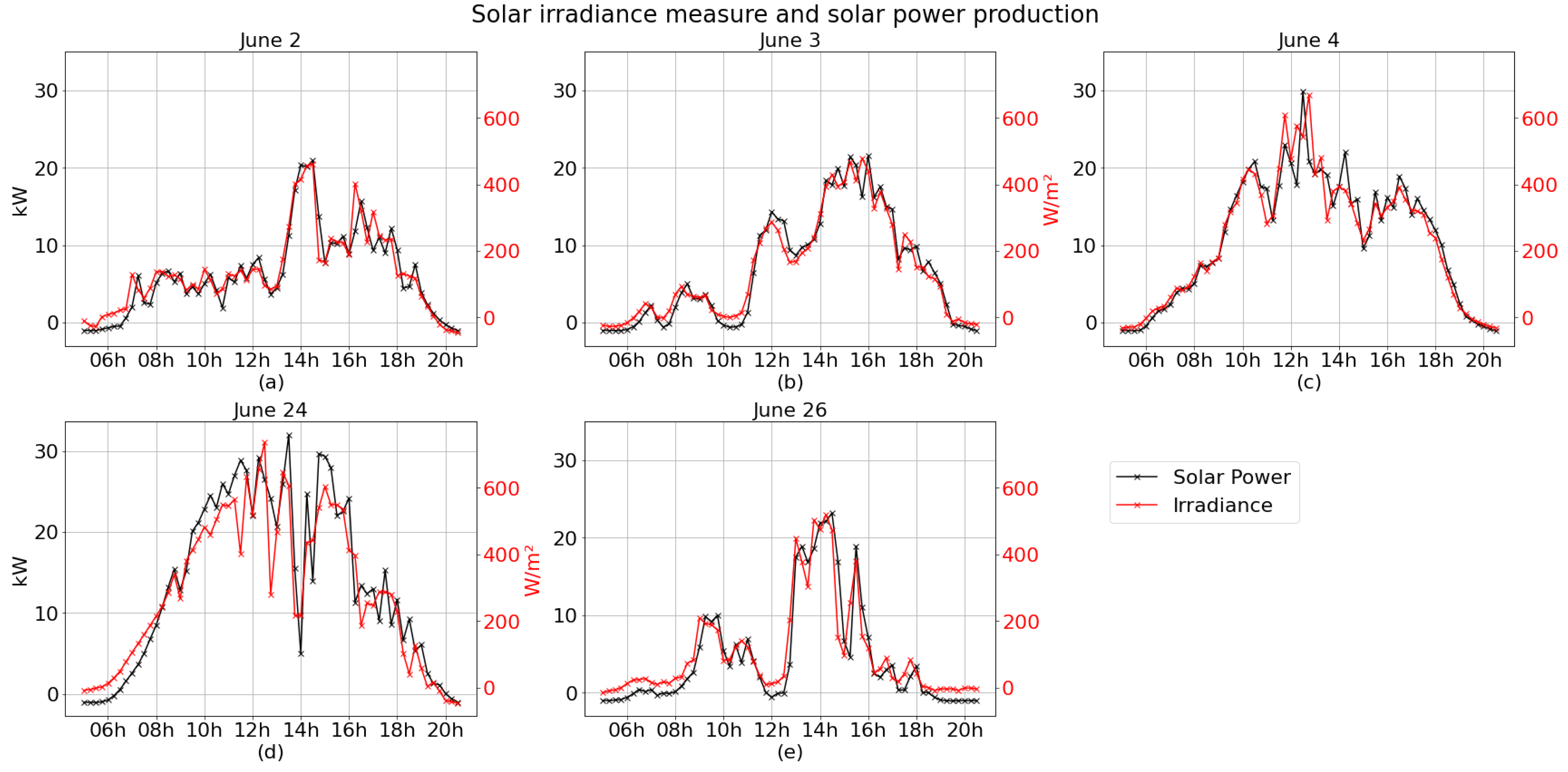
5.3. Solar Power Product Estimation

Solar irradiance is highly correlated with solar power production from photovoltaic panels. Figure A10 shows the measured solar irradiance from Argonne’s meteorological sensor tower and solar power production from Argonne’s Energy Plaza during the 14 days used for this work, and the representative five days are shown in Figure 7. Figure 8 and Figure A11 show the difference between solar irradiance measure and solar power production in the 5 days. As the figures show, the two measures are highly correlated in all days under multiple types of clouds. Because the Energy Plaza, where the photovoltaic arrays are placed, is located approximately 1380 m southeast of the meteorological sensor tower, the two measures show variations. The variations occurred according to changes in sky conditions, such as direction and speed of cloud movement. When the sky condition was constant, such as clear or hazy all day (for example, on 1–3 June 2020), the variations were smaller than on a partial cloudy day (28 June 2020). However, the two measures show similar trends, decreasing and increasing their value over the same period of time. Therefore, we can conclude that estimation and forecasting of solar irradiance based on cloud cover can be projected to solar power production.

6. Conclusions and Future Work

In this paper, we proposed a method to predict solar power production by estimating solar irradiance from sky-facing cameras by using machine learning techniques to compute cloud cover ratio. We trained and validated six machine learning models to measure cloud cover: DeepLab v3, FCN, U-Net, PLS regression, and two AdaBoost models. The AdaBoost models were trained with two different types of results obtained from the other four machine learning models in a conservative manner: one type was classification results if each pixel was sky or cloud, and the other was probability of how much each pixel could be classified as cloud. The software used in this study is available in the Waggle repository (https://github.com/waggle-sensor/solar-irradiance-estimation, accessed on 11 February 2021). The cloud cover estimation results presented in Section 4 show that the deep neural networks performed appropriately for segmentation of cloud pixels. The results demonstrate that the performances of each model for cloud segmentation were different because each machine learning model had its own attributes to recognize and identify features from input images. Among the models, U-Net was the most accurate model for cloud pixel segmentation.
We estimated solar irradiance using the measured cloud cover and maximum solar irradiance, as shown in Section 5.2. Solar irradiance estimation was most accurate using the DeepLab v3 model. We observed that cloud cover was correlated with solar irradiance and that solar irradiance was highly correlated with solar power production. Thus solar power production can be estimated from cloud cover.
We observed that inconsistencies between cloud cover measure and solar irradiance estimation occurred because the method classifies only cloud vs. sky. By grouping various types and thicknesses of cloud pixels into the same category, the method could not support a sunlight penetration level that might be determined by cloud features (such as thickness). Underestimating solar irradiance on hazy and overcast days can be resolved by improving the cloud segmentation to classify cloud pixels with regard to thickness and type.
Developing methods to distinguish cloud thickness or type can be challenging, however. This augmented segmentation will require annotated images with known cloud thickness. The extra data may be obtained from infrared camera images that provide thermal information of clouds or other meteorological sensor data that can help estimate cloud thickness or sunlight transmittance through the cloud. We expect that an improved cloud cover measure method can be utilized to improve our estimation of solar irradiance. Other improvements may be achieved by using video to incorporate cloud motion (speed and direction) and cloud formation/dissipation. By deploying the machine learning prediction application on an edge computing platform, such as Waggle [36] or SAGE [42], it will be possible to provide real-time, in situ estimates of solar irradiance and solar power production.

Author Contributions

Conceptualization, S.P., Y.K., N.J.F., S.M.C., R.S. and P.H.B.; methodology, S.P., Y.K., N.J.F., S.M.C. and R.S.; software, S.P. and Y.K.; validation, S.P., Y.K., N.J.F., S.M.C. and R.S.; formal analysis, S.P., Y.K., N.J.F., S.M.C. and R.S.; investigation, S.P., Y.K. and R.S.; resources, R.S. and P.H.B.; data curation, S.P., Y.K., N.J.F. and R.S.; writing—original draft preparation, S.P.; writing—review and editing, S.P., Y.K., N.J.F., S.M.C., R.S. and P.H.B.; visualization, S.P.; supervision, S.M.C., N.J.F.; project administration, P.H.B.; funding acquisition, P.H.B. All authors have read and agreed to the published version of the manuscript.

Funding

The Waggle platform design was supported through Argonne National Laboratory’s Laboratory-Directed Research and Development program, LDRD: 2014-160-N0. The SAGE project is funded through the U.S. National Science Foundation’s Mid-Scale Research Infrastructure program, NSF-OAC-1935984 [42]. This material is based upon work supported in part by U.S. Department of Energy, Office of Science, under contract DE-AC02-06CHI1357, and analysis work was supported by Exelon Corporation through CRADA T03-PH01-PT1397.

Institutional Review Board Statement

Not applicable.

Informed Consent Statement

Not applicable.

Data Availability Statement

The Waggle cloud dataset is available from the authors after agreeing to the data usage policy of Waggle.

Acknowledgments

We thank Theresa M. Christian and Uuganbayar Otgonbaatar at Exelon for valuable discussions and feedback. Additionally, We thank Sean Shahkarami and Emil M. Constantinescu at Argonne National Laboratory for discussions, feedback, insights, and ideas for this work. Moreover, we thank Goeum Cha at Purdue University for assisting in implementing the color-based cloud segmentation method. We also thank Gail W. Pieper at Argonne National Laboratory for constructive criticism of the manuscript.

Conflicts of Interest

The author declares no conflict of interest.

Appendix A. Results

Appendix A.1. Cloud Cover Estimation Results

Figure A1. Cloud cover estimation results for the 14 days.
Atmosphere 12 00395 g0a1
Figure A2. Results of 15 min-averaged cloud cover estimation for 14 days. The results show ratios of cloud pixels in images at each time point. If no cloud pixel was detected, the ratio was calculated as 0; if the whole sky was covered with cloud, the ratio was calculated as 1.
Atmosphere 12 00395 g0a2

Appendix A.2. Solar Irradiance Estimation Results

Figure A3. Measured solar irradiance (light blue) and solar irradiance estimation results in W/m 2 using 15 min-averaged cloud cover estimation and maximum solar irradiance measured on 2 June 2020 for 14 days. The tower measure on 2 June ( b l u e l i n e ) is overlapped with the DeepLab v3 estimation results ( g r e e n l i n e ), with only a small observable difference between these at 7–8 h.
Atmosphere 12 00395 g0a3
Figure A4. Solar irradiance estimation error in W/m 2 for 14 days.
Atmosphere 12 00395 g0a4

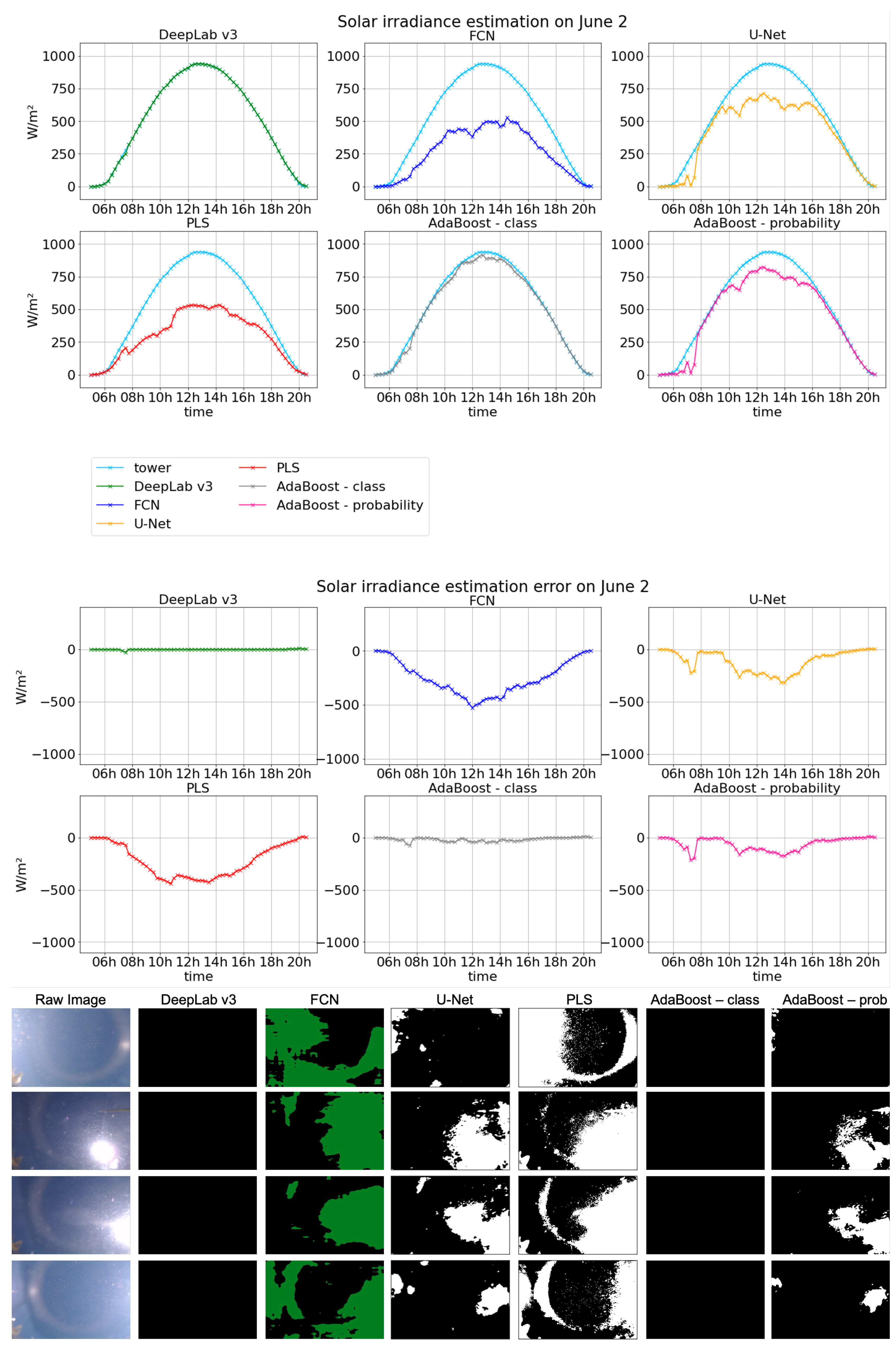
Appendix A.2.1. 2 June 2020

Figure A5. Solar irradiance estimation results based on cloud cover estimation from each machine learning model on 2 June 2020.
Atmosphere 12 00395 g0a5

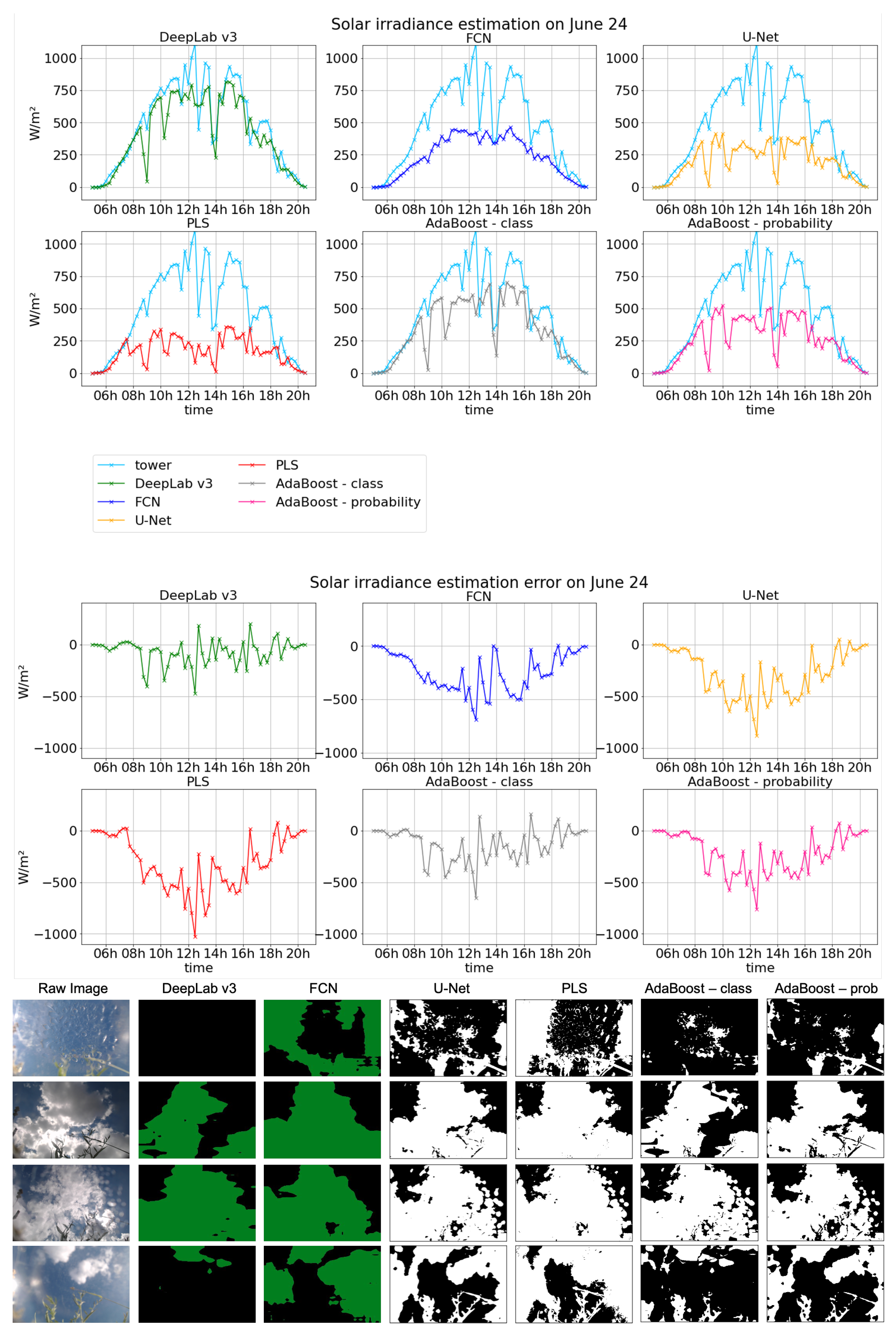
Appendix A.2.2. 24 June 2020

Figure A6. Solar irradiance estimation result based on cloud cover estimation from each machine learning model on 24 June 2020.
Atmosphere 12 00395 g0a6

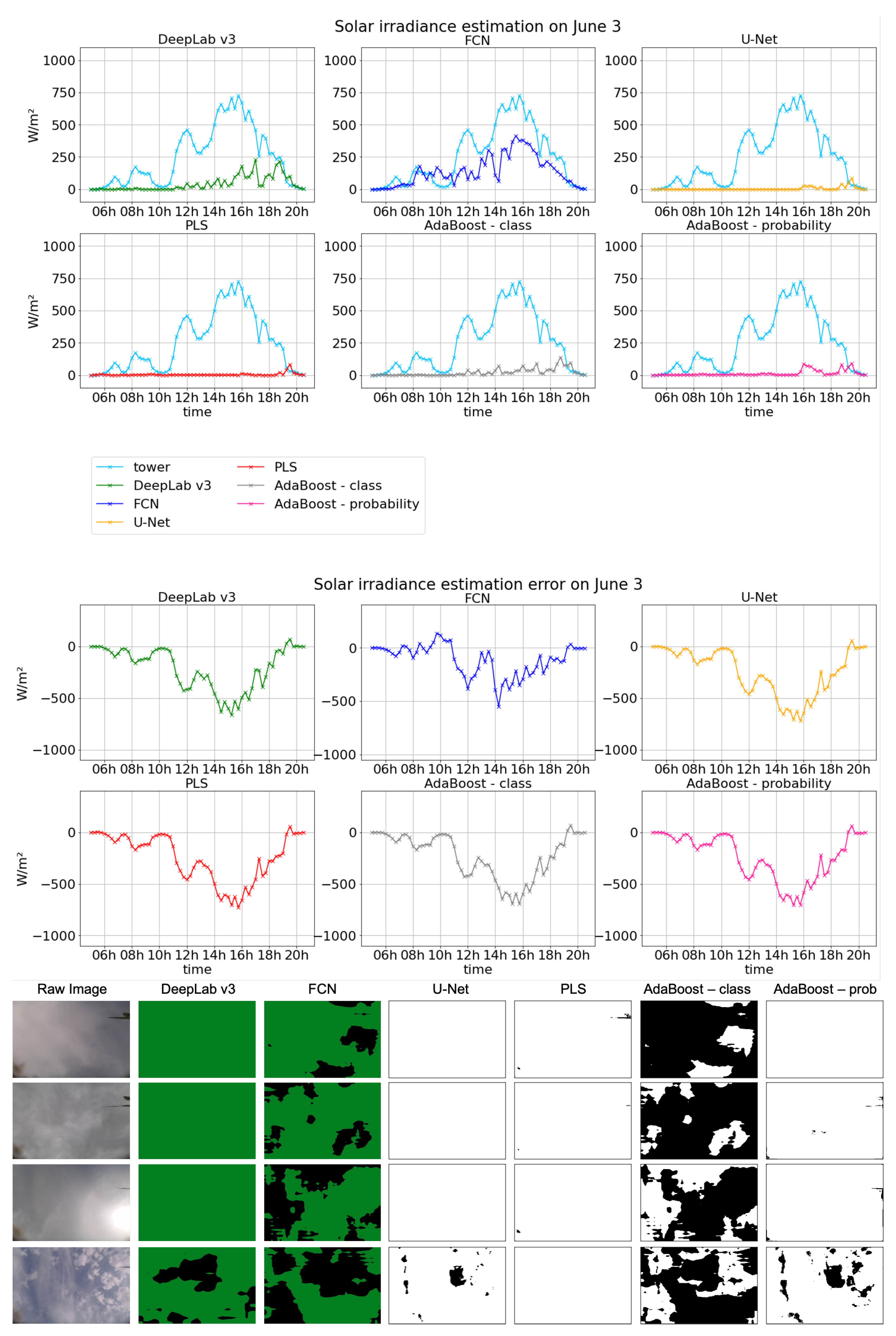
Appendix A.2.3. 3 June 2020

Figure A7. Solar irradiance estimation result based on cloud cover estimation from each machine learning model on 3 June 2020.
Atmosphere 12 00395 g0a7

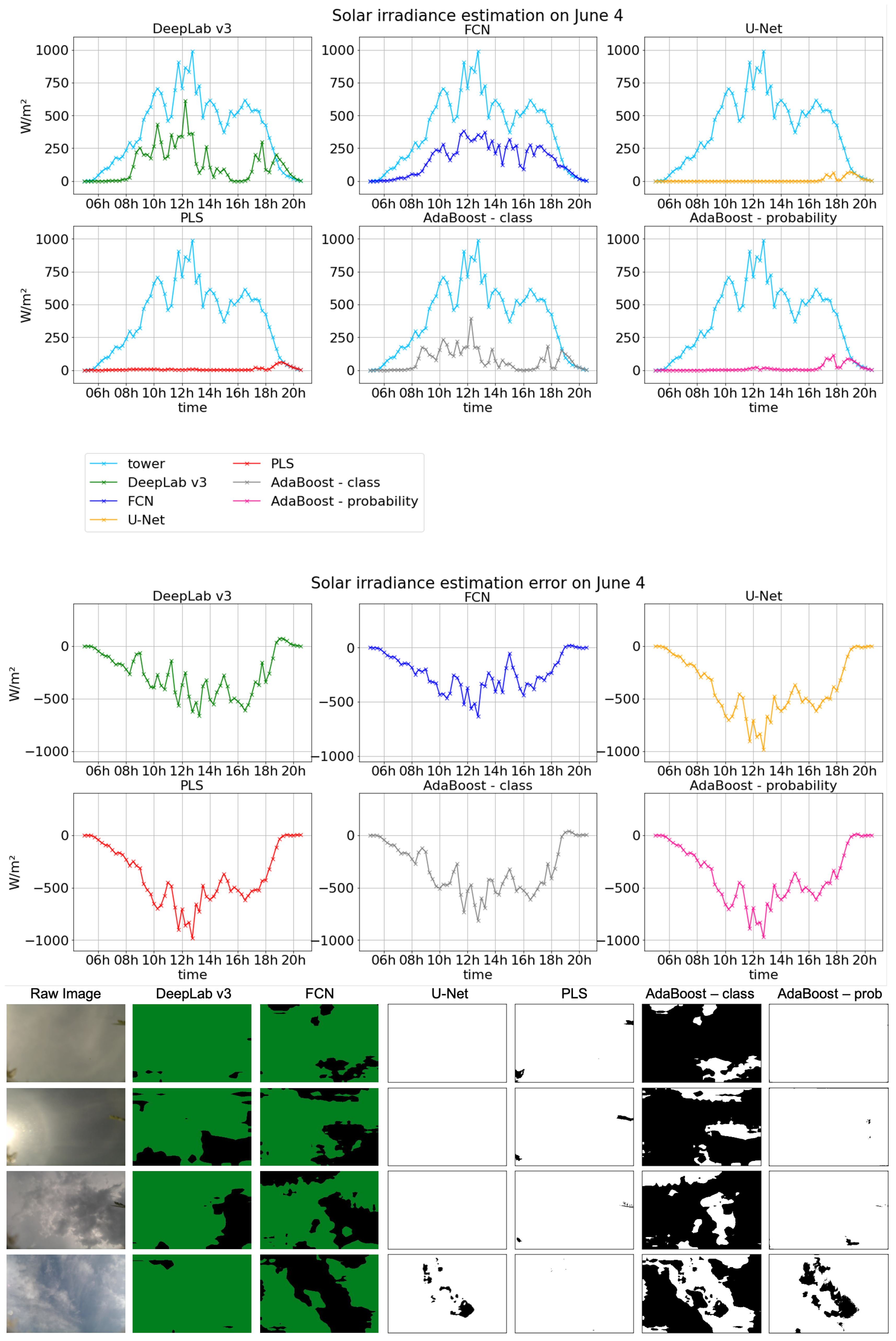
Appendix A.2.4. 4 June 2020

Figure A8. Solar irradiance estimation results based on cloud cover estimation from each machine learning model on 4 June 2020.
Atmosphere 12 00395 g0a8

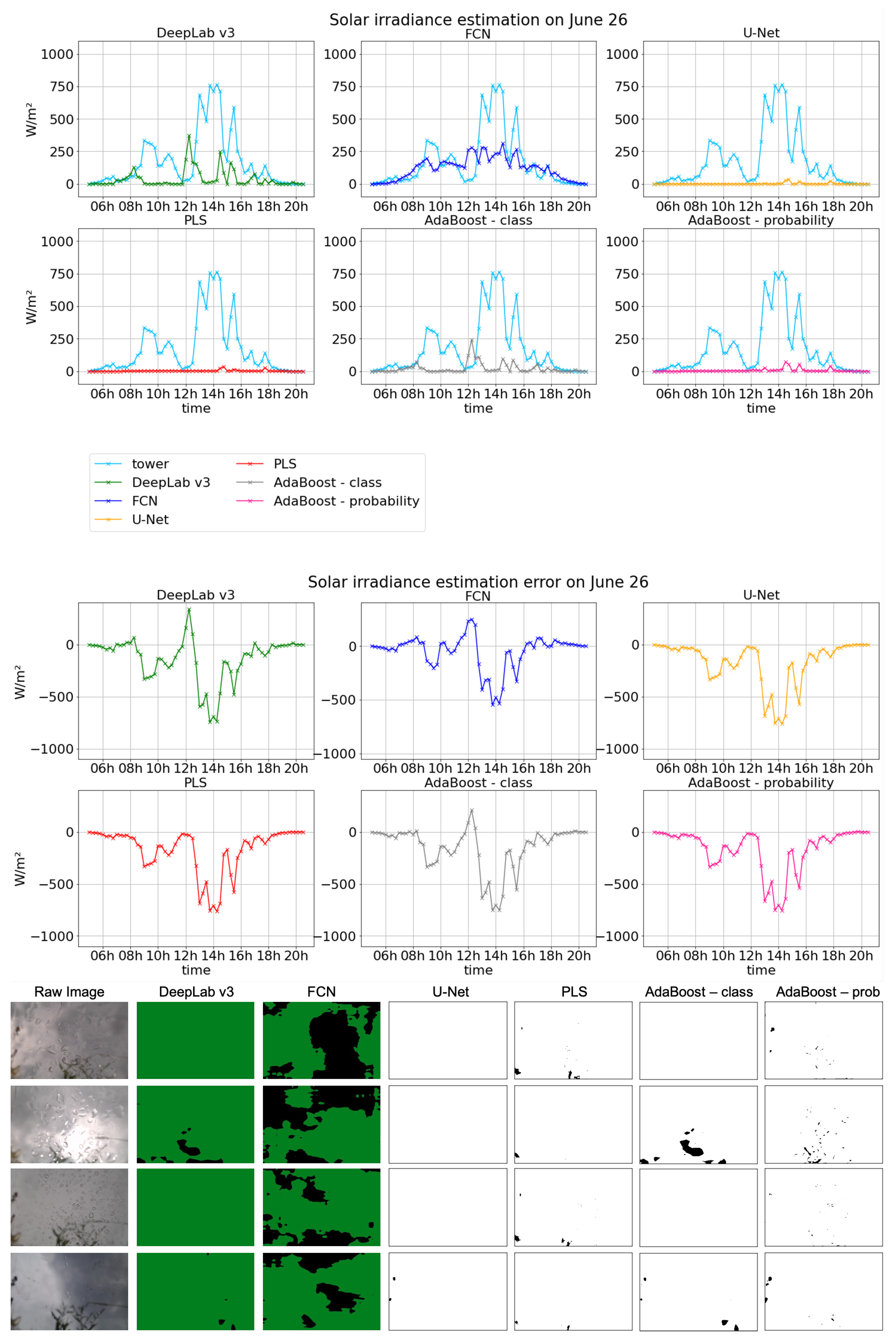
Appendix A.2.5. 26 June 2020

Figure A9. Solar irradiance estimation result based on cloud cover estimation from each machine learning model on 26 June 2020.
Atmosphere 12 00395 g0a9

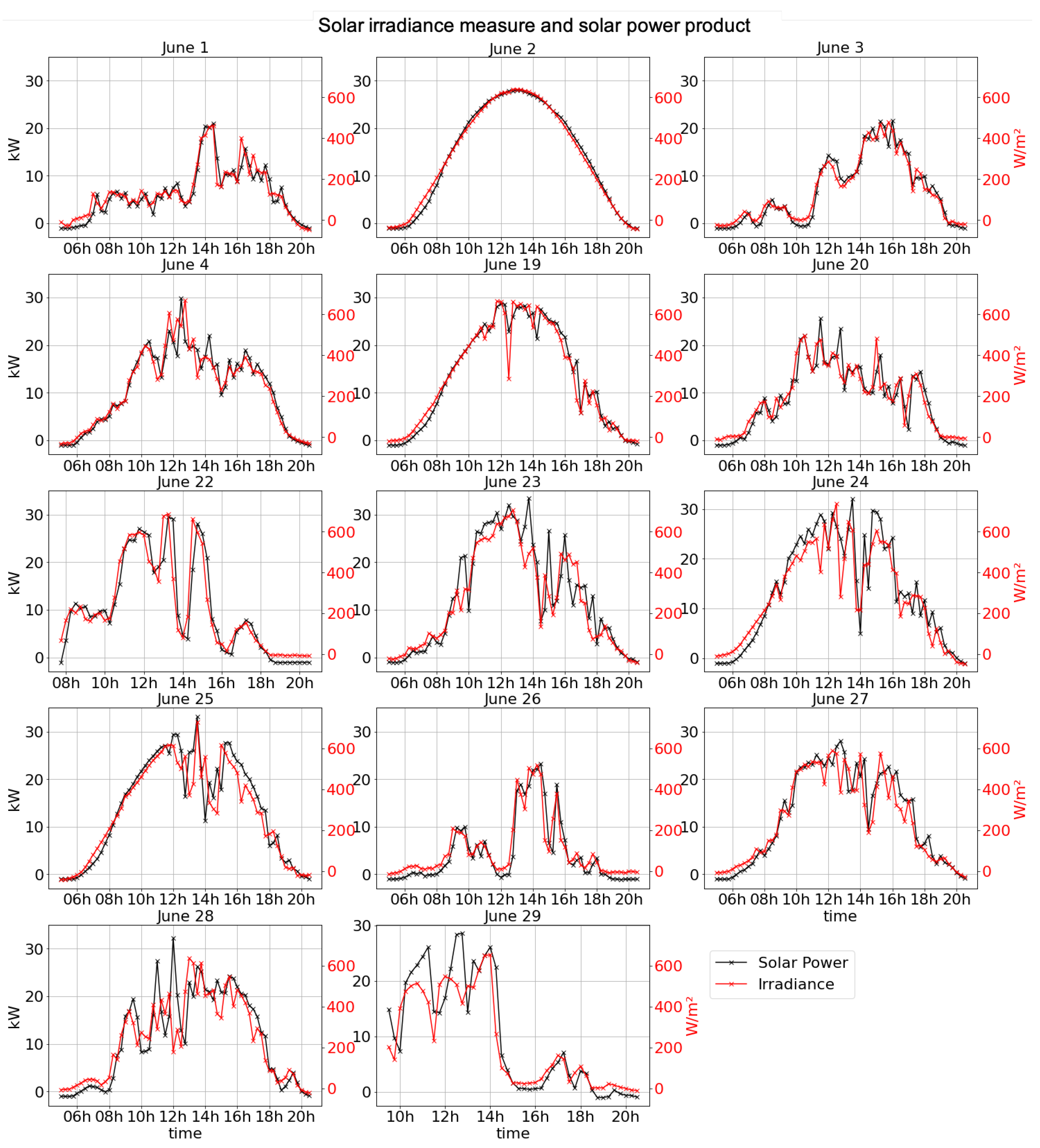
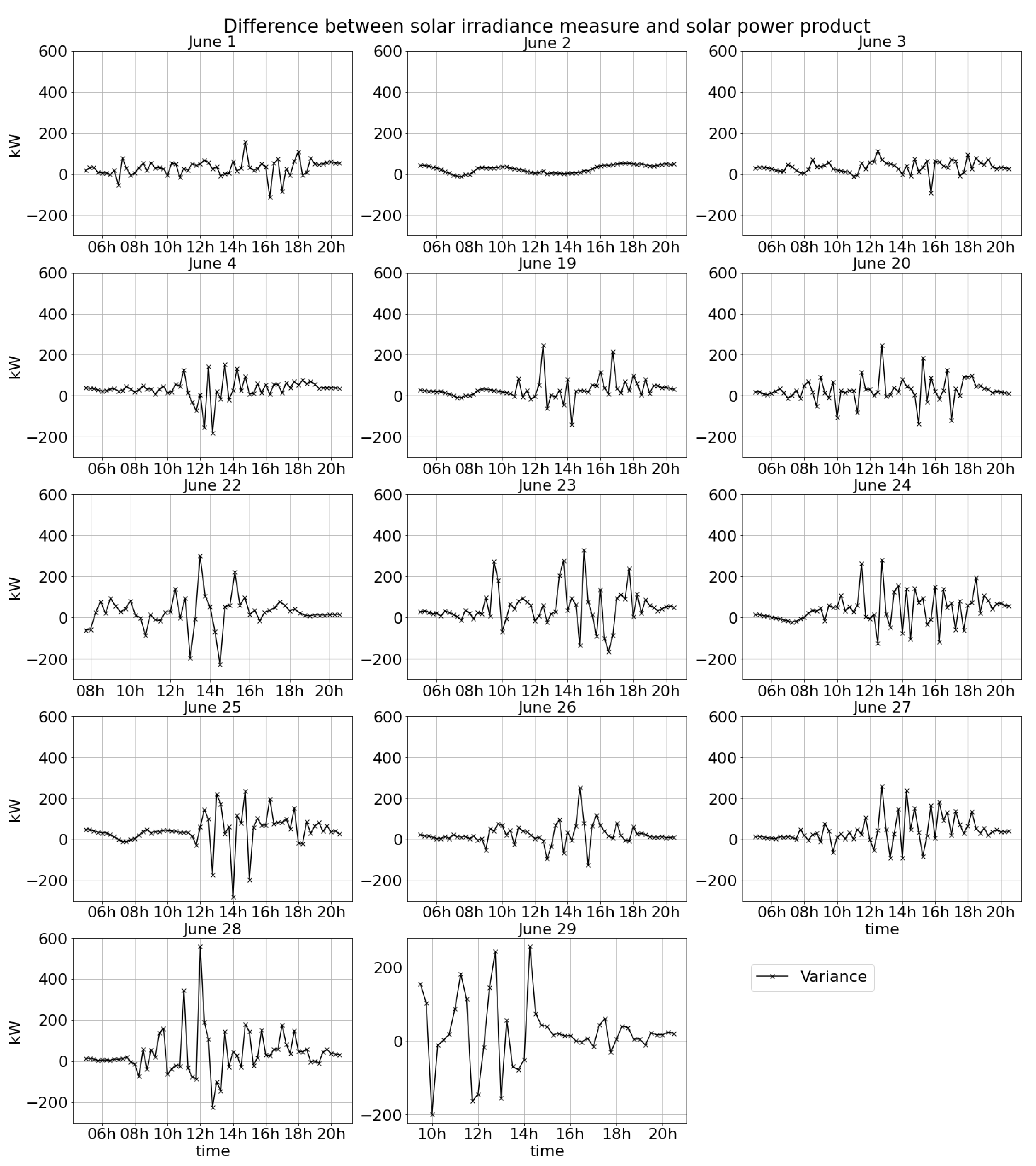
Appendix A.3. Comparison of Solar Irradiance Estimation and Solar Power Production Measure

Figure A10. Solar irradiance measure from the Argonne meteorological sensor tower and solar power product from the Argonne Energy Plaza for 14 days. The two locations are 1380 m apart in a straight line geographically.
Atmosphere 12 00395 g0a10
Figure A11. Difference between solar irradiance and solar power product when the solar power product is projected to the solar irradiance measure for 14 days.
Atmosphere 12 00395 g0a11

References

  1. Glotfelty, T.; Alapaty, K.; He, J.; Hawbecker, P.; Song, X.; Zhang, G. The Weather Research and Forecasting Model with Aerosol–Cloud Interactions (WRF-ACI): Development, Evaluation, and Initial Application. Mon. Weather Rev. 2019, 147, 1491–1511. [Google Scholar] [CrossRef] [PubMed]
  2. Illingworth, A.J.; Barker, H.; Beljaars, A.; Ceccaldi, M.; Chepfer, H.; Clerbaux, N.; Cole, J.; Delanoë, J.; Domenech, C.; Donovan, D.P. The EarthCARE satellite: The next step forward in global measurements of clouds, aerosols, precipitation, and radiation. Bull. Am. Meteorol. Soc. 2015, 96, 1311–1332. [Google Scholar] [CrossRef] [Green Version]
  3. Fu, C.L.; Cheng, H.Y. Predicting solar irradiance with all-sky image features via regression. Sol. Energy 2013, 97, 537–550. [Google Scholar] [CrossRef]
  4. Hollstein, A.; Segl, K.; Guanter, L.; Brell, M.; Enesco, M. Ready-to-use methods for the detection of clouds, cirrus, snow, shadow, water and clear sky pixels in Sentinel-2 MSI images. Remote Sens. 2016, 8, 666. [Google Scholar] [CrossRef] [Green Version]
  5. Zhu, Z.; Wang, S.; Woodcock, C.E. Improvement and expansion of the Fmask algorithm: Cloud, cloud shadow, and snow detection for Landsats 4–7, 8, and Sentinel 2 images. Remote Sens. Environ. 2015, 159, 269–277. [Google Scholar] [CrossRef]
  6. Wong, M.S.; Zhu, R.; Liu, Z.; Lu, L.; Peng, J.; Tang, Z.; Lo, C.H.; Chan, W.K. Estimation of Hong Kong’s solar energy potential using GIS and remote sensing technologies. Renew. Energy 2016, 99, 325–335. [Google Scholar] [CrossRef]
  7. Xie, F.; Shi, M.; Shi, Z.; Yin, J.; Zhao, D. Multilevel cloud detection in remote sensing images based on deep learning. IEEE J. Sel. Top. Appl. Earth Obs. Remote Sens. 2017, 10, 3631–3640. [Google Scholar] [CrossRef]
  8. Shi, M.; Xie, F.; Zi, Y.; Yin, J. Cloud detection of remote sensing images by deep learning. In Proceedings of the 2016 IEEE International Geoscience and Remote Sensing Symposium (IGARSS), Beijing, China, 10–15 July 2016; IEEE: Piscataway, NJ, USA, 2016; pp. 701–704. [Google Scholar]
  9. Chu, Y.; Pedro, H.T.; Li, M.; Coimbra, C.F. Real-time forecasting of solar irradiance ramps with smart image processing. Sol. Energy 2015, 114, 91–104. [Google Scholar] [CrossRef]
  10. Yang, H.; Kurtz, B.; Nguyen, D.; Urquhart, B.; Chow, C.W.; Ghonima, M.; Kleissl, J. Solar irradiance forecasting using a ground-based sky imager developed at UC San Diego. Sol. Energy 2014, 103, 502–524. [Google Scholar] [CrossRef]
  11. Chow, C.W.; Urquhart, B.; Lave, M.; Dominguez, A.; Kleissl, J.; Shields, J.; Washom, B. Intra-hour forecasting with a total sky imager at the UC San Diego solar energy testbed. Sol. Energy 2011, 85, 2881–2893. [Google Scholar] [CrossRef] [Green Version]
  12. Richardson, W.; Krishnaswami, H.; Vega, R.; Cervantes, M. A low cost, edge computing, all-sky imager for cloud tracking and intra-hour irradiance forecasting. Sustainability 2017, 9, 482. [Google Scholar] [CrossRef] [Green Version]
  13. Liu, S.; Zhang, L.; Zhang, Z.; Wang, C.; Xiao, B. Automatic cloud detection for all-sky images using superpixel segmentation. IEEE Geosci. Remote Sens. Lett. 2014, 12, 354–358. [Google Scholar]
  14. Marquez, R.; Gueorguiev, V.G.; Coimbra, C.F. Forecasting of global horizontal irradiance using sky cover indices. J. Sol. Energy Eng. 2013, 135, 011017. [Google Scholar] [CrossRef] [Green Version]
  15. Ghonima, M.; Urquhart, B.; Chow, C.; Shields, J.; Cazorla, A.; Kleissl, J. A method for cloud detection and opacity classification based on ground based sky imagery. Atmos. Meas. Tech. 2012, 5, 2881–2892. [Google Scholar] [CrossRef] [Green Version]
  16. Kazantzidis, A.; Tzoumanikas, P.; Bais, A.F.; Fotopoulos, S.; Economou, G. Cloud detection and classification with the use of whole-sky ground-based images. Atmos. Res. 2012, 113, 80–88. [Google Scholar] [CrossRef]
  17. Li, Q.; Lu, W.; Yang, J. A hybrid thresholding algorithm for cloud detection on ground-based color images. J. Atmos. Ocean. Technol. 2011, 28, 1286–1296. [Google Scholar] [CrossRef]
  18. Dev, S.; Lee, Y.H.; Winkler, S. Color-based segmentation of sky/cloud images from ground-based cameras. IEEE J. Sel. Top. Appl. Earth Obs. Remote Sens. 2016, 10, 231–242. [Google Scholar] [CrossRef]
  19. Dev, S.; Lee, Y.H.; Winkler, S. Systematic study of color spaces and components for the segmentation of sky/cloud images. In Proceedings of the 2014 IEEE International Conference on Image Processing (ICIP), Paris, France, 27–30 October 2014; IEEE: Piscataway, NJ, USA, 2014; pp. 5102–5106. [Google Scholar]
  20. Moncada, A.; Richardson, W.; Vega-Avila, R. Deep learning to forecast solar irradiance using a six-month UTSA skyimager dataset. Energies 2018, 11, 1988. [Google Scholar] [CrossRef] [Green Version]
  21. Zhang, J.; Liu, P.; Zhang, F.; Song, Q. CloudNet: Ground-based cloud classification with deep convolutional neural network. Geophys. Res. Lett. 2018, 45, 8665–8672. [Google Scholar] [CrossRef]
  22. Drönner, J.; Korfhage, N.; Egli, S.; Mühling, M.; Thies, B.; Bendix, J.; Freisleben, B.; Seeger, B. Fast cloud segmentation using convolutional neural networks. Remote Sens. 2018, 10, 1782. [Google Scholar] [CrossRef] [Green Version]
  23. Li, X.; Lu, Z.; Zhou, Q.; Xu, Z. A Cloud Detection Algorithm with Reduction of Sunlight Interference in Ground-Based Sky Images. Atmosphere 2019, 10, 640. [Google Scholar] [CrossRef] [Green Version]
  24. Flickr. Available online: https://www.flickr.com (accessed on 11 February 2021).
  25. Onishi, R.; Sugiyama, D. Deep convolutional neural network for cloud coverage estimation from snapshot camera images. SOLA 2017, 13, 235–239. [Google Scholar] [CrossRef] [Green Version]
  26. Long, J.; Shelhamer, E.; Darrell, T. Fully convolutional networks for semantic segmentation. In Proceedings of the IEEE conference on computer vision and pattern recognition, Boston, MA, USA, 7–12 June 2015; pp. 3431–3440. [Google Scholar]
  27. Ronneberger, O.; Fischer, P.; Brox, T. U-Net: Convolutional networks for biomedical image segmentation. In Proceedings of the International Conference on Medical Image Computing and Computer-Assisted Intervention, Munich, Germany, 5–9 October 2015; Springer: New York, NY, USA, 2015; pp. 234–241. [Google Scholar]
  28. Chen, L.C.; Papandreou, G.; Schroff, F.; Adam, H. Rethinking atrous convolution for semantic image segmentation. arXiv 2017, arXiv:1706.05587. [Google Scholar]
  29. Keahey, K.; Mambretti, J.; Ruth, P.; Stanzione, D. Chameleon: A Large-Scale, Deeply Reconfigurable Testbed for Computer Science Research. In Proceedings of the 2019 IEEE 27th International Conference on Network Protocols (ICNP), Chicago, IL, USA, 8–10 October 2019; IEEE: Piscataway, NJ, USA, 2019; pp. 1–2. [Google Scholar]
  30. Chameleonurl. Available online: https://www.chameleoncloud.org (accessed on 11 February 2021).
  31. Chen, L.C.; Zhu, Y.; Papandreou, G.; Schroff, F.; Adam, H. Encoder-decoder with atrous separable convolution for semantic image segmentation. In Proceedings of the European Conference on Computer Vision (ECCV), Munich, Germany, 8–14 September 2018; Springer: New York, NY, USA, 2018; pp. 801–818. [Google Scholar]
  32. Chen, L.C.; Papandreou, G.; Kokkinos, I.; Murphy, K.; Yuille, A.L. DeepLab: Semantic image segmentation with deep convolutional nets, atrous convolution, and fully connected CRFs. IEEE Trans. Pattern Anal. Mach. Intell. 2017, 40, 834–848. [Google Scholar] [CrossRef] [PubMed]
  33. He, K.; Zhang, X.; Ren, S.; Sun, J. Spatial pyramid pooling in deep convolutional networks for visual recognition. IEEE Trans. Pattern Anal. Mach. Intell. 2015, 37, 1904–1916. [Google Scholar] [CrossRef] [PubMed] [Green Version]
  34. Krähenbühl, P.; Koltun, V. Efficient inference in fully connected CRFs with Gaussian edge potentials. In Advances in Neural Information Processing Systems; MIT Press: Cambridge, MA, USA, 2011; pp. 109–117. [Google Scholar]
  35. Schapire, R.E. Explaining AdaBoost. In Empirical Inference; Springer: New York, NY, USA, 2013; pp. 37–52. [Google Scholar]
  36. Beckman, P.; Sankaran, R.; Catlett, C.; Ferrier, N.; Jacob, R.; Papka, M. Waggle: An open sensor platform for edge computing. In Proceedings of the 2016 IEEE SENSORS, Orlando, FL, USA, 30 October–3 November 2016; IEEE: Piscataway, NJ, USA, 2016; pp. 1–3. [Google Scholar]
  37. Metower. Available online: https://www.atmos.anl.gov/ANLMET/index.html (accessed on 11 February 2021).
  38. Plaza. Available online: https://dashboard.ioc.anl.gov/viewer.html?proj=Argonne (accessed on 11 February 2021).
  39. Martins, F.; Silva, S.; Pereira, E.; Abreu, S. The influence of cloud cover index on the accuracy of solar irradiance model estimates. Meteorol. Atmos. Phys. 2008, 99, 169–180. [Google Scholar] [CrossRef]
  40. Lengfeld, K.; Macke, A.; Feister, U.; Güldner, J. Parameterization of solar radiation from model and observations. Meteorol. Z. 2010, 19, 25–33. [Google Scholar] [CrossRef] [Green Version]
  41. Badescu, V.; Dumitrescu, A. New types of simple non-linear models to compute solar global irradiance from cloud cover amount. J. Atmos. Sol. Terr. Phys. 2014, 117, 54–70. [Google Scholar] [CrossRef]
  42. Beckman, P.; Catlett, C.; Altintas, I.; Kelly, E.; Collis, S. Mid-Scale RI-1: SAGE: A Software-Defined Sensor Network (NSF OAC 1935984). 2019. Available online: https://sagecontinuum.org/ (accessed on 11 February 2021).
Figure 1. Data-processing flow for cloud cover measure and solar irradiance estimation.
Atmosphere 12 00395 g001
Figure 2. Example images and corresponding labels from the Waggle cloud dataset. The original image resolution was 2304 × 1536, resized to 300 × 300 to improve computational performance during the training process (see Section 2). The sky pixels were identified by the two-step process described in Section 3.3.
Atmosphere 12 00395 g002
Figure 3. Cloud segmentation results from the six machine learning models along with input and ground truth images. From the right, the images are input; ground truth; and results from DeepLab v3, FCN, U-Net, PLS, AdaBoost trained with class number, and AdaBoost trained with normalized cloud probability.
Atmosphere 12 00395 g003
Figure 4. Results of 15 min averaged cloud cover estimation. The results show ratios of cloud pixels in images at each time point. If no cloud pixel was detected, the ratio was calculated as 0; if the whole sky was covered with cloud, the ratio was calculated as 1. The results are shown for the cloud types (a) clear sky, (b,c) haze clouds, (d) partially cloudy sky, and (e) overcast.
Atmosphere 12 00395 g004
Figure 5. Measured solar irradiance (light blue) and solar irradiance estimation results in W/m 2 using 15 min averaged cloud cover estimation and maximum solar irradiance measured on 2 June 2020 for five days with (a) clear sky, (b,c) haze clouds, (d) partially cloudy sky, and (e) overcast clouds. The tower measure on 2 June ( b l u e l i n e ) is overlapped with the DeepLab v3 estimation results ( g r e e n l i n e ), with only a small difference between these observable at 7–8 h.
Atmosphere 12 00395 g005
Figure 6. Solar irradiance estimation error in W/m 2 . The results are shown for the cloud types (a) clear sky, (b,c) haze clouds, (d) partially cloudy sky, and (e) overcast.
Atmosphere 12 00395 g006
Figure 7. Solar irradiance measure from the Argonne meteorological sensor tower and solar power product from the Argonne Energy Plaza. The two locations are 1380 m apart in a straight line geographically. The results are shown for the cloud types (a) clear sky, (b,c) haze clouds, (d) partially cloudy sky, and (e) overcast.
Atmosphere 12 00395 g007
Figure 8. Difference between solar irradiance and solar power product when the solar power product is projected to the solar irradiance measure. The results are shown for the cloud types (a) clear sky, (b,c) haze clouds, (d) partially cloudy sky, and (e) overcast.
Atmosphere 12 00395 g008
Table 1. Segmentation accuracy of each model. The validation of the models was performed with a dataset consisting of selected images from the Hybrid Thresholding Algorithm (HYTA) and Singapore Whole Sky Imaging Segmentation (SWIMSEG).
ModelmIoUmAPmAR
PLS0.64670.89610.6991
FCN0.56490.89740.6040
U-Net0.76260.98690.7703
DeepLab0.53350.92340.5582
AdaBoost (class)0.61280.84940.6875
AdaBoost (probability)0.58560.86460.6448
Table 2. Number of images selected each day.
Date6/16/26/36/46/196/206/22
Number of Images3776377337633759383737613058
Date6/236/246/256/266/276/286/29
Number of Images3777375737783775377137592639
Table 3. Overall error rate in percentage and root mean square error (RMSE) on estimating solar irradiance.
ModelMean Error (%)RMSE (W/m 2 )
ClearPartially CloudyCloudyClearPartially CloudyCloudy
FCN48.7556.9454.60296.19300.02219.16
U-Net21.8169.4392.88152.64357.84367.88
PLS42.6976.9093.22269.89404.02367.97
DeepLab0.2233.8262.574.09142.83295.47
AdaBoost (class)12.0160.4788.2225.77208.90328.25
AdaBoost (probability)3.5844.3074.8988.18292.71360.50
Publisher’s Note: MDPI stays neutral with regard to jurisdictional claims in published maps and institutional affiliations.

