Comparative Analysis between Daily Extreme Temperature and Precipitation Values Derived from Observations and Gridded Datasets in North-Western Romania

Abstract

Climate gridded datasets are highly needed and useful in conducting data analysis for research and practical purposes. They provide long-term information on various climatic variables for large areas worldwide, making them suitable for use at any spatial level. It is essential to assess the accuracy of gridded data by comparing the data to measured values, especially when they are used as input parameters for hydro-climatic models. From the multitude of databases available for North-western Romania, we selected three, particularly the European Climate Assessment and Dataset (E-OBS), the Romanian Climatic Dataset (ROCADA), and the Climate of the Carpathian Region (CARPATCLIM). In this paper, we analyse the extreme precipitation and temperature data derived from the above-mentioned datasets over a common 50-year period (1961–2010) and compare the data with raw values to estimate the degree of uncertainty for each set of data. The observation data, recorded at two meteorological stations located in a complex topography region, were compared to the output of the gridded datasets, by using descriptive statistics for the mean and extreme annual and seasonal temperature and precipitation data, and trend analyses. The main findings are: the high suitability of the ROCADA gridded database for climate trend analysis and of the E-OBS gridded database for extreme temperature and precipitation analysis.

1. Introduction

Extremely useful in various stages of research and data analysis, daily gridded datasets are increasingly used as climatic parameter input for modelling, statistical analysis of time series, trend analysis, etc. [1,2]. They have the advantage of being able to cover large areas and, by various homogenization and interpolation methods, can be successfully used as input parameters in many climatic/hydrological models or for different types of analysis based on time series [3,4,5].

No matter what domain they are employed in, some important questions arise. How reliable and accurate are these datasets and what types of analysis are they suitable for? Can they be used to determine climate change or as input data for hydrological modelling? How does one choose from the multitude of gridded datasets available for a focus region, i.e., which one is the most appropriate for a specific study? Usually, one of the most common approaches is to select those gridded datasets that provide the values closest to the observed values in the area under study, and therefore are the most suitable for further analysis.

However, considering their advantages and availability, gridded datasets require a thorough examination for validation before use, by comparing estimations with observation data [6]. To fill the gaps in the available datasets generated by inconsistencies in data collection and recording [7], researchers have focused on creating and testing various methodologies resulting in replicable models of data reconstruction and increased quality control.

The need for datasets to be as accurate and complete as possible is strongly argued by numerous researchers worldwide, since any gaps, errors, and particular characteristics of datasets and recordings of climate data bring challenges in delivering high-quality end results [7,8,9,10,11,12]. However, studies have revealed significant gaps in the data needed; sometimes, there have been no correlation achieved within the recorded data [7], or there have been many inconsistencies and low correlation between the information provided by the datasets and those recorded at in situ stations, especially in the case of long-term data [11,12,13].

Good quality data have become a priority since they are a prerequisite for different types of scientific studies. Using various statistical metrics, researchers have tested the accuracy of available datasets providing daily and monthly data at a global or regional level, on different climatic variables, in order to prove their suitability for practical applications in hydrological modelling, monitoring of climatic extreme events, or environmental studies [7,8,9,11,14]. Thus, a tool has been developed for creating custom datasets from observed daily precipitation records using the reddPrec package, an open source R package, which can be replicated by researchers in their attempts to create and use a suitable and distinct database adapted to their needs [15].

A number of gridded dataset studies, developed by specialists worldwide, have focused on data series that cover large areas, in which case topographic complexity is less important. Usually, the analysed periods of estimated data availability in multiple datasets vary from 20 to 50 years. Results have shown that researchers prefer to perform studies by using certain climate gridded datasets, after analysing them comparatively and in accordance with the value of correlation between estimated and observation data [6,9,11,12,13,14,16]. Some others have focused on interpolation methods and data homogenization for validation [1,3,4,5,17].

In Romania, some authors have examined the climate-growth relationship of oak trees in the South Carpathians based on daily and monthly precipitation and temperature data, over a 50-year period, provided by the following three climate gridded databases: Climatic Research Unit TimeSeries (CRU TS), European Climate Assessment and Dataset (E-OBS), and RomanianClimatic Dataset (ROCADA). The results have shown differences between the data provided by the three climate products, arguing for selective suitability regarding the use of the ROCADA and E-OBS databases in relation to the specific purposes of researchers when performing dendroclimatological and dendroecological studies [16].

Climate information has proven to be highly significant for advancement in research in various fields, such as hydrology [7], energy sector [8], dendroclimatology and dendroecology [16], environment, and for understanding and monitoring natural hazards and hydrological cycle characteristics [11]. Moreover, good quality climate data is of crucial importance for developing performant products and climate services and their selection is decisive in providing reliable climate projections and scenarios. Furthermore, they are used as tools for future impact studies employed to set up policies and strategies for climate change adaptation and mitigation [10]. A qualitative study based on structured and semi-structured interviews has revealed the climate information that is needed across socioeconomic sectors in Europe for climate change adaptation and risk mitigation [18]. The authors have emphasized the opportunity of using the available data and providing climate products and services to enhance knowledge on climate change, which is of the essence for decision-makers when they customize policies for the support of end users. All along, some authors have argued that there is a need for accurate climate information so that measures and policies adopted for the energy sector regarding adaptation to climate variability and change would be the most efficient. They have identified several issues encountered when using climate datasets for this purpose, which included heterogeneity of available information, differences in time and spatial resolution, types of access and available platforms as well as bias of models [8].

For North-western Romania, a multitude of daily gridded datasets are available for different climatic parameters, but which one to choose still remains difficult. For the complex topography area in North-western Romania, only one study has been conducted [1] that has compared the string values of a gridded dataset with the observed values, yet, without targeting the locations under analysis. Nevertheless, there are many studies that have used different databases without prior validation [19,20,21]. In the presentation of ROCADA, there has been a comparison developped among its resulting datasets, and those returned by E-OBS and APHRODITE, considering the observation values recorded at six meteorological stations randomly distributed across the entire territory of Romania [1].

The main purpose of this study is to determine which datasets (from the available ones) are the most suitable for use at a very small spatial scale, in a complex topography area. When considering gridded datasets for larger regions, the topography “details” seem to be smoothened, but for small areas and communities, it is essential to choose the best datasets (in terms of accuracy and spatial resolution) as the impact of extreme events could be significant. This study is part of a wider research project aiming at determining the impact of climate change on river discharge flows in North-western Romania. One of the most important issues of such a research topic in a complex topography region is the accuracy of the climate data to be used as input for hydrological modelling. In this general context, we compared the gridded datasets derived from three databases with the observation data to select the most appropriate one to be further employed in a hydrological modelling study.

2. Materials and Methods

2.1. Data Used

To perform the comparison of the selected datasets, daily observation data recorded at two meteorological stations (Baia Mare and Ocna Șugatag) located in a region with complex topography were considered and compared with data derived from the following three databases: ROCADA [1], E-OBS [22,23], and Climate of the Carpathian Region (CARPATCLIM) [24]. Both weather stations belong to the National Meteorological Administration (NMA) network in Romania. Their location is presented in Figure 1 and their geographical coordinates in

Table 1. The geographical coordinates of the meteorological stations.

Meteorological Stations	Longitude (°)	Latitude (°)	Altitude (m)
Ocna Șugatag	23.94214	47.77737	503
Baia Mare	23.49324	47.66121	196

.

The following climatic parameters were used for comparison: daily data of maximum temperature (TX), minimum temperature (TN), and precipitation (RR). Data strings corresponding to a common 50-year reference period (1961–2010) were employed for both observation and gridded data.

2.1.1. Observation Data

Most of the daily extreme temperature and precipitation data were freely downloaded from the European Climate Assessment and Dataset (ECA&D) project database (non-blended data) for the period 1961–2009 [22,23] and reconstructed from raw synoptic messages available on www.meteomanz.com (accessed on 16 February 2016) for the year 2010 [25].

As described on www.ecad.eu (accessed on 23 March 2020), “the non-blended series are the series as provided by the participants: the climate variable series collected from participating countries generally do not contain data for the most recent years. This is partly due to the time that is needed for data quality control and archiving at the home institutions of the participants, and partly the result of the efforts required to include the data in the ECA database. To make available for each station a time series that is as complete as possible, an automated update procedure has been included that relies on the daily data from SYNOP messages that are distributed in near real time over the Global Telecommunication System (GTS). By using this procedure, the gaps in a daily series were filled in with observations from nearby stations, provided that they are within 12.5 km distance and that height differences are less than 25 m”, and thus the blended data series were derived [23]. Under these circumstances, for this study and for a more accurate analysis, we chose the non-blended data series.

The observation datasets were reconstructed and tested for homogeneity under the framework of the FMETPRO project (http://fmetpro.granturi.ubbcluj.ro, accessed on 28 March 2020) on extreme weather events related to temperature and precipitation in Romania [25].

2.1.2. Gridded Data

Data extracted from three databases were analysed:

i. The ROCADA database, developed by the NMA, provides daily data for a 53-year period (1961–2013) for the entire territory of Romania. For homogenization and interpolation, 155 meteorological stations for TX and TN, and 188 meteorological stations for precipitation were employed. It has a spatial resolution of 0.1° × 0.1° (~11 km × 11 km) (Figure 2a). Datasets are freely available on the World Data Centre PANGAEA portal [1]. The homogenization was performed by using the MASH method, whereas for interpolation, the MISH procedure was employed; both methods are described in detail in [1,17,26,27,28]. The same methods were previously successfully used for creating the CARPATCLIM project database [24,26,27,28,29].

None of the considered stations for the present study was used for the validation of the ROCADA database.

ii. The CARPATCLIM database, developed under the framework of the project Climate of the Carpathian Region [24,26], covers an area of 483,525 km² and a 50-year period (1961–2010). As presented on the project website, it was developed by interpolating observation data from 585 precipitation and meteorological stations for the entire region. For Romania’s territory, 67 stations were used for gridding precipitation and 91 stations for gridding TX and TN over Romania. To obtain the grid values, spatial interpolation was performed at the national level, using MISH/MASH software [17,26,27,28,29] and afterwards, compiled at the CARPATCLIM region level. Between the neighbouring countries, the near-border station data series were exchanged to cross-border harmonize the interpolation [24,26]. Data are freely available on the website of the project (http://www.carpatclim-eu.org, accessed on 15 January 2020). The spatial resolution of the grid is 0.1° × 0.1° (~11 km × 11 km) (Figure 2b). None of the considered stations for the present study was used to validate the database.

iii. The E-OBS is a database developed at the European level and contains 54,095 series of observations for 12 elements recorded at 15,562 meteorological stations throughout Europe, over the period 1950–2019. From Romania, data recorded at 27 weather stations for extreme temperatures and 28 weather stations for precipitation were considered for interpolation. The E-OBS comes as an ensemble dataset and is available on a 0.1° regular grid (~11 km × 11 km) (Figure 2c). The dataset is constructed based on a conditional simulation procedure. For each of the members of the ensemble, a spatially correlated random field is produced using a predetermined spatial correlation function. The mean across members is calculated and is provided as the “best-guess” field. The spread is calculated as the difference between the 5th and the 95th percentiles over the ensemble to provide a measure indicating the 90% uncertainty range [22,23,30].

All gridded datasets used in this study are freely available on the project’s website (www.ecad.eu, accessed on 23 March 2020), to be used for non-commercial research projects, upon request.

For further analysis, a common 50-year period, 1961–2010, for all datasets considered was employed.

2.2. Methods

The time series derived from each gridded dataset were extracted based on the geographical coordinates of the weather stations, by intersection. For this task, we used ArcGIS Pro software (multidimension tools) (produced by ESRI, Redlands, CA, USA), by overlapping the point-type layer (used for the location of the meteorological stations) with each gridded dataset. Because the centre of the grid does not coincide with the location of the station, we used the nearest neighbourhood method to extract the data. Starting from the considered data strings and having observation data as reference values, four main categories of analysis were further performed, as described below.

2.2.1. Descriptive Statistics

In the first category, descriptive statistics were performed for both observation and gridded data series to be able to identify the differences between them. Afterwards, Pearson’s correlation coefficient and the coefficient of determination (R-squared) were calculated for the pairs consisting of observation data and each gridded data series for the three parameters considered.

2.2.2. Comparison between the Extreme Values Derived from Gridded Datasets and from Observations Using the Complete Datasets

The second category of analysis focused on the comparison between the extreme values derived from gridded datasets and the results from observations. The extreme percentile (the 1st and the 99th) values and the extreme annual values were both considered as follows: (i) from each gridded dataset, all values equal to or lower than the 1st percentile and values equal to or greater than the 99th percentile were extracted and compared with the corresponding values derived from the observation datasets and (ii) the extreme annual values from each gridded dataset were selected and compared with the observed ones.

The datasets obtained based on the extreme percentile values were further analysed by using Taylor diagrams and the coefficient of determination. Taylor diagrams are mathematical diagrams especially developed to graphically indicate which of the models of a system, dataset, process, or phenomenon is located closest to a reference value (observation value, in this case). This type of diagram, designed by Karl E. Taylor in 1994 and published in 2001 [31], allows for a comparative evaluation of different models. For this study, it was used to assess the degree of similarity between the values of the gridded (modelled) datasets and the reference one (observation-derived dataset) using the following three statistical indices: Pearson’s correlation coefficient, root mean square error (RMSE), the standard deviation. The Taylor diagrams provide a concise statistical summary of how well patterns match each other in terms of their correlation, their root mean square difference, and the ratio of their variances [31]. They allow simultaneous visualization of the three statistical parameters over the three gridded datasets as compared with the observation ones for each location. An R package was employed to create the diagrams.

The coefficient of determination allows the indication of the data points scattered around the regression line, both for the percentile and for the annual extreme values series.

2.2.3. Comparison between Seasonal Values Derived from Gridded Datasets and from Observations

The third category of analysis involved extracting and comparing the seasonal values related to the extreme seasons, winter (December, January, and February) and summer (June, July, and August), corresponding to each dataset. The analysis of the relation between the databases according to seasons was performed by applying the following approaches:

i. A comparative analysis of two distributions by Kolmogorov–Smirnov test (K-S) [32]. This analysis shows the absolute maximum distance between two distributions of the time series with observed values as compared with the values of the gridded dataset;

ii. An analysis of seasonal datasets using Taylor diagrams to quantify the degree of correspondence between the modelled and the observed behaviour in terms of three statistical indicators, i.e., Pearson’s correlation coefficient, RMSE, and standard deviation [30].

2.2.4. Trend Analysis

The analysis of TX, TN, and RR temporal evolution was approached by employing a combination of the Mann–Kendall test for trends [33,34] with Sen’s non-parametric method for the magnitude of the trend [35]. The combined method is widely used to detect changes in different climatic parameter datasets [36,37,38,39]. The Mann–Kendall test can be applied to detect a monotonic trend of a time data series, whereas Sen’s method uses a linear model to estimate the slope of the trend, while the variance of the residuals should be constant in time [40].

3. Results and Discussions

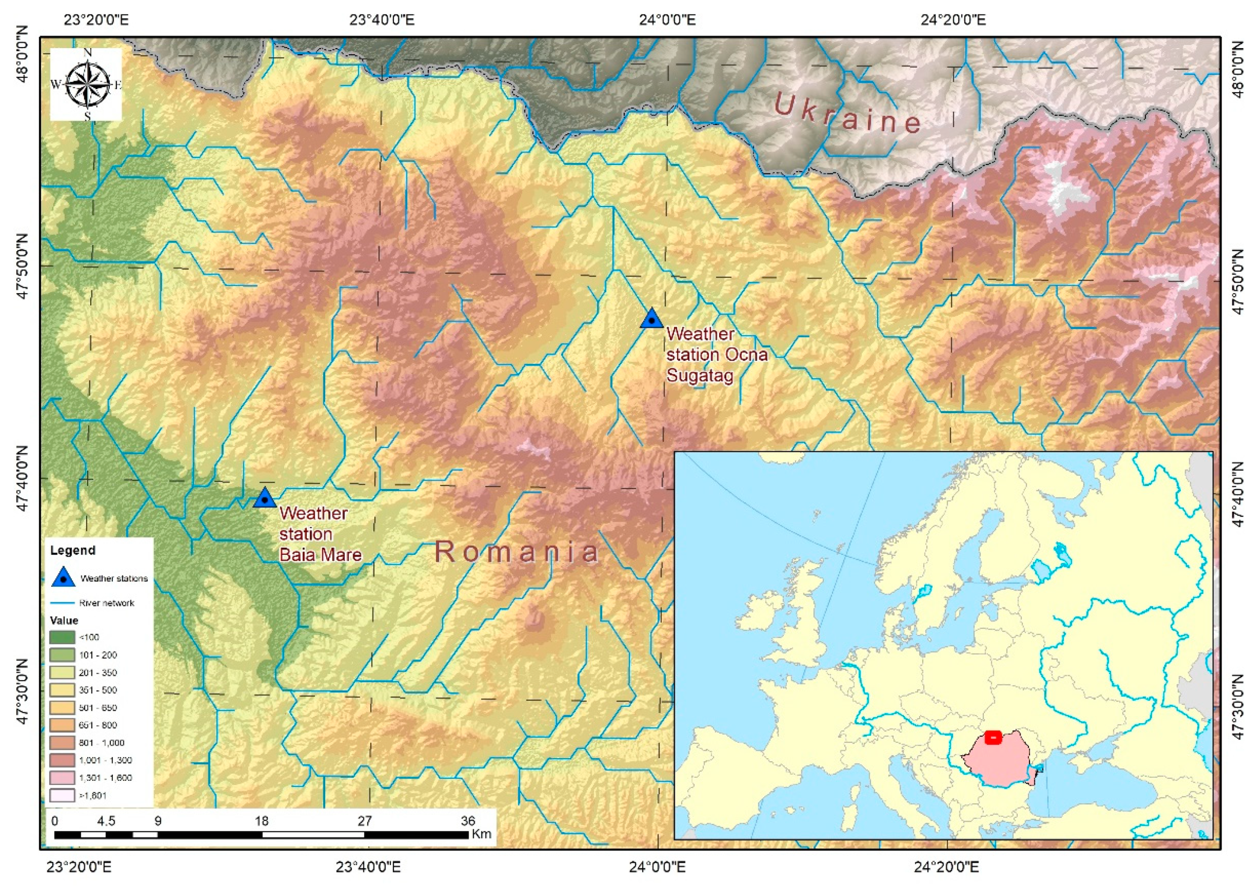
3.1. Study Region

The focus region is small, but it has a complex topography; the selected area extends over two mountain depressions developed on opposite sides of the Țibleș Mountains. Although territorially close to each other, their general climate features are quite different due to their altitude and the barrier generated by the presence of mountains between them. The Meteorological Station of Baia Mare is located in the Baia Mare Depression, on the western side of the mountain chain (Figure 1). This area is characterized by a total annual amount of precipitation of 884 mm/year and by a mean multiannual temperature of 9.6 °C. It is widely open westward and the dominant air masses originate over the North Atlantic Ocean. The Meteorological Station of Ocna Șugatag is located in the Maramureș Depression, East of the Țibleș Mountains (Figure 1). The recorded annual precipitation and mean multiannual temperature are considerably lower than those of Baia Mare (746 mm and 6.8 °C).

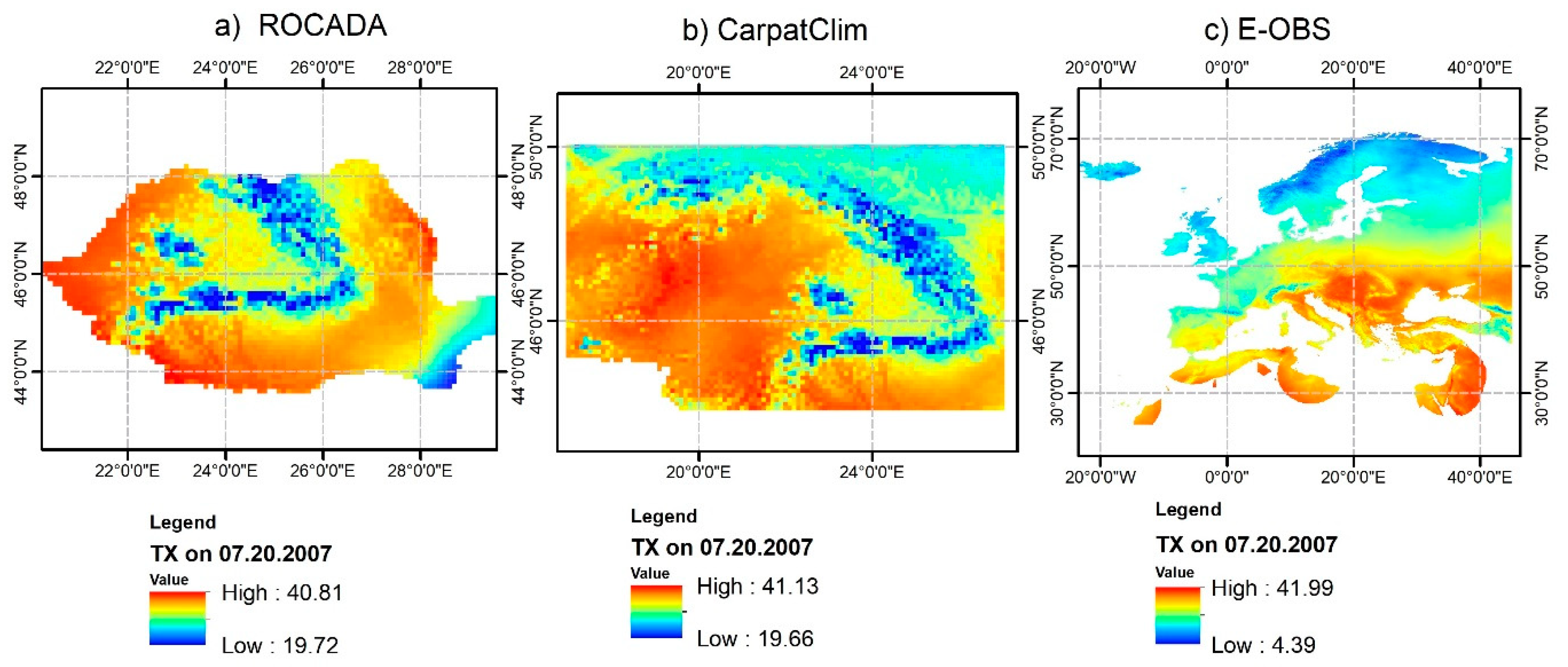
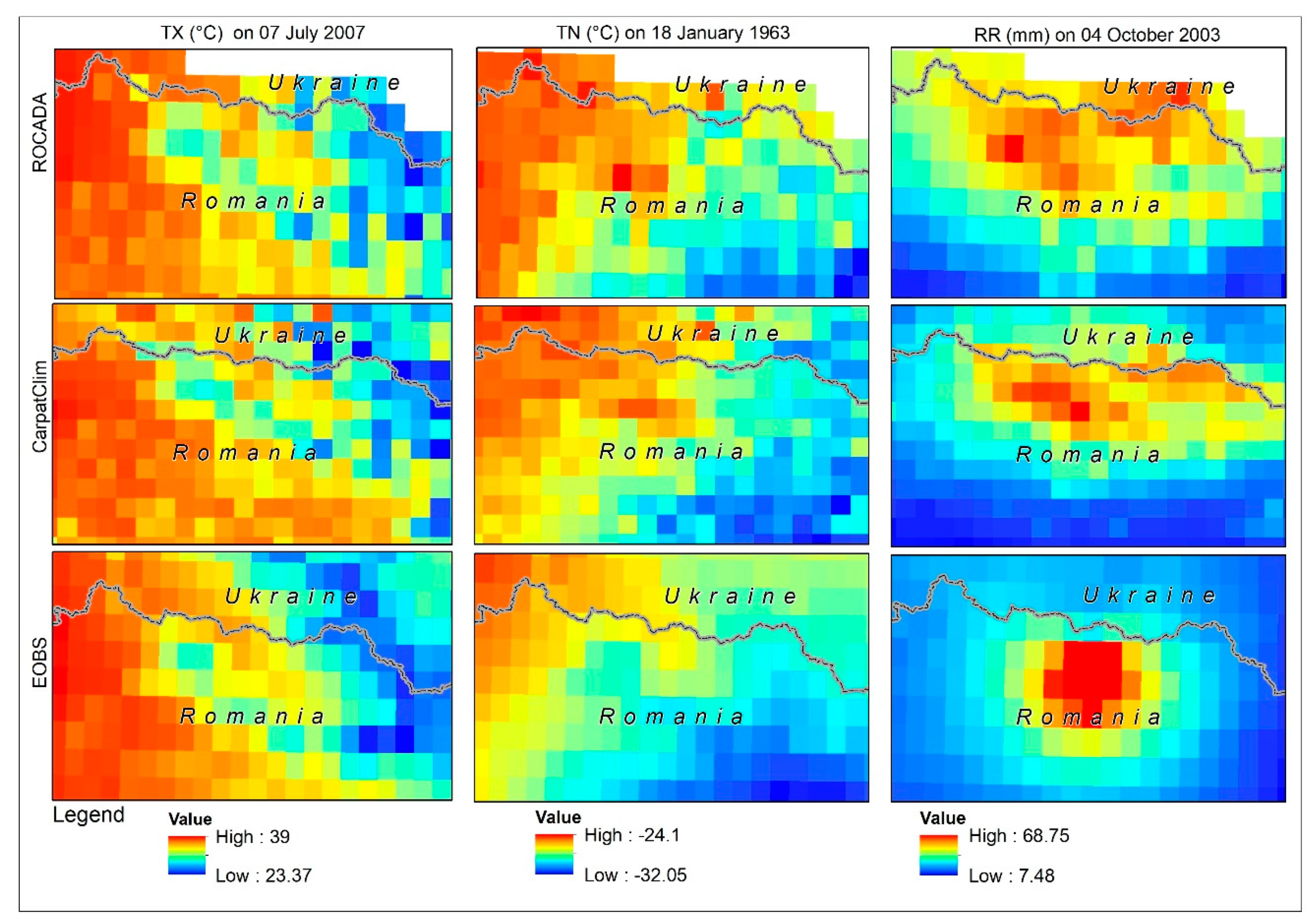
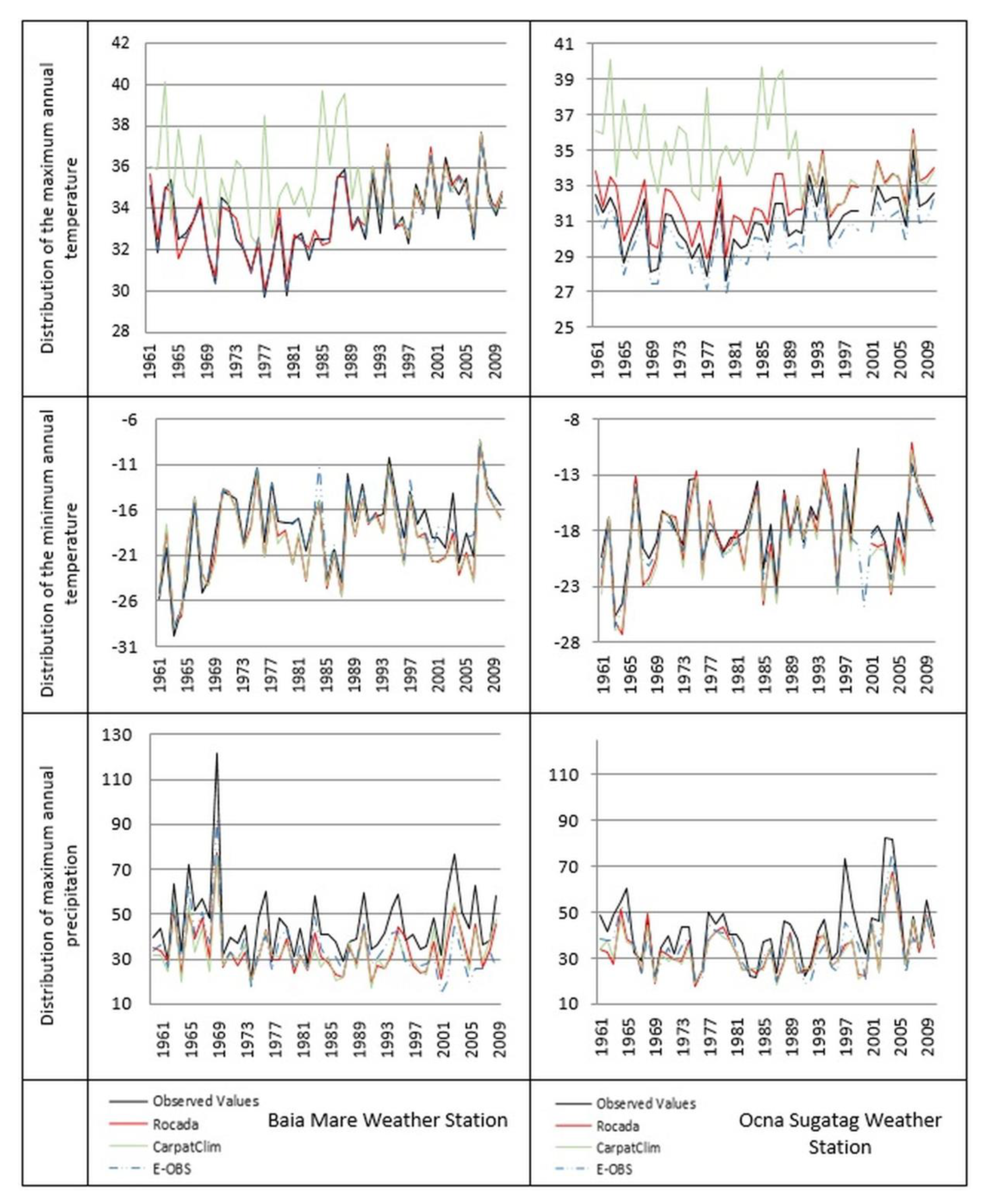
3.2. Analysis of the Historical Extreme Temperatures and Precipitation

The first analysis was performed considering the historical TX and TN values, as well as the highest daily amount of precipitation recorded at the Ocna Șugatag weather station. For the spatial distribution of TX, some anomalies can be observed within the ROCADA and CARPATCLIM gridded datasets (Figure 3). Large temperature differences were detected from one cell to another. Since it is not usual to have such steep differences, we suppose that the methodology of data interpolation could explain this, because the ROCADA and CARPATCLIM datasets used the same method for data homogenization (MASH) and interpolation (MISH) [24,26,27,28], and both datasets have the same distribution anomalies, therefore, it can be assumed that the problem lies in the procedure (method) used for spatial interpolation.

The MASH method broadly assumes that breakpoints and possible changes can be detected and adjusted by mutual comparisons in climate data series. It is based on a series of tests and statistical analyses, described in detail by Szentimrey [24,26,28]. The MISH interpolation method employs homogenized data series (checked by using the MASH method). On the basis of these homogeneous time series, MISH calculates the optimal interpolation parameters depending on the climatic parameter. Therefore, during the data homogenization and interpolation processes, the most important phase is the homogenization procedure along with the number of evaluated climatic parameters and the length of the time series [23,25].

Unlike the ROCADA and CARPATCLIM gridded datasets, to obtain the E-OBS daily gridded dataset, the ordinary Kriging interpolation method was applied [22], which better captured the influence of topography on the analysed climatic parameters.

The E-OBS datasets show a much more accurate spatial distribution for the temperature parameters. However, as compared with extreme temperature series, the precipitation in E-OBS has a different spatial distribution induced, most likely by the much lower density of rainfall stations used in the construction of the gridded dataset (Figure 3).

3.3. Descriptive Statistics

In this section, the values derived from all gridded datasets for both locations were compared with the observation values through descriptive statistics. The entire data series for each variable were employed to derive the descriptive statistics features (

Table 2. Descriptive statistics for the Baia Mare Meteorological Station.

Statistics	TX (°C)				TN (°C)				RR (mm)
	Observation	Rocada	Carpat Clim	E-OBS	Observation	Rocada	Carpat Clim	E-OBS	Observation	Rocada	Carpat Clim	E-OBS
Mean	15.16	15.16	16.13	15.12	5.32	4.69	4.72	5.17	2.47	2.09	2.13	2.12
Standard Error	0.075	0.076	0.078	0.074	0.059	0.060	0.060	0.059	0.04	0.032	0.032	0.034
Median	16.2	16.3	17.48	16.17	6.1	5.47	5.53	5.95	0	0.15	0.14	0
Mode	24	26.33	24.68	23.72	10	0.57	10.64	10.06	0	0	0	0
Standard Deviation	10.08	10.24	10.48	10.03	8.03	8.07	8.12	7.94	5.70	4.31	4.37	4.54
Sample Variance	101.63	104.88	109.75	100.60	64.42	65.12	65.94	63.06	32.43	18.61	19.13	20.64
Kurtosis	−0.98	−1.01	−1.07	−0.99	−0.14	−0.04	−0.07	−0.16	30.99	23.12	22.46	25.80
Skewness	−0.22	−0.23	−0.23	−0.22	−0.52	−0.55	−0.56	−0.52	4.30	3.83	3.79	3.85
Range	53.7	54.53	53.59	53.25	54.8	50.18	50.1	53.29	121.4	77.25	76.09	92.7
Minimum	−16.1	−16.81	−13.48	−16.04	−29.9	−28.59	−28.68	−29.01	0	0	0	0
Maximum	37.6	37.72	40.11	37.21	24.9	21.59	21.42	24.28	121.4	77.25	76.09	92.7
Confidence level (95%)	0.146	0.149	0.152	0.145	0.116	0.117	0.118	0.115	0.083	0.063	0.064	0.066

and

Table 3. Descriptive statistics for the Ocna Șugatag Meteorological Station.

Statistics	TX (°C)				TN (°C)				RR (mm)
	Obser-vation	Rocada	Carpat Clim	E-OBS	Obser-vation	Rocada	Carpat Clim	E-OBS	Obser-vation	Rocada	Carpat Clim	E-OBS
Mean	13.20	14.24	15.70	12.51	3.80	4.31	4.05	3.25	2.05	2.02	2.11	2.07
Standard Error	0.072	0.073	0.079	0.072	0.059	0.061	0.061	0.058	0.036	0.032	0.032	0.033
Median	14.2	15.24	16.97	13.50	4.6	5.08	4.89	4.04	0	0.15	0.190	0
Mode	21	24.99	25.43	21.49	10	6.87	10.92	-0.51	0	0	0	0
Standard Deviation	9.53	9.66	10.44	9.46	7.78	8.05	8.07	7.75	4.87	4.24	4.32	4.39
Sample Variance	90.86	93.40	109.07	89.58	60.52	64.72	65.17	60.11	23.72	17.94	18.63	19.28
Kurtosis	−0.972	−1.006	−1.070	−0.981	−0.387	−0.254	−0.238	−0.360	33.635	24.102	21.729	24.166
Skewness	−0.214	−0.194	−0.225	−0.204	−0.479	−0.511	−0.534	−0.483	4.656	4.005	3.837	3.894
Range	50.6	51.69	53.59	50.41	46.6	47.78	47.06	45.98	82.2	67.74	65.8	76.5
Minimum	−15.6	−15.5	−13.48	−16.25	−25.7	−27.24	−26.93	−26.65	0	0	0	0
Maximum	35.0	36.2	40.1	34.2	20.9	20.5	20.1	19.3	82.2	67.7	65.8	76.5
Confidence level (95%)	0.142	0.144	0.155	0.141	0.116	0.120	0.120	0.114	0.071	0.062	0.063	0.064

). The comparison does not reveal a suggestive indication of the optimal dataset to be used for further analysis; the mean values are, in general, closer to the observed values in the ROCADA gridded dataset, while statistical indices describing the shape of the frequency distribution revealed the E-OBS gridded dataset as providing the closest values to the observations (Table 2 and Table 3).

3.4. Correlation and Determination Analysis of Datasets

Following the methodology described, we performed a specific analysis for all datasets. A very good correlation (higher than 0.95) was obtained for all databases. Pearson’s correlation coefficient indicates different situations for the two meteorological stations. The comparison between the three gridded datasets and the observation values at the Baia Mare meteorological station revealed the best results for ROCADA dataset, while comparing them with the values observed at the Ocna Șugatag meteorological station, the higher correlation coefficient was obtained for the E-OBS dataset (

Table 4. Pearson’s correlation coefficient between gridded and observation data series for TX, TN, and RR (1961–2010).

Variable	Gridded Dataset	MS Baia Mare	MS Ocna Șugatag
TX	ROCADA	0.998	0.997
	CARPATCLIM	0.949	0.997
	E-OBS	0.996	0.999
TN	ROCADA	0.995	0.992
	CARPATCLIM	0.994	0.994
	E-OBS	0.989	0.998
RR	ROCADA	0.954	0.888
	CARPATCLIM	0.952	0.892
	E-OBS	0.913	0.925

).

The highest values were obtained for TN (0.989–0.998) and the lowest for RR (0.888–0.954). Due to the high spatial variability of precipitation, especially in the complex topography regions, one can assume that the correlation for RR is also acceptable (Table 4).

In terms of the coefficient of determination (R-squared), the results are slightly different for the two locations. Thus, for the Baia Mare weather station, the most accurate results for all parameters were obtained for the ROCADA datasets, while for the Ocna Șugatag weather station, the best fit for extreme temperatures was provided by the E-OBS datasets, and for RR by the ROCADA output series.

As in the case of Pearson’s correlation coefficient, it was more difficult to capture precipitation in the models due to a greater spatial variability, nevertheless, when all datasets were considered, quite good values were returned, especially for the ROCADA gridded dataset.

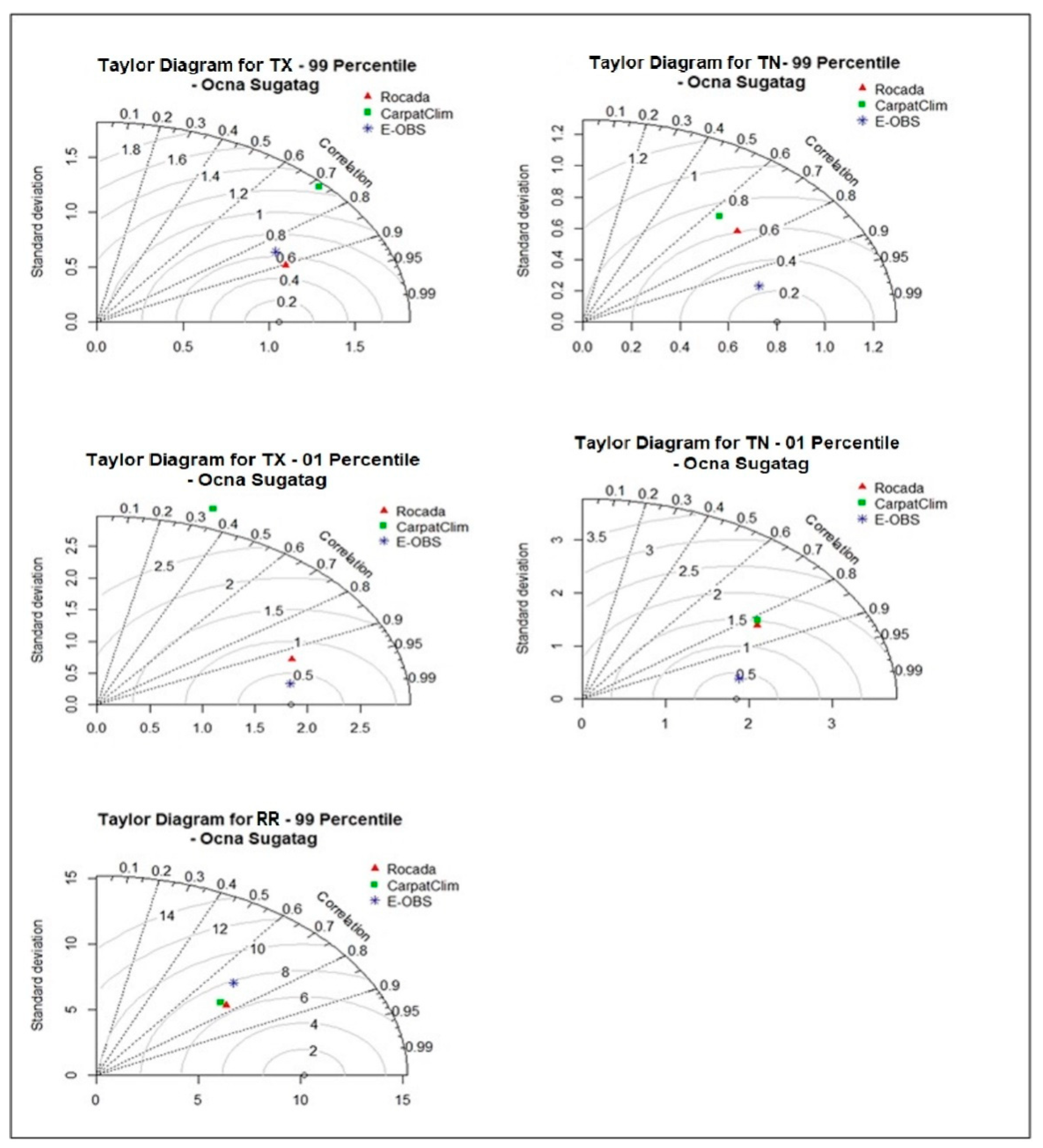
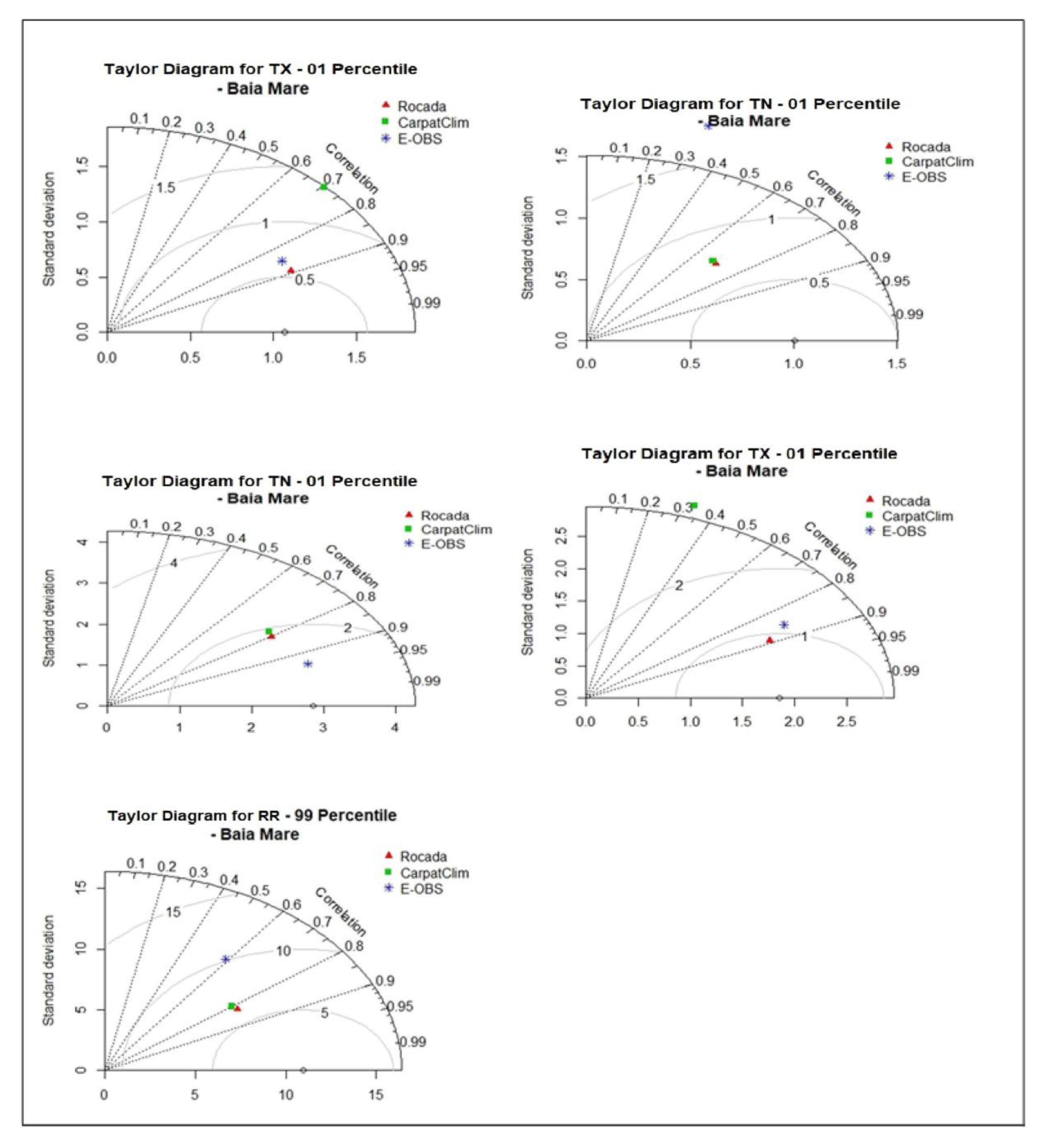
3.5. Taylor Diagrams-Based Analysis

The extreme values of the considered datasets, historical values, and percentile-derived values were further analysed by using Taylor diagrams.

The results are quite different compared to those obtained when full strings were considered. For the extreme percentile values, in the case of TX and TN, the best fit was indicated by the E-OBS database for the Ocna Șugatag weather station (Figure 4), whereas for the Baia Mare weather station, the relationship between the ROCADA and the observed values pairs was found to be the closest for TX and RR (Figure 5).

Using Taylor charts for historical extreme values allowed us to identify the position of gridded data as compared with the reference data. For the 99th percentile (for maximum values), the ROCADA database is generally in a better (closer) position, and for the 1st percentile (for minimum values) the data from E-OBS are more accurate. This was surprising, because to obtain the E-OBS gridded dataset, a lower density of weather stations was used than in the case of the ROCADA and CARPATCLIM databases. It was expected that the ROCADA database, which was developed based on the highest density of weather stations, would better capture the extreme values.

3.6. Linear Regression for the 1st and 99th Percentiles

By employing the linear regression method for the 1st and 99th percentiles series, a similar data layout was obtained as compared with the observation values.

Considering the extreme maximum values (the 99th percentile), the results are different for the two selected locations. For the Baia Mare weather station, the ROCADA database returned the best values for all datasets (

Table 5. Pearson’s correlation coefficient between gridded and observation data series for the 99th percentile values for TX, TN, and RR (1961–2010).

Variable	Gridded Dataset	MS Baia Mare	MS Ocna Șugatag
TX	ROCADA	0.7983 *	0.8895
	CARPATCLIM	0.4994	0.2806
	E-OBS	0.7267	0.9542
TN	ROCADA	0.4981	0.5445
	CARPATCLIM	0.4667	0.4097
	E-OBS	0.1018	0.9073
RR	ROCADA	0.6779	0.5855
	CARPATCLIM	0.6374	0.5447
	E-OBS	0.3458	0.475

* Values in bold are the closest to the observation values.

), whereas, for the Ocna Șugatag weather station, the E-OBS datasets had a better determination coefficient both for the TX and TN series, whilst the ROCADA dataset was the best for RR. In the case of RR, the larger scattering of the points may be induced by the frequent values of 0.0 mm given by the E-OBS dataset when precipitation was actually recorded at the Ocna Șugatag meteorological station for the same days. This could be a consequence of the lower spatial coverage with direct observation stations available for E-OBS interpolation as compared with the much higher density of measurement sites used by the ROCADA database, which returned the best results. The less convenient results were generated by the CARPATCLIM database in terms of extreme temperatures and by the E-OBS database for precipitation (Table 5).

Moreover, the historical minimum values of precipitation are closer in the case of the observed values – E-OBS relation, compared to the other analysed gridded datasets, even though the coefficient of determination value is quite low. As explained above, this low value might be due to the spatial variability of this parameter and to the lower density of stations included in the interpolation to get this dataset.

For the 1st percentile, a better coefficient of determination in relation to the observed values was obtained for E-OBS, both in the case of TX and TN at Ocna Șugatag weather station and for TN at the Baia Mare weather station, while for TX datasets at the Baia Mare weather station, the highest coefficient was obtained between ROCADA dataset and observation data (

Table 6. Pearson’s correlation coefficient between gridded and observation data series for the 1st percentile of the extreme temperature datasets (1961–2010).

Variable	Gridded Dataset	MS Baia Mare	MS Ocna Șugatag
TX	ROCADA	0.7958 *	0.8677
	CARPATCLIM	0.1096	0.1132
	E-OBS	0.7367	0.9678
TN	ROCADA	0.6423	0.6951
	CARPATCLIM	0.6035	0.6676
	E-OBS	0.8784	0.9585

* Values in bold are the closest to the observation values.

). As the 1st percentile for RR is equal to 0 for all datasets considered, we did not calculate the correlation coefficient.

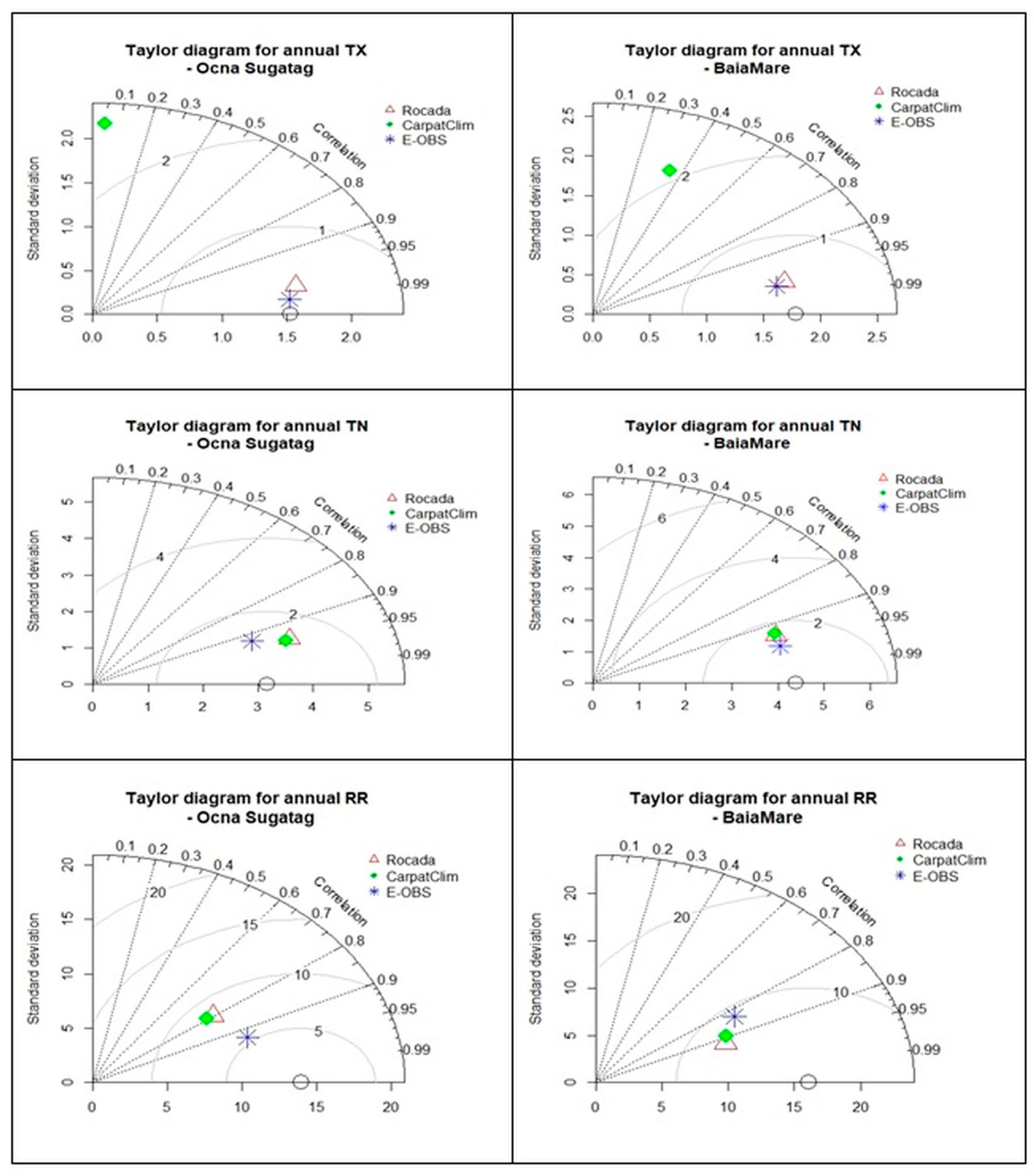
3.7. Analysis of the Extreme Annual Values

The highest and the lowest annual values for each year parameter (TX, TN, and RR) of the considered period were extracted, resulting in 50 values for each dataset. A comparative analysis for the new datasets was performed to identify the best fit between the observation and the derived gridded datasets.

In general, the E-OBS database returned the best results. However, larger differences could be identified, especially after 2000 (Figure 6). The same result was confirmed when using Taylor diagrams (Figure 7).

3.8. Analysis of the Annual Seasonal Values

The extreme seasons’ series were analysed by using three methods: K-S method, Taylor diagrams, and MK trend detection test combined with Sen’s slope for trend magnitude.

3.8.1. Kolmogorov-Smirnov Test (K-S) Distribution Analysis

When analysing the winter TX, TN, and RR datasets by employing the K-S method, the results indicated a cumulative distribution closer to the observation series for the E-OBS gridded dataset in almost all cases (except for TN at Ocna Șugatag weather station). However, the ROCADA output revealed quite small differences compared to the observation time series (

Table 7. The Kolmogorov–Smirnov test (K-S) absolute maximum distribution (D) between the gridded datasets and the observation values for the extreme seasons at the Baia Mare and Ocna Șugatag meteorological stations (1961–2010).

Weather Station	Database	Winter Season			Summer Season
		TX	TN	RR	TX	TN	RR
Baia Mare	ROCADA	0.20 *	0.22	0.42	0.12	0.10	0.20
	CARPATCLIM	0.22	0.20	0.4	0.36	0.10	0.24
	E-OBS	0.20	0.08	0.32	0.10	0.12	0.20
Ocna Șugatag	ROCADA	0.32	0.12	0.54	0.56	0.14	0.22
	CARPATCLIM	0.42	0.18	0.52	0.58	0.16	0.18
	E-OBS	0.26	0.20	0.20	0.34	0.22	0.12

* Values in bold are the closest to the observation values.

).

For summer, the analysis of the same parameters showed a slightly different situation compared to winter: for the TX and TN, the ROCADA gridded dataset presents the lowest values of D, while for the RR series the E-OBS gridded dataset indicates a distribution closer to the observation-derived values (Table 7).

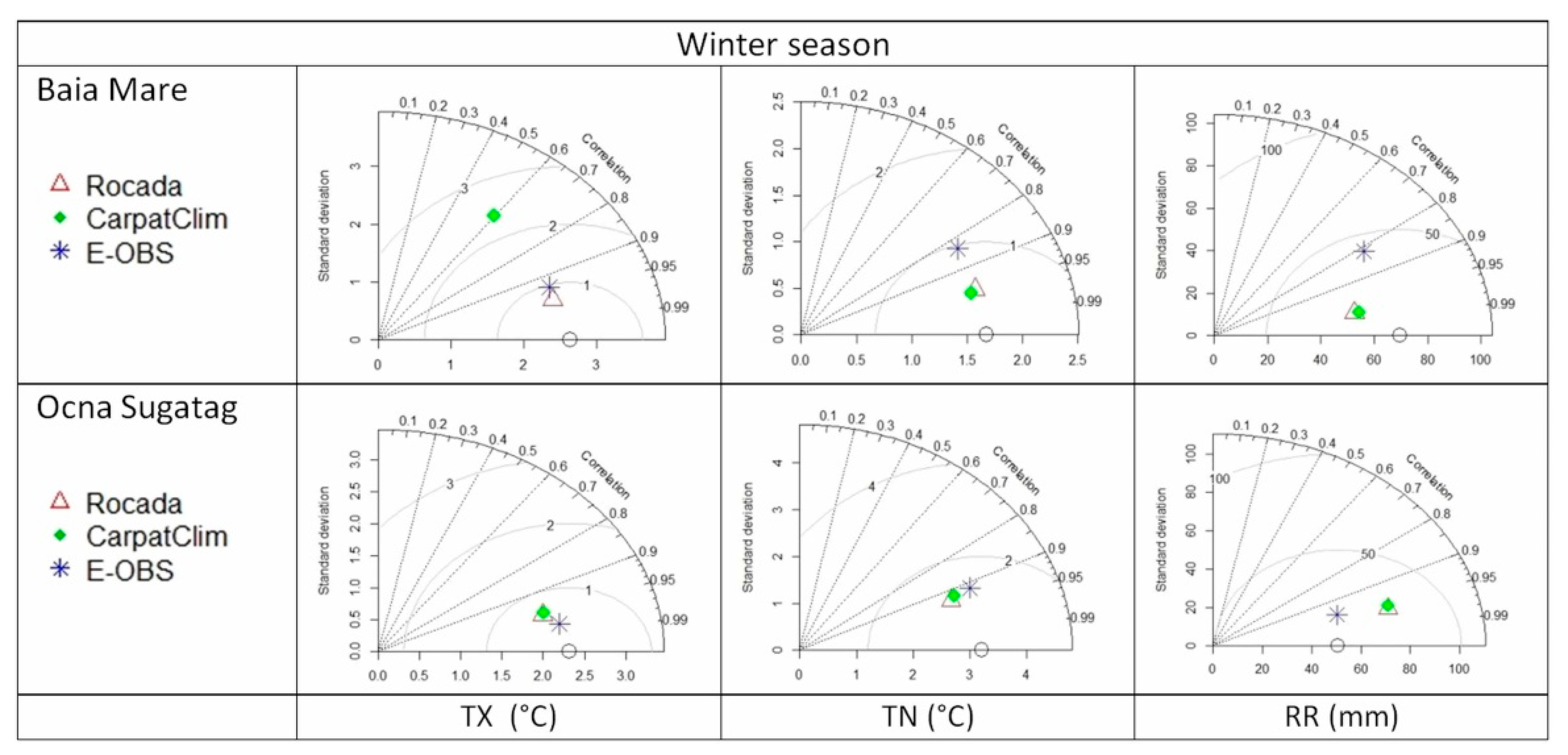
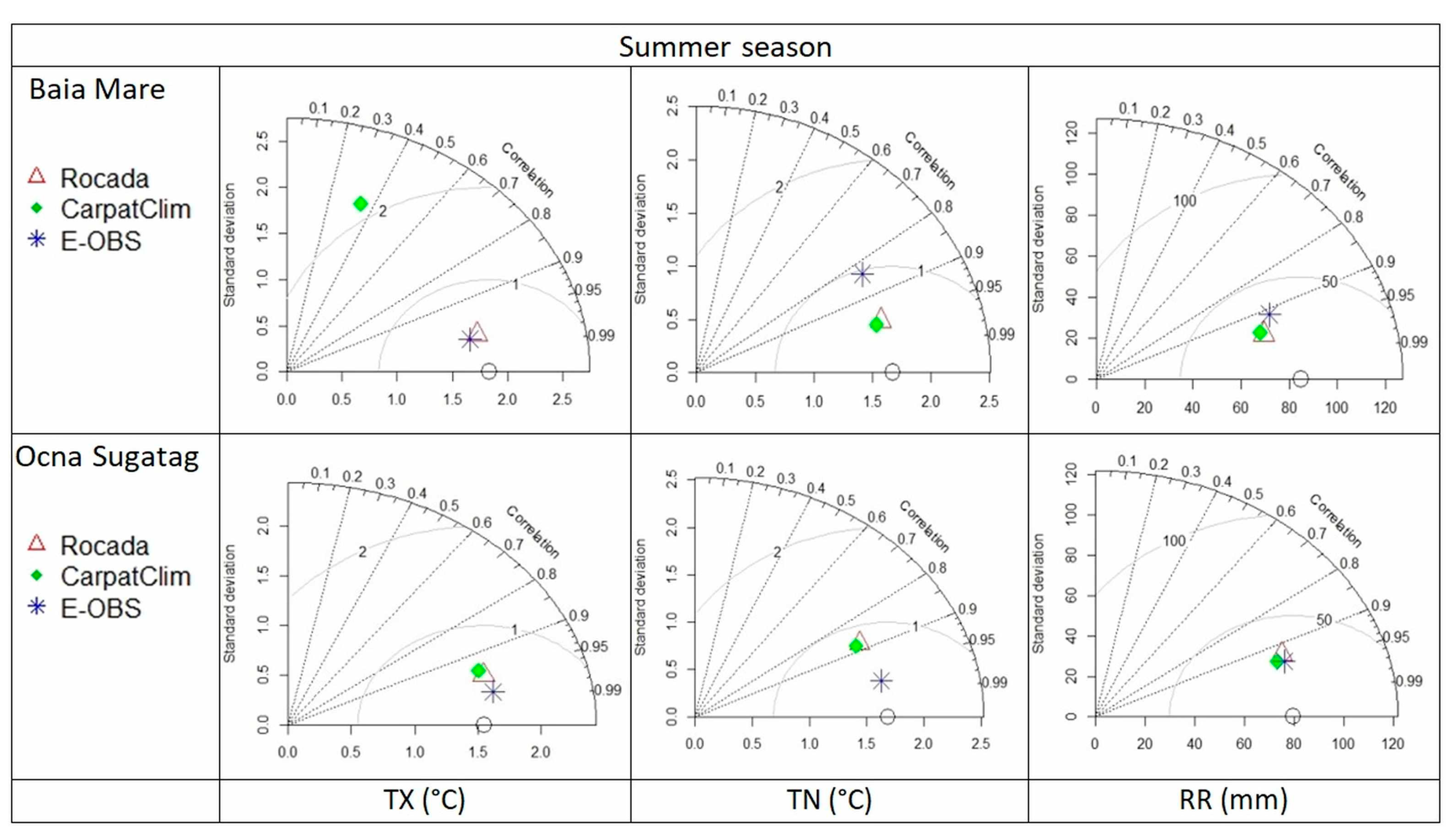
3.8.2. Taylor Diagram Analysis

Taylor diagram-based method was employed for seasonal datasets, too. The analysis revealed a slightly more complicated situation compared to that obtained for the complete datasets: the values of statistical indicators derived from ROCADA datasets, both for winter (Figure 8) and summer (Figure 9) were found to have the best correlation with the statistical indicators of the observation dataset for the Baia Mare weather station and those derived from E-OBS database for the Ocna Șugatag weather station.

3.8.3. Trend Detection

The third approach for seasonal data series consisted in trend detection. The results of the MK test for all analysed datasets for the extreme seasons are presented in

Table 8. Sen’s slope for the summer datasets over the period 1961–2010 at the Baia Mare and Ocna Șugatag weather stations.

Weather Station	Baia Mare				Ocna Șugatag
Time Series	Observations	ROCADA	CarpatClim	E-OBS	Observations	ROCADA	Carpat Clim	E-OBS
TX(°C/year)	0.052 *	0.058	−0.015	0.049	0.050	0.055	0.054	0.048
TN(°C/year)	0.037	0.035	0.030	0.035	0.036	0.030	0.030	0.034
RR(mm/year)	0.470	0.202	0.173	−0.540	0.535	0.385	0.305	−0.248

* Values in bold are statistically significant at α = 0.05.

and

Table 9. Sen’s slope for the winter datasets over the period 1961–2010 at the Baia Mare and Ocna Șugatag weather stations.

Weather Station	Baia Mare				Ocna Șugatag
Time Series	Observations	ROCADA	CarpatClim	E-OBS	Observations	ROCADA	Carpat Clim	E-OBS
TX(°C/year)	0.067 *	0.064	−0.033	0.033	0.056	0.048	0.052	0.048
TN(°C/year)	0.100	0.049	0.050	0.082	0.065	0.047	0.053	0.059
RR(mm/year)	0.733	0.339	0.452	−1.409	−0.007	0.550	0.430	−0.692

* Values in bold are statistically significant at α = 0.05.

. For summer, in terms of slope, the best results for temperature series were returned by E-OBS datasets, while for precipitation ROCADA series indicated the closest slope values to those obtained for observation series. Considering the statistical significance, ROCADA and E-OBS indicated similar results for temperature for the Baia Mare weather station and ROCADA and CarpatClim for the Ocna Șugatag weather station; for precipitation, none of the series was found statistically significant (Table 8).

The winter series indicated the best fit for each parameter with a different database, i.e., for TX with ROCADA and CarpatClim, for TN with E-OBS, and for RR with CarpatClim. In some cases, the trends indicated by CarpatClim or E-OBS are opposite to those detected in the observation-derived series, yet, not statistically significant. Although for TX and TN at the Baia Mare weather station a statistically significant increase was found, none of the grid-derived series indicated a significant change. Moreover, CarpatClim for TX indicated a decreasing trend (Table 9).

4. Conclusions

Gridded datasets are an important source of data for spatial analysis as they offer the possibility to use them as climatic input parameters for different hydrological or agrometeorological models. The main conclusion of the present study is the recommendation of using gridded datasets available for complex topography regions with caution, especially when aiming at illustrating extreme phenomena. Since, sometimes, differences among different gridded datasets are quite significant, the choice of using one or another for further research should be based on prior checking of their consistency with observational data, which is almost a prerequisite to ensure their suitability.

In general, the ROCADA dataset indicated the best fit with the raw observation values across all climatic parameters considered; most likely, a consequence of the highest density of meteorological stations providing observational data employed for developing the gridded data. The programs used to homogenize the data series compared all data strings according to the location of meteorological stations and complemented the lack of data by advanced statistical methods, thus, easing further analysis for researchers.

The CARPATCLIM datasets had the lowest correlation coefficient values between all analysed datasets and for all parameters. Although the same homogenization and spatial interpolation methods and software were used as those employed in creating the ROCADA series (MISH and MASH), the point values showed a fairly wide spread, primarily due to the much lower number of weather stations than the one used for the ROCADA dataset, and, secondarily, because of the reduced density of measuring stations used for the analysed area, which could not adequately capture the influence of topography on the climatic parameters.

Although, in the case of long-term series of data, the E-OBS-derived daily gridded datasets show values rather close to those provided by ROCADA, but not better. When the extreme annual and historical values were considered, series provided by E-OBS fit best to those observed. Thus, among all databases considered for this study, the E-OBS best captures the real (observed) values in terms of extreme values. For trend analysis or for studies based on mean values in North-western Romania, the ROCADA dataset is the most appropriate to be employed.

In general, such assessments of datasets are performed for large geographic regions, in which case many samples are considered for testing, validating one or another climate parameter. However, sometimes, such analyses may prove too cumbersome and often inaccessible due to the large volume of data required, or due to the small size of the selected geographical area for such an analysis. The present study aimed to reveal an alternative evaluation procedure of the existing gridded datasets, organized in four steps; researchers could then identify the one dataset which is the closest to the observation datasets from the total available gridded datasets.

The results of this research show the importance of validating gridded datasets before using them in various research activities. The value and importance of gridded datasets in the research activity cannot be questioned, but their analysis is clearly needed depending on the region they are used for. As a future perspective, we aim to develop this evaluation procedure, which should take into account the quality assessment of datasets in other types of topography regions (e.g., plains, depressions, wetlands, high mountain areas,). Moreover, we intend to increase the number of observation stations to extensively test new analysis methods, such as the network analysis method proposed by Wang and Wang [41].

References

1. Dumitrescu, A.; Bîrsan, M.V. ROCADA: A gridded daily climatic dataset over Romania (1961–2013) for nine meteorologi-cal variables. Nat. Hazards 2015, 78, 1045–1063. [Google Scholar] [CrossRef]
2. Gulizia, C.; Camilloni, I.A. Spatio-temporal comparative study of the representation of pre-cipitation over South America derived by three gridded datasets. Int. J. Climatol. 2015, 36, 1549–1559. [Google Scholar] [CrossRef]
3. Haylock, M.R.; Hofstra, N.; Tank, A.M.G.K.; Klok, E.J.; Jones, P.D.; New, M. A European daily high-resolution gridded data set of surface temperature and precipitation for 1950–2006. J. Geophys. Res. Space Phys. 2008, 113, 113. [Google Scholar] [CrossRef] [Green Version]
4. Costa, A.C.; Soares, A. Homogenization of climate data: Review and new perspectives using geostatistics. Math. Geol. 2009, 41, 291–305. [Google Scholar] [CrossRef]
5. Sluiter, R. Interpolation Methods for the Climate Atlas. KNMI. 2012. 71 p. IR 2009-04. Available online: https://www.semanticscholar.org/paper/Interpolation-Methods-for-the-Climate-Atlas-Sluiter/853b4f9af8b27e4b345e3128b7e69036326979a7 (accessed on 29 September 2020).
6. Singh, H.; Najafi, M.R. Evaluation of gridded climate datasets over Canada using univariate and bivariate approaches: Implications for hydrological modelling. J. Hydrol. 2020, 584, 124673. [Google Scholar] [CrossRef]
7. Aieb, A.; Madani, K.; Scarpa, M.; Bonaccorso, B.; Lefsih, K. A new approach for processing climate missing databases applied to daily rainfall data in Soummam watershed, Algeria. Heliyon 2019, 5, e01247. [Google Scholar] [CrossRef] [Green Version]
8. Bartók, B.; Tobin, I.; Vautard, R.; Vrac, M.; Jin, X.; Levavasseur, G.; Denvil, S.; Dubus, L.; Parey, S.; Michelangeli, P.-A.; et al. A climate projection dataset tailored for the European energy sector. Clim. Serv. 2019, 16, 100138. [Google Scholar] [CrossRef]
9. Darand, M.; Khandu, K. Statistical evaluation of gridded precipitation datasets using rain gauge observations over Iran. J. Arid. Environ. 2020, 178, 104172. [Google Scholar] [CrossRef]
10. Ekström, M.; Grose, M.; Heady, C.; Turner, S.; Teng, J. The method of producing climate change datasets impacts the resulting policy guidance and chance of mal-adaptation. Clim. Serv. 2016, 4, 13–29. [Google Scholar] [CrossRef] [Green Version]
11. Faiz, M.A.; Liu, D.; Fu, Q.; Sun, Q.; Li, M.; Baig, F.; Li, T.; Cui, S. How accurate are the performances of gridded precipitation data products over Northeast China? Atmos. Res. 2018, 211, 12–20. [Google Scholar] [CrossRef]
12. Yao, J.; Chen, Y.; Yu, X.; Zhao, Y.; Guan, X.; Yang, L. Evaluation of multiple gridded precipitation datasets for the arid region of northwestern China. Atmos. Res. 2020, 236, 104818. [Google Scholar] [CrossRef]
13. Musie, M.; Sen, S.; Srivastava, P. Comparison and evaluation of gridded precipitation datasets for streamflow simulation in data scarce watersheds of Ethiopia. J. Hydrol. 2019, 579, 124168. [Google Scholar] [CrossRef]
14. Nashwan, M.S.; Shahid, S. Symmetrical uncertainty and random forest for the evaluation of gridded precipitation and temperature data. Atmos. Res. 2019, 230, 104632. [Google Scholar] [CrossRef]
15. Serrano-Notivoli, R.; De Luis, M.; Beguería, S. An R package for daily precipitation climate series reconstruction. Environ. Model. Softw. 2017, 89, 190–195. [Google Scholar] [CrossRef] [Green Version]
16. Nechita, C.; Čufar, K.; Macovei, I.; Popa, I.; Badea, O.N. Testing three climate datasets for dendroclimatological studies of oaks in the South Carpathians. Sci. Total Environ. 2019, 694, 133730. [Google Scholar] [CrossRef]
17. Szentimrey, T.; Bihari, Z. Manual of interpolation software MISHv1.03. In Hungarian Meteorological Service; Hungarian Meteorological Service: Budapest, Hungary, 2014; p. 89. [Google Scholar]
18. Soares, M.B.; Alexander, M.; Dessai, S. Sectoral use of climate information in Europe: A synoptic overview. Clim. Serv. 2018, 9, 5–20. [Google Scholar] [CrossRef]
19. Sfîcă, L.; Stratulat, I.S.; Hrițac, R.; Ichim, P.; Ilie, N. Favorabilitatea climatică a teritoriului României pentru activități turistice de tip balnear în sezonul estival. In Stratulat, IS Coord—Balneoclimatologia în România și Republica Moldova—Istoric și Perspective Europene; Editura Academiei Române: Bucharest, Romania, 2018; Volume 409, pp. 327–347. ISBN 978-973-27-3005-8. [Google Scholar]
20. Sfîcă, L.; Iordache, I.; Voiculescu, M. Solar signal on regional scale: A study of possible solar impact upon Romania’s climate. J. Atmos. Solar-Terr. Phys. 2018, 177, 257–265. [Google Scholar] [CrossRef]
21. Dobri, R.-V.; Sfîcă, L.; Ichim, P.; Harpa, G.-V. The distribution of the monthly 24-hour maximum amount of precipitation in romania according to their synoptic causes. Geogr. Tech. 2017, 12, 62–72. [Google Scholar] [CrossRef] [Green Version]
22. Tank, A.M.G.K.; Wijngaard, J.B.; Können, G.P.; Böhm, R.; Demarée, G.; Gocheva, A.; Mileta, M.; Pashiardis, S.; Hejkrlik, L.; Kern-Hansen, C.; et al. Daily dataset of 20th-century surface air temperature and precipitation series for the European Climate Assessment. Int. J. Clim. 2002, 22, 1441–1453. [Google Scholar] [CrossRef]
23. European Climate Assessment and Datasets. Available online: www.ecad.eu (accessed on 23 March 2020).
24. Climate of the Carpathian Region. Available online: http://www.carpatclim-eu.org (accessed on 15 January 2020).
25. Croitoru, A.E.; Piticar, A.; Sfîcă, L.; Harpa, G.V.; Roșca, C.F.; Tudose, T.; Horvath, C.; Minea, I.; Ciupertea, F.A.; Scripcă, A.S. Extreme Temperature and Precipitation Events in Romania; Editura Academiei Române: Bucharest, Romania, 2018. [Google Scholar]
26. Szalai, S.; Auer, I.; Hiebl, J.; Milkovich, J.; Radim, T.; Stepanek, P.; Zahradnicek, P.; Bihari, Z.; Lakatos, M.; Szentimrey, T.; et al. Climate of the Greater Carpathian Region; Final Technical Report; Publications Office of the European Union: Budapest, Hungary, 2013. [Google Scholar]
27. Szentimrey, T.; Bihari, Z. Manual of interpolation software MISHv1.01. In Hungarian Meteorological Service; Hungarian Meteorological Service: Budapest, Hungary, 2005. [Google Scholar]
28. Szentimrey, T. Manual of homogenization software MASHv3. In Hungarian Meteorological Service; Hungarian Meteorological Service: Budapest, Hungary, 2011. [Google Scholar]
29. Description of MASH and MISH Algorithms. Available online: http://www.carpatclim-eu.org/docs/mashmish/mashmish.pdf (accessed on 15 March 2020).
30. Cornes, R.C.; Van Der Schrier, G.; Besselaar, E.J.M.V.D.; Jones, P.D. An ensemble version of the E-OBS temperature and precipitation data sets. J. Geophys. Res. Atmos. 2018, 123, 9391–9409. [Google Scholar] [CrossRef] [Green Version]
31. Taylor, K.E. Summarizing multiple aspects of model performance in a single diagram. J. Geophys. Res. Atmos. 2001, 106, 7183–7192. [Google Scholar] [CrossRef]
32. Engmann, S.; Cousineau, D. Comparing distributions: The two-sample Anderson–Darling test as an alternative to the Kolmogorov–Smirnov test. J. Appl. Quant. Methods 2011, 6, 1–17. [Google Scholar]
33. Mann, H.B. Non-parametric tests against trend. Econometrica 1945, 13, 245–259. [Google Scholar] [CrossRef]
34. Kendall, M.G. Rank Correlation Methods, 4th ed.; Charles Griffin: London, UK, 1975. [Google Scholar]
35. Gilbert, R.O. Statistical Methods for Environmental Pollution Monitoring; John Wiley & Sons: Hoboken, NJ, USA, 1987. [Google Scholar]
36. Wu, W.; Dessler, A.E.; North, G.R. Analysis of the correlations between atmospheric boundary-layer and free-tropospheric temperatures in the tropics. Geophys. Res. Lett. 2006, 33, L20707. [Google Scholar] [CrossRef]
37. Some’E, B.S.; Ezani, A.; Tabari, H. Spatiotemporal trends and change point of precipitation in Iran. Atmos. Res. 2012, 113, 1–12. [Google Scholar] [CrossRef]
38. Tabari, H.; Nikbakht, J.; Talaee, P.H. Identification of trend in reference evapotranspiration series with serial dependence in Iran. Water Resour. Manag. 2012, 26, 2219–2232. [Google Scholar] [CrossRef]
39. Tabari, H.; Aghajanloo, M.-B. Temporal pattern of aridity index in Iran with considering precipitation and evapotranspiration trends. Int. J. Clim. 2013, 33, 396–409. [Google Scholar] [CrossRef]
40. Salmi, T.; Määttä, A.; Anttila, P.; Ruoho-Airola, T.; Amnell, T. Detecting trends of annual values of atmospheric pollutants by the Mann-Kendall Test and Sen’s solpe estimates the excel template application MAKESENS. Publ. Air Qual. 2002, 7, 31. [Google Scholar]
41. Wang, C.; Wang, Z.-H. A network-based toolkit for evaluation and intercomparison of weather prediction and climate modeling. J. Environ. Manag. 2020, 268, 110709. [Google Scholar] [CrossRef]
Figure 1. Location of the meteorological stations considered.
Atmosphere 12 00361 g001
Figure 2. Spatial domains for the databases used in this study.
Atmosphere 12 00361 g002
Figure 3. Spatial distribution of the historical maximum temperature (TX), minimum temperature (TN), and precipitation (RR) values in the focus region.
Atmosphere 12 00361 g003
Figure 4. Taylor diagram for the 1st and 99th percentiles, the Ocna Șugatag weather station.
Atmosphere 12 00361 g004
Figure 5. Taylor diagram for the 1st and 99th percentiles, the Baia Mare weather station.
Atmosphere 12 00361 g005
Figure 6. Extreme annual TX, TN, and RR values derived from observation and gridded datasets over the period 1961–2010 at the Baia Mare and Ocna Șugatag weather stations.
Atmosphere 12 00361 g006
Figure 7. Taylor diagrams for the extreme annual values (TX, TN, and RR) over the period 1961–2010 at the Ocna Șugatag and Baia Mare weather stations.
Atmosphere 12 00361 g007
Figure 8. Taylor diagrams for winter (TX, TN, and RR) at the Baia Mare and Ocna Șugatag weather stations (1961–2010).
Atmosphere 12 00361 g008
Figure 9. Taylor diagrams for summer (TX, TN, and RR) at the Ocna Șugatag and Baia Mare weather stations (1961–2010).
Atmosphere 12 00361 g009