Article

Documented and Simulated Warm Extremes during the Last 600 Years over Monsoonal China

1
Department of Atmospheric Science, School of Environmental Studies, China University of Geosciences, Wuhan 430074, China
2
Faculty of Geography Science, Beijing Normal University, Beijing 100875, China
3
Norce Research Climate, Uni Research, Bjerknes Center for Climate Research, N-0007 Bergen, Norway
4
Nansen-Zhu International Research Centre, Institute of Atmospheric Physics, Chinese Academy of Sciences, Beijing 100029, China
*
Author to whom correspondence should be addressed.
Atmosphere 2021, 12(3), 362; https://doi.org/10.3390/atmos12030362
Submission received: 3 February 2021 / Revised: 27 February 2021 / Accepted: 5 March 2021 / Published: 9 March 2021
(This article belongs to the Section Climatology)

Abstract

:
In this study, we present an analysis of warm extremes over monsoonal China (21–45° N, 106–124° E) during the last 600 years based on Chinese historical documents and simulations from the Paleoclimate Modelling Intercomparison Project Phase 3 (PMIP3) and the Coupled Model Intercomparison Project Phase 5 (CMIP5). The Chinese historical documents indicate that extreme warm records become more frequent after ~1650 CE in North China and ~1850 CE in the Yangtze River Valley. Our analyses of two threshold extreme temperature indices also illustrate that warm extremes have become more frequent since the 17th century in North China and the mid-19th century in Yangtze River Valley in good agreement with the changes in warm extremes revealed in the historical documents. This agreement suggests potential mechanisms behind the shift of periods, which should be further investigated in the future.

1. Introduction

The last 600 years is a crucial period that links the last millennium together with the recent warming climate. It generally can be divided into two periods, the Little Ice Age (LIA; 1400–1849 CE) and the 20th Century Warming Period (20C WP; 1850–2005 CE). The LIA was first mentioned by Matthes who intended to describe glacial regrowth in the Sierra Nevada, California [1]. Later, this concept was used to describe the latest and extensive occurrence of glacial activities in the late Holocene [2]. Paleoclimate proxies and climate simulations indicated that the global mean surface air temperatures (SAT) during the LIA were about 0.5–1.5 °C colder than the early 1800s [3,4]. However, the onset, duration and temperature changes during the LIA seem to be highly regional-dependent [5,6,7,8]. After the end of the LIA, a warming trend occurred that lasted into the 20C WP [9,10]. Within the 20C WP, the globally averaged surface temperatures over land and ocean showed a linear warming trend of 0.85 °C (according to the Intergovernmental Panel on Climate Change a 90% likelihood of varying between 0.65 °C and 1.06 °C) from 1880 to 2012 CE [11].
During the last 600 years, global and regional climates show remarkable variations as demonstrated in many proxy records as well as historical documents [12,13,14,15,16]. There are prominent cold periods; the middle 15th century, the early 17th and the early 19th century can be found during the LIA [17,18,19]. The global climate during the 20C WP includes a slight cooling (late 19th century) then the early twentieth century warming (ETCW; 1901–1950 CE) [20] and finally the recent warming hiatus (1998–2012 CE) [21,22]. According to previous studies, the increased frequency and severity of climate extremes can be found during the 20C WP [23,24,25].
At multiple timescales, climate changes are influenced by anthropogenic factors, volcano eruptions and the natural variability of the Earth’s system [26], which include solar factors and many climatic oscillations such as the Atlantic Multidecadal Oscillation, Pacific Decadal Oscillation, North Atlantic Oscillation, Arctic Oscillation and others [27]. Among solar factors, solar activities (the magnetic field of the Sun) also influence the climate except for solar irradiance [28,29].
China has long been a densely populated country with progress in civilization from several transitions in dynasties. Many extreme climate events are recorded in Chinese history during this period; for example, the maximum summer temperature in northern China in 1743 CE [30] and the extremely cold temperature in 1816 CE [31]. These events led to changes in socio-economic conditions [32], human health [33], safety [34], survival [35] and ecosystems [36].
Therefore, climate variabilities during the last 600 years attract much interest not only from proxies but also from modelling studies in China. Using the global atmosphere-ocean coupled model ECHO-G, Liu et al. [37] revealed that the simulated low-frequency climate variabilities during the LIA agree well with the reconstructions based on Chinese historical documents [14]. Using the fully coupled three-dimensional model CCSM 2.0.1, Peng et al. [38] pointed out that simulated temperature variabilities remained weaker than the reconstruction [14] in eastern China. The simulations with the UVic Earth System Climate model show that the correlation coefficient between simulated [39] and reconstructed [40] temperatures is 0.5 in eastern China.
However, less attention is paid to understanding warm extremes during the last 600 years because the LIA is a cold period. To further improve the understanding of climate extreme events in monsoonal China (21–45° N, 106–124° E), in this study we compare documented and simulated warm extremes. We firstly use Chinese historical records to identify warm extremes and then evaluate the simulated warm extremes with the models that participated in the Paleoclimate Modelling Intercomparison Project Phase 3 (PMIP3) and the Coupled Model Intercomparison Project Phase 5 (CMIP5).

2. Datasets and Methods

2.1. Datasets

2.1.1. Historical Documents Data

Documented records have unique advantages for the reconstruction of the past climate. They have the characteristics of high spatial and temporal resolution with accurate age control and clear climate meaning [41]. A few comprehensive integrated achievements such as the compilation of documentary records and electronic databases have provided a reference for analyzing the last millennium climate. Numerous studies of climate extremes using historical documents have been done [42,43,44,45].
Two classical books are used in this study, “A Collection Of Meteorological Records For The Past 3000 Years In China” [46] and “Meteorological Disaster Of China” [47]. The first book was written by Deer Zhang in 2004 and served as a chronological record. It is the symbol of the success of Chinese historical climatology. It contains records of local weather or climate conditions and related disaster records from the 13th century BC to 1911 CE. A total of 8228 kinds of relevant records of ancient documents was collected and organized in the process of compiling this book. The second book was written by Kegang Wen in 2005. It records droughts, heatwaves, low temperatures, typhoons and other meteorological disasters taking years as the unit. There are 32 volumes (including comprehensive and local volumes) in this book. We mainly focus on the volumes related to eastern China provinces. The original records of these two works mainly come from the “zai xiang (灾祥)” or “xiang yi (祥异)” part of the local chronicles, which mainly cover the special astronomical phenomena and agrometeorological events that occurred each year.

2.1.2. Climate Model Data

The modelling outputs came from the last millennium (LM) experiments in PMIP3 [48] and the historical experiments in CMIP5 [49] simulated with CCSM4, BCC-CSM1.1, CSIRO-Mk3L-1–2, MPI-ESM-P, MRI-CGCM3 and IPSL-CM5A-LR (Table 1). All models with daily outputs were employed in this study except for MIROC-ESM due to its abnormal warming in the LM experiment [3,50,51]. Only the first run (tagged with r1i1p1 in the Earth System Grid Federation database, ESGF) for each model was used in this study. Basic information of the six models is shown in Table 1 and these data can be downloaded at the website of https://esgf-node.llnl.gov/projects/cmip5/ (accessed on 5 January 2021). Note IPSL-CM5A-LR only provides the daily outputs from 1500 to 2005 CE. Detailed climate forcing and experimental designs are introduced at the PMIP website (https://pmip3.lsce.ipsl.fr/wiki/doku.php/pmip3:design:lm:final/ accessed on 13 December 2020) and the CMIP website (pcmdi.llnl.gov/mips/cmip5/ accessed on 18 December 2020).
Although there is still bias between observations and simulations, the performance of these six models had a modest improvement compared with CMIP3 in simulating the factors that modulate temperature variations such as the EI Niño Southern Oscillation [52], Atlantic Multidecadal Oscillation and Pacific Decadal Oscillation [53].

2.1.3. Observation Data

To validate the simulated warm extremes, we used the modern observational dataset CN05.1 (Figure 1). CN05.1 is a high-quality dataset of gridded Tmax and Tmin established from 2416 stations over China by the National Climate Center of the China Meteorological Administration [54,55].
All of the simulations and observations were interpolated to a relatively median horizontal resolution of 2° × 2°.

2.2. Methods

2.2.1. Warm Records in Chinese Historical Documents

We used a semantic judgment method to select extreme warm records in the historical documents. These keywords can be classified into three categories. The first is the direct descriptions of heat. Many Chinese words, for example, kushu (酷暑), shengshu (盛暑), shenshu (甚暑), yan (炎), re (热), xunzhuo (熏灼) and yv (燠), indicate that it was very hot. The second is the description of the sun and winds in hot scenarios. For example, sunshine like fire (ri ru hu, 日如火), the sun is shining and it is very dry (kang yang, 亢阳), hot winds like fire (yan feng ru huo, 炎风如火) and hot air burns skins (jiao qi chu ren, 焦气触人). The third is the description of the biological responses of humans or animals, for example, people die of heatstroke (ren ye si, 人暍死), female farmers die of heatstroke (tian fu ye si, 田妇暍死), seedling of cereal crops wither (he miao jin ku, 禾苗尽枯) due to hot and dry conditions and fish die in drying rivers (he yv si, 河鱼死).
In principle, the keywords in the first category were necessary to identify warm extremes. However, when the keywords from the first category were missing, the co-occurring of keywords from the second and the third category were considered as auxiliary discriminant criteria.

2.2.2. Extreme Temperature Indices

Three indices, recommended by the Expert Team on Climate Change Detection and Indices (ETCCDI), were used to represent simulated warm extremes in this study [61,62,63,64]. They were the two threshold indices TX90p and TN90p and the duration index WSDI. TX90p (TN90p) was calculated as the percentage of days when Tmax (Tmin) was greater than a 90th percentile, representing the proportion of warm extremes. WSDI, which represented the duration of warm extremes, was calculated as an annual count of days with at least six consecutive days when Tmax was greater than a 90th percentile. The definitions of these three indices can be found at the ETCCDI website (http://etccdi.pacificclimate.org/list_27_indices.shtml/ accessed on 9 January 2021). For each simulation and the CN05.1 observations, the values between 1961 and 1990 CE were used as the reference to get the 90th percentile for these three indices.

2.2.3. Model Validation

Taylor diagrams [65] were employed to validate the ability of models to simulate spatial variation and interannual variability of the extreme temperature indices. Taylor diagrams need three parameters, the correlation coefficient (CC), the root-mean-square (RMS) difference between the two time series and the ratio of the standard deviations (RSD) of the two patterns. In the Taylor diagrams of spatial variations, we calculated the three parameters based on the mean field of three indices (Figures S1 and S2) in monsoonal China during 1961–2005 CE. In the Taylor diagrams of interannual variability, we calculated the three parameters based on the time series (Figures S3–S5) of three indices averaged (area-weighted) in monsoonal China during 1961–2005 CE.

2.2.4. Analyses of Simulated Warm Extremes

We used wavelet analyses to illustrate periods in the indices. The wavelet transform is a mathematical tool to supply time-frequency representations of an analyzed signal in a time domain [66]. In comparison with classical spectral analyses, wavelet analyses can quantify temporal variabilities on different scales but do not need a stationary series [67]. Thus, the method can analyze irregularly distributed events and time series that contain non-stationary power at different frequencies [68]. The mother function of wavelet analyses is the Morlet wavelet, which provides a balance between time and frequency localization and includes the exponential function modulated by a Gaussian wavelet [69].
We also employed trend analyses to show the trend of extreme temperature indices. As most of the extreme temperature indices did not follow a Gaussian distribution [70], the linear least squares estimation, though popular, could not be used in the trend analyses of extreme temperature indices. Instead, we used the non-parametric Theil–Sen method [71] to calculate the trend. Meanwhile, we used the Mann–Kendall test [72,73] to examine if the trend was statistically significant at the 95% confidence level.

3. Results

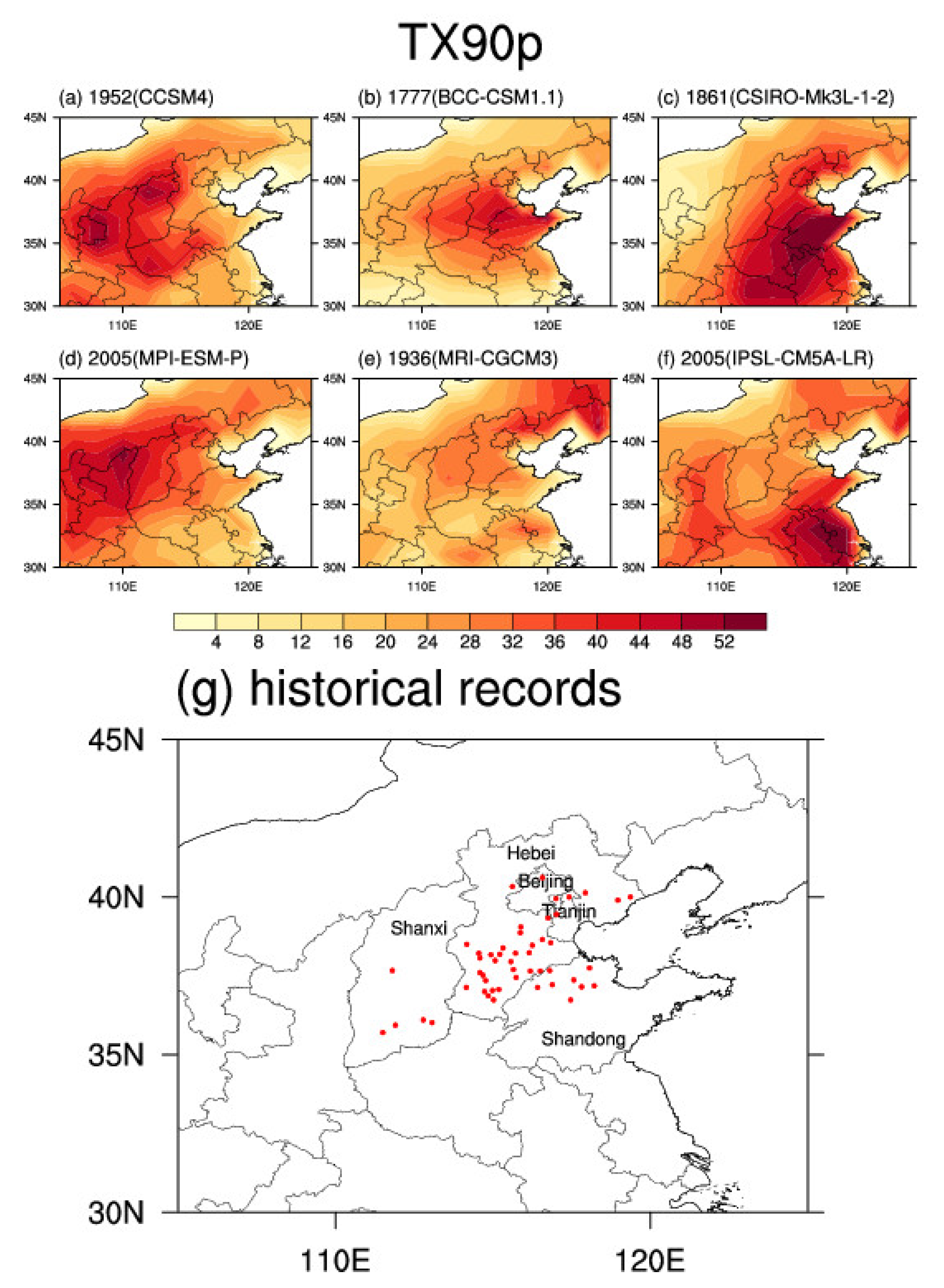
3.1. Warm Extremes in Historical Documents

Figure 2d shows the frequency of documented extreme warm records within a five decadal interval. For example, 0.3 means three years in the decadal interval. There were 151 records of warm extremes over monsoonal China during the last 600 years. Among them, 128 records appeared in NC and 22 happened in YRV while only one was from SC (Table 2). We found that warm records of monsoonal China became more frequent after ~1850 CE as shown in Figure 2d. A similar feature can be found in Figure 2a–c. There was a significant increasing trend of the simulated Tmax, Tmin and reconstructed annual mean temperatures since 1850 CE. Previous studies have proved warm extremes became more frequent under the background of global warming [25].
During the LIA, documented warm extremes mainly concentrated on 1710–1760 CE whereas the frequency of warm extremes was low during 1440–1480 CE (Figure 2d, black bars). Previous studies based on historical documents have found that the middle of the 15th century was the cold period [15] while 1710–1760 CE was the relatively warm period [74]. Note that the two characteristic periods can be found in the simulated results (Figure 2a,b) and reconstructions by Hao et al. [75] (Figure 2c).
For three regions of monsoonal China, the frequency of warm extremes was regionally-dependent. The statistics of records per decade showed that extreme warm events became more frequent after ~1650 CE in NC than before (red bars). In YRV, a change in frequency occurred after 1850 CE (blue bars). However, there was only one record in SC (green bar).

3.2. Warm Extremes in Simulations

3.2.1. Changes of Warm Extremes from the LIA to 20C WP

Figure 3 shows the histograms of simulated summer mean Tmax and Tmin temperatures. Almost all of the models produced right-side shifts of post-1850 temperature distributions relative to pre-1850, indicating a remarkable recent climate warming in monsoonal China. Compared with the 90th percentile threshold in the reference period (1961–1990 CE), the pre-1850 temperature distributions often showed fewer areas above the threshold while the post-1850 temperature distributions showed more areas above the threshold, suggesting a higher frequency of warm extremes during the 20th century [62,64,76]. However, MRI-CGCM3 behaved differently when compared with the other five models. The right-side shift of the post-1850 Tmax relative to the pre-1850 was smaller than the other five models.

3.2.2. Validation of Indices

The model validation (Figure 4a) demonstrated that models had better abilities in simulating the spatial variation in the TX90p and TN90p indices than in the WSDI index. In the Taylor diagram, the simulated TX90p and TN90p indices had spatial correlation coefficients (dotted radial lines) 0.95–0.99 to the CN05.1 observations (during 1961–2005 CE) while the spatial correlation coefficients for the simulated WSDI index were lower, ranging between 0.7–0.95. Almost half of the models used here simulated smaller variances (black dotted circular lines) of the spatial distributions of these indices (with a ratio between 0.75 and 1) than the CN05.1 observation whereas other models reproduced larger variances (ranging between 1 and 1.5). TX90p and TN90p showed smaller RMS differences (less than 0.5) while the RMS differences of WDSI ranged between 0.5 and 1.
In the case of the interannual variability (Figure 4b), TN90p showed relatively higher temporal correlation coefficients (ranging between 0.7–0.35) than the CN05.1 observation, relative to TX90p. However, the relatively high correlation could be due to global warming and it needs further study. Although most models reproduced similar temporal variances (varying between 1.0–1.25) to the CN05.1 observation, the RMS differences were large (larger than 0.5) and showed a remarkable spread. CCSM4, BCC-CSM1.1 and IPSL-CM5A-LR provided relatively better simulations in the interannual variability of TN90p.
Therefore, these six models had a better performance in simulating the threshold indices (TX90p and TN90p). In the analyses below, we only diagnosed the two threshold indices.

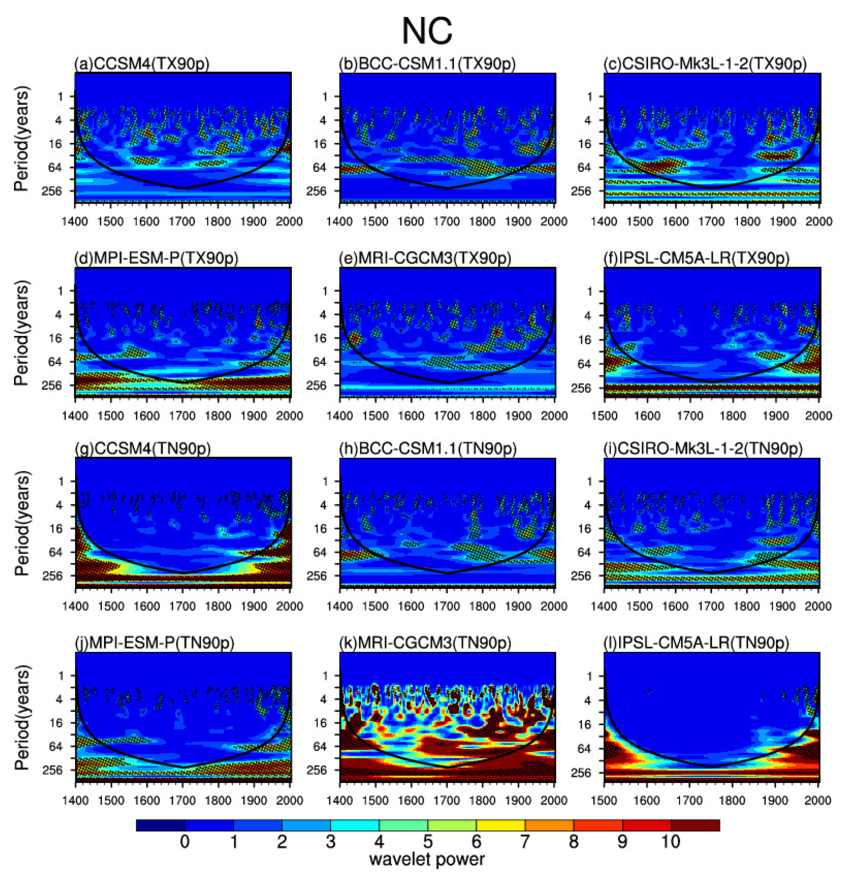
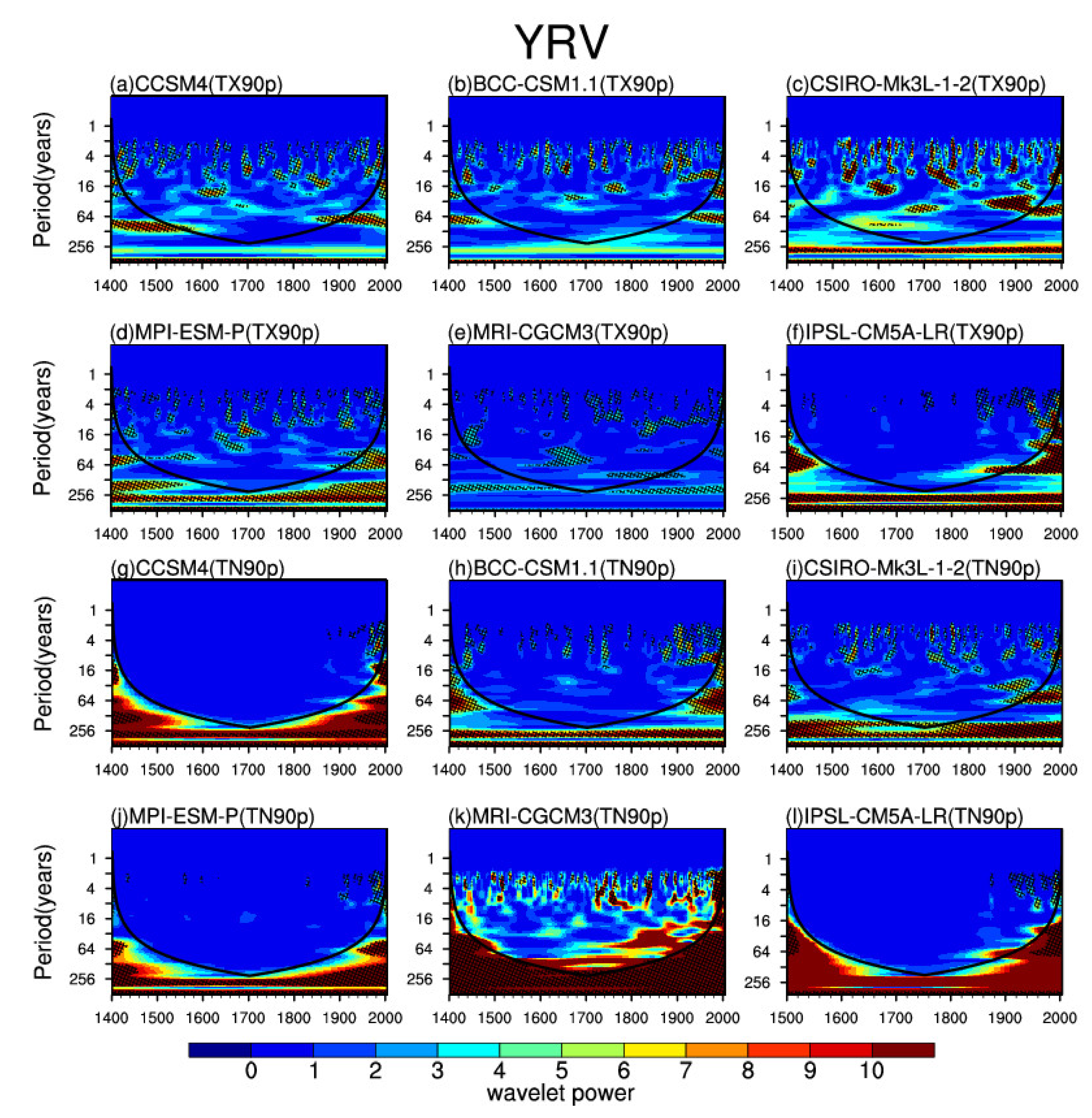
3.2.3. Changes of Indices during 1400–2005 CE

The wavelet analyses of TN90p and TX90p suggested a shift in warm extremes since the 17th century in NC (as indicated by a weakened ~60-year period in TN90p around 1600 CE simulated with CSIRO-Mk3L-1–2 and MPI-ESM-P in Figure 5i,j), a strengthened 32–128-year period in TN90p from around 1600 CE simulated with MRI-CGCM3 in Figure 5k, a 32–64-year period in TX90p around the 17th century simulated with CCSM4 in Figure 5a, a strengthened ~60-year period in TX90p around the year 1650 CE simulated with BCC-CSM1.1 and MRI-CGCM3 in Figure 5b,e and a weakened ~60-year period in TX90p from the 17th century simulated with CSIRO-Mk3L-1–2 in Figure 5c.
In YRV, the wavelet analyses of TN90p and TX90p suggested a shift since the mid-19th century (as indicated by a change in TN90p from a 128-year to a 32–64-year period around the mid-19th century simulated with MRI-CGCM3 in Figure 6k), a 32–64-year period in TN90p from the mid-19th century simulated with CSIRO-Mk3L-1–2 in Figure 6i, a 64-year period in TN90p around the mid-19th century simulated with IPSL-CM5A-LR in Figure 6l, a 64-year period in TX90p simulated with CCSM4 and IPSL-CM5A-LR in Figure 6a,f and a strengthened ~32-year period in TX90p simulated with CSIRO-Mk3L-1–2 in Figure 6c from around 1850 CE.
In SC, no obvious shift could be found during 1400–2005 CE. A few models still simulated weak oscillations (Figure S6). For example, MRI-CGCM3 and IPSL-CM5A-LR reproduced a 64-year period in TN90p during 1800–1900 CE. However, this period had low powers or short durations.
According to the above analyses, two stages could be distinguished in NC and YRV. The trend of the two stages is shown in Table 3. The trend in TX90p and TN90p averaged (area-weighted) over NC, which was weak and insignificant before 1650 CE (ranging in −0.03~ + 0.034 and −0.038~ + 0.024) while it became significant after 1650 CE (ranging in +0.07 ~ +0.174 and +0.07 ~ +0.17). Moreover, the trend in TX90p and TN90p averaged over YRV was weak and insignificant before 1850 CE (ranging in −0.011 ~+ 0.001 and −0.007 ~ +0.001) while it became significant after 1850 CE (ranging in +0.048 ~ +0.159 and +0.124 ~ +0.477). The spatial distribution of the trends in TX90p and TN90p looked consistent for all models (Figures S7 and S8).

4. Discussion and Summary

Our diagnoses on these CMIP5 simulations revealed a large model spread in simulating the interannual variability of warm temperature extremes. It seemed that this model spread was caused by climate forcings employed in LM experiments and climate feedbacks considered in models. The LM experiment often considered solar and volcanic forcings as well as changes in greenhouse gas levels and land use. There are four series for solar forcings that can be used in the LM experiment [77]; the reconstruction done by Vieira et al. [78] (hereafter VSK), by Steinhilber et al. [79] (hereafter SBF), by Delaygue and Bard [28] (hereafter DB) and by Wang et al. [80] (hereafter WLS). Two series of volcanic forcings can be used. One is the reconstruction done by Gao et al. [81] (hereafter GRA) and the other was created by Crowley et al. [82] (hereafter CEA). The six models analyzed in this study employed different combinations of forcings (Table S1). Furthermore, even though a few models used the same combination of forcings, for example, BCC-CSM1.1 and IPSL-CM5A-LR employed the same solar and volcanic forcing, a remarkable model spread still could be observed, which was related to climate feedbacks simulated in the model. CMIP5 models often use different or simplified schemes to consider clouds and water vapor [83], thus underestimating the cloud cover [84], stratospheric water vapor [85] and neglect their negative feedbacks [86]. As revealed by early studies, high cloud changes are the largest contributor to the model spread in longwave and shortwave cloud feedbacks [87] when the concentration of carbon dioxide increases. Lapse rate feedback can also cause different responses in the balance of low and high latitude surface warming [88].
However, we found model-document mismatches (Figures S9 and S10). In China, historical documents show extreme warm records of 33 years in total in NC and 15 years in total in YRV (Table 2). However, TX90p simulated with CCSM4, BCC-CSM1.1 and CSIRO-Mk3L-1–2 showed 16, 12 and 11 years that agreed with the historical records in NC (Figure S9). TN90p simulated with BCC-CSM1.1, MRI-CGCM3 and CSIRO-Mk3L-1–2 illustrated 8, 4 and 2 years, which were in agreement with historical records in NC. Meanwhile, in YRV the TX90p indices simulated with CSIRO-Mk3L-1–2, CCSM4 and MPI-ESM-P showed 7, 4 and 3 years that were consistent with the historical documents (Figure S10). TN90p simulated with CSIRO-Mk3L-1–2 could produce a few years with warm extremes recorded in the historical documents. These model-document mismatches were not surprising because our model validation demonstrated that these global climate models had limited abilities in simulating the interannual variability of extreme warm indices.
Mismatches could also be found during the Medieval Climate Anomaly (MCA). As illustrated in an early study [75], the reconstructed annual mean temperature was 0.3 °C higher than the reference period (900–1900 CE) in Figure S11c. However, the clear warming was not replicated in the simulations in Figure S11a,b. The underestimation was also revealed in the Fifth Assessment Report of the Intergovernmental Panel on Climate Change [89]. Moreover, the reconstructions showed the warmth during the MCA was similar to the 20C WP whereas the simulated temperature during the 20C WP was higher than the MCA. Therefore, the models used in this study could not reproduce the warm MCA period in the reconstruction.
Mismatches appeared not only in the time series but also in the spatial distributions of extreme warm events. During the last 700 years, 1743 CE was the hottest year in NC [30]. There are 52 records (the largest number of records in Table 2) found in the historical documents. These records describe that the extreme hotness occurred in the Beijing, Tianjin, Hebei, Shanxi and Shandong provinces [30]. A conversion from the temperature measurements using a Réaumur-scale thermometer showed that the daily temperature reached 44.4 °C in Beijing in 1743 CE [30]. However, many models could not simulate this extreme warm event well (Figure 7). It seemed that BCC-CSM1.1 reproduced the best simulations relative to the other five models. The BCC-CSM1.1 modelled TX90p field (Figure 7b) for 1777 CE generally agreed with the documented distribution of this warm event (Figure 7g) from historical documents.
Despite the notable model-data mismatches, the simulated shifts in the periods of warm extremes were authentic. In YRV, the shift in periods happened around 1850 CE, which is clearly associated with global warming after the industrial revolution [90]. In NC, however, it seemed that the shift in the periods of warm extremes occurred in the middle 17th century, which is earlier than the industrial revolution. Here, models simulated the shifts in the periods of warm extremes in NC after the 17th century (Figure 5). It was obvious that the model responses to the climate forcings considered in the LM experiment were modified after the 17th century indicating a few potential mechanisms behind the shift of periods. As suggested by a few previous studies [91,92,93], many internal responses, for example, the intensified western Pacific sub-tropical high, the weakened Northeast China cold vortex or the negative phase of the North Atlantic Oscillation, can cause the high temperatures in summer in China. In addition to the historical records, tree ring data from Japan (30.333° N, 130.5° E) [94], which is located at the same latitude as NC, also show more frequent warm extremes after the 17th century. Hence, the consistency between the simulations and the reconstructions suggested this shift of periods should not be neglected and the potential mechanisms behind them should be further investigated in the future.
In summary, Chinese historical documents show that extreme warm records became more frequent after the 17th century in NC and after the mid-19th century in YRV. Although CMIP5 global climate models still have limited abilities in reproducing interannual temperature variabilities and the single extreme warm events in East Asia, models can simulate the shifts in the periods of warm extremes. This model-document agreement suggests that it remains interesting and important to further investigate the mechanism behind the shifts in warm extremes in monsoonal China.

Supplementary Materials

The following are available online at https://www.mdpi.com/2073-4433/12/3/362/s1, Figure S1: The simulated mean TX90p (Units: days), TN90p (Units: days) and WSDI (Units: days) indices during 1961–2005 CE in monsoonal China, Figure S2: CN05.1 observed summer mean TX90p (Units: days), TN90p (Units: days) and WSDI (Units: days) indices during 1961–2005 CE in monsoonal China, Figure S3: Time series of simulated and observed TX90p area averaged in monsoonal China during 1961–2005 CE. The units of this index are converted to days, Figure S4: Time series of simulated and observed TN90p area averaged in monsoonal China during 1961–2005 CE. The units of this index are converted to days, Figure S5: Time series of simulated and observed WSDI area averaged in monsoonal China during 1961–2005 CE, Figure S6: Wavelet analyses of TX90p and TN90p in SC from 1400–2005 CE. (a–f) Simulated TX90p by six models. (g–l) Simulated TN90p by six models. The shaded area show the periods with confidence levels higher than 95% and the cone of influence is shown as black line., Figure S7: Trend distribution of summer extreme temperature indices in days per decade from 1650–2005 CE. The dots represent the trends that are significant at a 95% confidence level, Figure S8: Trend distribution of summer extreme temperature indices in days per decade from 1850–2005 CE. The dots represent the trends that are significant at a 95% confidence level, Figure S9: Time series of summer TX90p and TN90p during 1400–2005 CE in NC. The red lines represent the extreme events in Chinese historical documents, Figure S10: Time series of summer TX90p and TN90p during 1400–2005 CE in YRV. The red lines represent the extreme events in Chinese historical documents, Figure S11: Time series of simulated temperature and reconstructed temperature. (a) and (b) Simulated 11-year running annual mean Tmax_anomaly, Tmin_anomaly (units: °C) over monsoonal China. (c) Reconstructed annual mean temperature anomaly of central-east China by Hao et al. (units: °C). Anomalies are calculated related to the reference period (900–1900 CE). Different color lines in (a) and (b) represent individual models and ensemble mean of models. The red lines in Figure S11 (a,b,c) represent the Medieval Climate Anomaly, Table S1: Volcanic and solar forcings used in LM experiments.

Author Contributions

Conceptualization, S.Z. and Z.Z.; methodology, S.Z.; software, S.Z. and L.T.; validation, S.Z. and L.T.; formal analysis, S.Z. and L.T.; investigation, S.Z. and L.T.; resources, S.Z. and L.T.; data curation, S.Z., L.T., Y.S. (Yun Su), Y.S. (Yue Sui) and Z.Z.; writing—original draft preparation, S.Z. and Z.Z.; writing—review and editing, Z.Z.; visualization, Z.Z.; supervision, Y.S. (Yun Su) and Y.S. (Yue Sui) and Z.Z.; project administration, Z.Z.; funding acquisition, Z.Z. All authors have read and agreed to the published version of the manuscript.

Funding

This research was funded by the National Key Research and Development Program of China, grant number 2018YFA0605602, and the National Natural Science Foundation of China, grant number 41888101.

Institutional Review Board Statement

Not applicable.

Informed Consent Statement

Not applicable.

Data Availability Statement

All data are freely available online.

Acknowledgments

We thank the anonymous reviewers and the Editor for their insightful comments and helpful suggestions to improve this manuscript. We also thank the climate modelling and observational groups for producing and sharing their outputs.

Conflicts of Interest

The authors declare no conflict of interest.

References

  1. Matthes, F.E. Report of Committee on Glaciers, April 1939. Trans. Am. Geophys. Union 1939, 20, 518–523. [Google Scholar] [CrossRef]
  2. Fagan, B.; Grove, J.M. 1988: The Little Ice Age. London: Routledge, xxii + 498 pp. Prog. Phys. Geogr. 2008, 32, 103–106. [Google Scholar] [CrossRef]
  3. Zhou, X.C.; Jiang, D.B.; Lang, X.M. A multi-model analysis of ‘Little Ice Age’ climate over China. Holocene 2019, 29, 592–605. [Google Scholar] [CrossRef]
  4. Landrum, L.; Otto-Bliesner, B.L.; Wahl, E.R.; Conley, A.; Lawrence, P.J.; Rosenbloom, N.; Teng, H. Last Millennium Climate and Its Variability in CCSM4. J. Clim. 2013, 26, 1085–1111. [Google Scholar] [CrossRef]
  5. Xing, P.; Chen, X.; Luo, Y.; Nie, S.; Zhao, Z.; Huang, J.; Wang, S. The Extratropical Northern Hemisphere Temperature Reconstruction during the Last Millennium Based on a Novel Method. PLoS ONE 2016, 11, e0146776. [Google Scholar] [CrossRef] [Green Version]
  6. Wilson, R.; Anchukaitis, K.; Briffa, K.R.; Büntgen, U.; Cook, E.; D’Arrigo, R.; Davi, N.; Esper, J.; Frank, D.; Gunnarson, B.; et al. Last millennium northern hemisphere summer temperatures from tree rings: Part I: The long term context. Quat. Sci. Rev. 2016, 134, 1–18. [Google Scholar] [CrossRef] [Green Version]
  7. Bauer, E.; Claussen, M.; Brovkin, V.; Hünerbein, A. Assessing climate forcings of the Earth system for the past millennium. Geophys. Res. Lett. 2003, 30, 1276. [Google Scholar] [CrossRef] [Green Version]
  8. Luterbacher, J.; Werner, J.P.; Smerdon, J.E.; Fernández-Donado, L.; González-Rouco, F.J.; Barriopedro, D.; Ljungqvist, F.C.; Büntgen, U.; Zorita, E.; Wagner, S.; et al. European summer temperatures since Roman times. Environ. Res. Lett. 2016, 11, 024001. [Google Scholar] [CrossRef] [Green Version]
  9. Cook, B.I.; Smerdon, J.E.; Seager, R.; Coats, S. Global warming and 21st century drying. Clim. Dyn. 2014, 43, 2607–2627. [Google Scholar] [CrossRef] [Green Version]
  10. Brunet, M.; Jones, P.D.; Sigró, J.; Saladié, O.; Aguilar, E.; Moberg, A.; Della-Marta, P.M.; Lister, D.; Walther, A.; López, D. Temporal and spatial temperature variability and change over Spain during 1850–2005. J. Geophys. Res. 2007, 112, D12117. [Google Scholar] [CrossRef] [Green Version]
  11. Pachauri, R.K.; Allen, M.R.; Barros, V.R.; Broome, J.; Cramer, W.; Christ, R.; Church, J.A.; Clarke, L.; Dahe, Q.; Dasgupta, P.; et al. Climate Change 2014: Synthesis Report. Contribution of Working Groups I, II and III to the Fifth Assessment Report of the Intergovernmental Panel on Climate Change; IPCC: Geneva, Switzerland, 2014; p. 151. [Google Scholar]
  12. Bradley, R.S.; Jonest, P.D. ‘Little Ice Age’ summer temperature variations: Their nature and relevance to recent global warming trends. Holocene 1993, 3, 367–376. [Google Scholar] [CrossRef]
  13. Cook, E.R.; Krusic, P.J.; Anchukaitis, K.J.; Buckley, B.M.; Nakatsuka, T.; Sano, M.; Members, P.A.K. Tree-ring reconstructed summer temperature anomalies for temperate East Asia since 800 C.E. Clim. Dyn. 2013, 41, 2957–2972. [Google Scholar] [CrossRef] [Green Version]
  14. Ge, Q.S.; Hao, Z.X.; Zheng, J.Y.; Shao, X.M. Temperature changes over the past 2000 yr in China and comparison with the Northern Hemisphere. Clim. Past 2013, 9, 1153–1160. [Google Scholar] [CrossRef] [Green Version]
  15. Shi, F.; Yang, B.; Von Gunten, L. Preliminary multiproxy surface air temperature field reconstruction for China over the past millennium. Sci. China Earth Sci. 2012, 55, 2058–2067. [Google Scholar] [CrossRef] [Green Version]
  16. Svarva, H.L.; Thun, T.; Kirchhefer, A.J.; Nesje, A. Little Ice Age summer temperatures in western Norway from a 700-year tree-ring chronology. Holocene 2018, 28, 1609–1622. [Google Scholar] [CrossRef] [Green Version]
  17. Yang, B.; Bräuning, A.; Shi, Y.F. Late Holocene temperature fluctuations on the Tibetan Plateau. Quat. Sci. Rev. 2003, 22, 2335–2344. [Google Scholar] [CrossRef]
  18. Qian, W.H.; Zhu, Y.F. Little Ice Age Climate near Beijing, China, Inferred from Historical and Stalagmite Records. Quat. Res. 2002, 57, 109–119. [Google Scholar] [CrossRef]
  19. Moberg, A.; Sonechkin, D.M.; Holmgren, K.; Datsenko, N.M.; Karlen, W. Highly variable Northern Hemisphere temperatures reconstructed from low- and high-resolution proxy data. Nature 2005, 433, 613–617. [Google Scholar] [CrossRef]
  20. Hegerl, G.C.; Brönnimann, S.; Schurer, A.; Cowan, T. The early 20th century warming: Anomalies, causes, and consequences. Wires Clim. Chang. 2018, 9, e522. [Google Scholar] [CrossRef] [Green Version]
  21. Medhaug, I.; Stolpe, M.B.; Fischer, E.M.; Knutti, R. Reconciling controversies about the ‘global warming hiatus’. Nature 2017, 545, 41–47. [Google Scholar] [CrossRef] [PubMed]
  22. Smith, D. Has global warming stalled? Nat. Clim. Chang. 2013, 3, 618–619. [Google Scholar] [CrossRef]
  23. Lavell, A.; Oppenheimer, M.; Diop, C.; Hess, J.; Lempert, R.; Li, J.; Muir-Wood, R.; Myeong, S. Climate change: New dimensions in disaster risk, exposure, vulnerability, and resilience. In A Special Report of Working Groups I and II of the Intergovernmental Panel on Climate Change (IPCC); Field, E.C.B., Barros, V., Stocker, T.F., Qin, D., Dokken, D.J., Ebi, K.L., Eds.; Cambridge University Press: Cambridge, UK; New York, NY, USA, 2012; pp. 25–64. [Google Scholar]
  24. Diffenbaugh, N.S.; Singh, D.; Mankin, J.S.; Horton, D.E.; Swain, D.L.; Touma, D.; Charland, A.; Liu, Y.; Haugen, M.; Tsiang, M.; et al. Quantifying the influence of global warming on unprecedented extreme climate events. Proc. Natl. Acad. Sci. USA 2017, 114, 4881–4886. [Google Scholar] [CrossRef] [Green Version]
  25. Easterling, D.R.; Evans, J.L.; Groisman, P.Y.; Karl, T.R.; Kunkel, K.E.; Ambenje, P. Observed Variability and Trends in Extreme Climate Events: A Brief Review. Bull. Am. Meteorol. Soc. 2000, 81, 417–426. [Google Scholar] [CrossRef] [Green Version]
  26. Scafetta, N. Reconstruction of the Interannual to Millennial Scale Patterns of the Global Surface Temperature. Atmosphere 2021, 12, 147. [Google Scholar] [CrossRef]
  27. Wyatt, M.G.; Curry, J.A. Role for Eurasian Arctic shelf sea ice in a secularly varying hemispheric climate signal during the 20th century. Clim. Dyn. 2014, 42, 2763–2782. [Google Scholar] [CrossRef]
  28. Delaygue, G.; Bard, E. An Antarctic view of Beryllium-10 and solar activity for the past millennium. Clim. Dyn. 2011, 36, 2201–2218. [Google Scholar] [CrossRef]
  29. Gray, L.J.; Beer, J.; Geller, M.; Haigh, J.D.; Lockwood, M.; Matthes, K.; Cubasch, U.; Fleitmann, D.; Harrison, G.; Hood, L.; et al. Solar influences on climate. Rev. Geophys. 2010, 48, RG4001. [Google Scholar] [CrossRef]
  30. Zhang, D.E.; Demaree, G. Northern China maximum temperature in the summer of 1743: A historical event of burning summer in a relatively warm climate background. Chin. Sci. Bull. 2004, 49, 2508–2514. [Google Scholar] [CrossRef]
  31. Yang, Y.D.; Man, Z.M.; Zheng, J.Y. A Serious Famine in Yunnan (1815–1817) and the Eruption of Tambola Volcano. Fudan J. 2005, 1, 79–85. [Google Scholar]
  32. Xiong, W.; Declan, C.; Erda, L.; Yinlong, X.; Hui, J.; Jinhe, J.; Ian, H.; Yan, L. Future cereal production in China: The interaction of climate change, water availability and socio-economic scenarios. Glob. Environ. Chang. 2009, 19, 34–44. [Google Scholar] [CrossRef]
  33. Patz, J.A.; Campbell-Lendrum, D.; Holloway, T.; Foley, J.A. Impact of regional climate change on human health. Nature 2005, 438, 310–317. [Google Scholar] [CrossRef]
  34. Tirado, M.C.; Clarke, R.; Jaykus, L.A.; McQuatters-Gollop, A.; Frank, J.M. Climate change and food safety: A review. Food Res. Int. 2010, 43, 1745–1765. [Google Scholar] [CrossRef]
  35. McMichael, A.J. Insights from past millennia into climatic impacts on human health and survival. Proc. Natl. Acad. Sci. USA 2012, 109, 4730–4737. [Google Scholar] [CrossRef] [PubMed] [Green Version]
  36. Malhi, Y.; Franklin, J.; Seddon, N.; Solan, M.; Turner, M.G.; Field, C.B.; Knowlton, N. Climate change and ecosystems: Threats, opportunities and solutions. Philos. Trans. R. Soc. B 2020, 375, 20190104. [Google Scholar] [CrossRef] [Green Version]
  37. Liu, J.; Storch, H.; Chen, X.; Zorita, E.; Zheng, J.Y.; Wang, S.M. Simulated and reconstructed winter temperature in the eastern China during the last millennium. Chin. Sci. Bull. 2005, 50, 2872–2877. [Google Scholar] [CrossRef]
  38. Peng, Y.B.; Xu, Y.; Jin, L.Y. Climate changes over eastern China during the last millennium in simulations and reconstructions. Quat. Int. 2009, 208, 11–18. [Google Scholar] [CrossRef]
  39. Xiao, D.; Zhou, X.J.; Zhao, P. Numerical simulation study of temperature change over East China in the past millennium. Sci. China Earth Sci. 2012, 55, 1504–1517. [Google Scholar] [CrossRef]
  40. Ge, Q.S.; Zheng, J.Y.; Fang, X.Q.; Man, Z.M.; Zhang, X.Q.; Zhang, P.Y.; Wang, W.C. Winter half-year temperature reconstruction for the middle and lower reaches of the Yellow River and Yangtze River, China, during the Past 2000 Years. Holocene 2003, 13, 933–940. [Google Scholar] [CrossRef]
  41. Zheng, J.Y.; Ge, Q.S.; Hao, Z.X.; Liu, H.L.; Man, Z.M.; Hou, Y.J.; Fang, X.Q. Paleoclimatology proxy recorded in historical documents and method for reconstruction on climate change. Quat. Sci. 2014, 34, 1186–1196. (In Chinese) [Google Scholar]
  42. Ge, Q.S.; Zheng, J.Y.; Hao, Z.X.; Liu, Y.; Li, M.Q. Recent advances on reonstruction of climate and extreme events in China for the past 2000 yearsc. J. Geogr. Sci. 2016, 26, 827–854. [Google Scholar] [CrossRef] [Green Version]
  43. Zhang, D.E.; Liang, Y.Y. A study of the severest winter of 1670/1671 over China as an extreme climatic event in history. Clim. Chang. Res. 2017, 13, 25–30. (In Chinese) [Google Scholar]
  44. Zhang, D.E.; Demaree, G. Extreme warm in the North China summer of 1743: A study of hot historical summer events in a relatively warm climate. Chin. Sci. Bull. 2004, 49, 2204–2210. (In Chinese) [Google Scholar]
  45. Zheng, J.Y.; Man, Z.M.; Fang, X.Q.; Ge, Q.S. Temperature variation in the eastern China during WEI JIN and South-North Dynasties. Quat. Sci. 2005, 25, 129–140. (In Chinese) [Google Scholar]
  46. Zhang, D.E. A Collection of Meteorological Records for the Past 3000 Years in China; Phoenix Publishing House: Nanjing, China, 2004. (In Chinese) [Google Scholar]
  47. Wen, K.G. China’s Meteorological Disasters of China; China Meteorological Press: Beijing, China, 2005. (In Chinese) [Google Scholar]
  48. Braconnot, P.; Harrison, S.P.; Kageyama, M.; Bartlein, P.J.; Masson-Delmotte, V.; Abe-Ouchi, A.; Otto-Bliesner, B.; Zhao, Y. Evaluation of climate models using palaeoclimatic data. Nat. Clim. Chang. 2012, 2, 417–424. [Google Scholar] [CrossRef]
  49. Taylor, K.E.; Stouffer, R.J.; Meehl, G.A. An Overview of CMIP5 and the Experiment Design. Bull. Am. Meteorol. Soc. 2012, 93, 485–498. [Google Scholar] [CrossRef] [Green Version]
  50. Atwood, A.R.; Wu, E.; Frierson, D.M.W.; Battisti, D.S.; Sachs, J.P. Quantifying Climate Forcings and Feedbacks over the Last Millennium in the CMIP5-PMIP3 Models. J. Clim. 2016, 29, 1161–1178. [Google Scholar] [CrossRef]
  51. Sueyoshi, T.; Ohgaito, R.; Yamamoto, A.; Chikamoto, M.; Hajima, T.; Okajima, H.; Yoshimori, M.; Abe, M.; O’Ishi, R.; Saito, F.; et al. Set-up of the PMIP3 paleoclimate experiments conducted using an Earth system model, MIROC-ESM. Geosci. Model Dev. 2013, 6, 819–836. [Google Scholar] [CrossRef] [Green Version]
  52. Zhang, W.J.; Jin, F.F. Improvements in the CMIP5 simulations of ENSO-SSTA meridional width. Geophys. Res. Lett. 2012, 39, L23704. [Google Scholar] [CrossRef] [Green Version]
  53. Ratna, S.B.; Osborn, T.J.; Joshi, M.; Yang, B.; Wang, J. Identifying teleconnections and multidecadal variability of East Asian surface temperature during the last millennium in CMIP5 simulations. Clim. Past 2019, 15, 1825–1844. [Google Scholar] [CrossRef] [Green Version]
  54. Wu, J.; Gao, X.J. A gridded daily observation dataset over China region and comparison with the other datasets. Chin. J. Geophys. 2013, 56, 1102–1111. (In Chinese) [Google Scholar] [CrossRef]
  55. Jiang, D.B.; Tian, Z.P.; Lang, X.M. Reliability of climate models for China through the IPCC Third to Fifth Assessment Reports. Int. J. Climatol. 2016, 36, 1114–1133. [Google Scholar] [CrossRef]
  56. Wu, T.W.; Song, L.; Li, W.; Wang, Z.; Zhang, H.; Xin, X.; Zhang, Y.; Zhang, L.; Li, J.; Wu, F.; et al. An overview of BCC climate system model development and application for climate change studies. J. Meteorol. Res. 2014, 28, 34–56. [Google Scholar] [CrossRef]
  57. Phipps, S.J.; Rotstayn, L.D.; Gordon, H.B.; Roberts, J.L.; Hirst, A.C.; Budd, W.F. The CSIRO Mk3L climate system model version 1.0—Part 2: Response to external forcings. Geosci. Model Dev. 2012, 5, 649–682. [Google Scholar] [CrossRef] [Green Version]
  58. Giorgetta, M.A.; Jungclaus, J.; Reick, C.H.; Legutke, S.; Bader, J.; Böttinger, M.; Brovkin, V.; Crueger, T.; Esch, M.; Fieg, K.; et al. Climate and carbon cycle changes from 1850 to 2100 in MPI-ESM simulations for the Coupled Model Intercomparison Project phase 5. J. Adv. Modeling Earth Syst. 2013, 5, 572–597. [Google Scholar] [CrossRef]
  59. Yukimoto, S.; Adachi, Y.; Hosaka, M.; Sakami, T.; Yoshimura, H.; Hirabara, M.; Tanaka, T.; Shindo, E.; Tsujino, H.; Deushi, M.; et al. A new global climate model of the Meteorological Research Institute: MRI-CGCM3—Model description and basic performance. J. Meteorol. Soc. Jpn. 2012, 90A, 23–64. [Google Scholar] [CrossRef] [Green Version]
  60. Dufresne, J.L.; Foujols, M.A.; Denvil, S.; Caubel, A.; Marti, O.; Aumont, O.; Balkanski, Y.; Bekki, S.; Bellenger, H.; Benshila, R.; et al. Climate change projections using the IPSL-CM5 Earth System Model: From CMIP3 to CMIP5. Clim. Dyn. 2013, 40, 2123–2165. [Google Scholar] [CrossRef]
  61. Zhang, X.B.; Alexander, L.; Hegerl, G.C.; Jones, P.; Tank, A.K.; Peterson, T.C.; Trewin, B.; Zwiers, F.W. Indices for monitoring changes in extremes based on daily temperature and precipitation data. Wiley Interdiscip. Rev. Clim. Chang. 2011, 2, 851–870. [Google Scholar] [CrossRef]
  62. Alexander, L.V.; Zhang, X.; Peterson, T.C.; Caesar, J.; Gleason, B.; Tank, A.M.G.K.; Haylock, M.; Collins, D.; Trewin, B.; Rahimzadeh, F.; et al. Global observed changes in daily climate extremes of temperature and precipitation. J. Geophys. Res. 2006, 111, D05109. [Google Scholar] [CrossRef] [Green Version]
  63. Zhang, X.B.; Hegerl, G.; Zwiers, F.W.; Kenyon, J. Avoiding inhomogeneity in percentile-based indices of temperature extremes. J. Clim. 2005, 18, 1641–1651. [Google Scholar] [CrossRef] [Green Version]
  64. Frich, P.; Alexander, L.V.; Della-Marta, P.; Gleason, B.; Haylock, M.; Tank, A.M.G.K.; Peterson, T. Observed coherent changes in climatic extremes during the second half of the twentieth century. Clim. Res. 2002, 19, 193–212. [Google Scholar] [CrossRef] [Green Version]
  65. Taylor, K.E. Summarizing multiple aspects of model performance in a single diagram. J. Geophys. Res. 2001, 106, 7183–7192. [Google Scholar] [CrossRef]
  66. Percival, D.B.; Walden, A.T. Wavelet Methods for Time Series Analysis; Cambridge University Press (CUP): Cambridge, UK, 2000. [Google Scholar]
  67. Smith, L.C.; Turcotte, D.L.; Isacks, B.L. Stream flow characterization and feature detection using a discrete wavelet transform. Hydrol. Process. 1998, 12, 233–249. [Google Scholar] [CrossRef]
  68. Adepitan, J.O.; Falayi, E.O. Variability changes of some Climatology parameters of Nigeria using wavelet analysis. Sci. Afr. 2018, 2, e00017. [Google Scholar] [CrossRef]
  69. Yang, F.M.; Wang, N.A.; Shi, F.; Ljungqvist, F.C.; Wang, S.G.; Fan, Z.X.; Lu, J.W. Multi-Proxy Temperature Reconstruction from the West Qinling Mountains, China, for the Past 500 Years. PLoS ONE 2013, 8, e57638. [Google Scholar] [CrossRef] [Green Version]
  70. Zhang, P.F.; Ren, G.Y.; Xu, Y.; Wang, X.L.; Qin, Y.; Sun, X.B.; Ren, Y.Y. Observed Changes in Extreme Temperature over the Global Land Based on a Newly Developed Station Daily Dataset. J. Clim. 2019, 32, 8489–8509. [Google Scholar] [CrossRef]
  71. Sen, P.K. Estimates of the Regression Coefficient Based on Kendall’s Tau. J. Am. Stat. Assoc. 1968, 63, 1379–1389. [Google Scholar] [CrossRef]
  72. Mann, H.B. Nonparametric Tests Against Trend. Econom. Soc. 1945, 13, 245–259. [Google Scholar] [CrossRef]
  73. Kendall, M.G. Rank Correlation Methods; Charles Griffin: London, UK, 1948. [Google Scholar]
  74. Ge, Q.S.; Zheng, J.Y.; Fang, X.Q.; Man, Z.M.; Zhang, X.Q.; Zhang, P.Y.; Wang, W.Q. Temperature changes of winter-half-year in eastern China during the past 2000 years. Quat. Sci. 2002, 22, 166–173. (In Chinese) [Google Scholar]
  75. Hao, Z.X.; Wu, M.W.; Liu, Y.; Zhang, X.Z.; Zheng, J.Y. Multi-scale temperature variations and their regional differences in China during the Medieval Climate Anomaly. J. Geogr. Sci. 2020, 30, 119–130. [Google Scholar] [CrossRef] [Green Version]
  76. Griffiths, M.L.; Bradley, R.S. Variations of Twentieth-Century Temperature and Precipitation Extreme Indicators in the Northeast United States. J. Clim. 2007, 20, 5401–5417. [Google Scholar] [CrossRef]
  77. Schmidt, G.A.; Jungclaus, J.H.; Ammann, C.M.; Bard, E.; Braconnot, P.; Crowley, T.J.; Delaygue, G.; Joos, F.; Krivova, N.A.; Muscheler, R.; et al. Climate forcing reconstructions for use in PMIP simulations of the last millennium (v1.0). Geosci. Model Dev. 2011, 4, 33–45. [Google Scholar] [CrossRef] [Green Version]
  78. Vieira, L.E.A.; Solanki, S.K.; Krivova, N.A.; Usoskin, I. Evolution of the solar irradiance during the Holocene. Astron. Astrophys. 2011, 531, 20. [Google Scholar] [CrossRef] [Green Version]
  79. Steinhilber, F.; Beer, J.; Fröhlich, C. Total solar irradiance during the Holocene. Geophys. Res. Lett. 2009, 36, L19704. [Google Scholar] [CrossRef] [Green Version]
  80. Wang, Y.M.; Lean, J.L.; Sheeley, J.N.R. Modeling the Sun’s Magnetic Field and Irradiance since 1713. Astrophys. J. 2005, 625, 522–538. [Google Scholar] [CrossRef]
  81. Gao, C.C.; Robock, A.; Ammann, C. Volcanic forcing of climate over the past 1500 years: An improved ice core-based index for climate models. J. Geophys. Res. 2008, 113, D23111. [Google Scholar] [CrossRef] [Green Version]
  82. Crowley, T.J.; Zielinski, G.; Vinther, B.; Udisti, R.; Kreutz, K.; Cole-Dai, J.; Castellano, E. Volcanism and the Little Ice Age. Pages News 2008, 16, 22–23. [Google Scholar] [CrossRef] [Green Version]
  83. Miao, C.Y.; Duan, Q.Y.; Sun, Q.H.; Huang, Y.; Kong, D.; Yang, T.; Ye, A.; Di, Z.; Gong, W. Assessment of CMIP5 climate models and projected temperature changes over Northern Eurasia. Environ. Res. Lett. 2014, 9, 055007. [Google Scholar] [CrossRef]
  84. Nam, C.; Bony, S.; Dufresne, J.-L.; Chepfer, H. The ‘too few, too bright’ tropical low-cloud problem in CMIP5 models. Geophys. Res. Lett. 2012, 39, L21801. [Google Scholar] [CrossRef] [Green Version]
  85. Fyfe, J.C.; von Salzen, K.; Cole, J.N.S.; Gillett, N.P.; Vernier, J.-P. Surface response to stratospheric aerosol changes in a coupled atmosphere–ocean model. Geophys. Res. Lett. 2013, 40, 584–588. [Google Scholar] [CrossRef]
  86. Christy, J.; Benjamin, H.; Pielke, S.R.; Klotzbach, P.; McNider, R.; Hnilo, J.; Spencer, R.; Chase, T.; David, D. What Do Observational Datasets Say about Modeled Tropospheric Temperature Trends since 1979? Remote Sens. 2010, 2, 2148–2169. [Google Scholar] [CrossRef] [Green Version]
  87. Zelinka, M.; Klein, S.; Taylor, K.; Andrews, T.; Webb, M.; Gregory, J.; Forster, P. Contributions of Different Cloud Types to Feedbacks and Rapid Adjustments in CMIP5. J. Clim. 2013, 26, 5007–5027. [Google Scholar] [CrossRef] [Green Version]
  88. Po-Chedley, S.; Armour, K.C.; Bitz, C.M.; Zelinka, M.D.; Santer, B.D.; Fu, Q. Sources of Intermodel Spread in the Lapse Rate and Water Vapor Feedbacks. J. Clim. 2018, 31, 3187–3206. [Google Scholar] [CrossRef]
  89. Massondelmotte, V.; Schulz, M.; Abeouchi, A.; Beer, J.; Ganopolski, A.; Gonzalez Rouco, J.F.; Jansen, E.; Lambeck, K.; Luterbacher, J.; Naish, T. Chapter 5: Information from Paleoclimate Archives; Cambridge University Press: Cambridge, UK; New York, NY, USA, 2013. [Google Scholar]
  90. Sun, C.; Jiang, Z.; Li, W.; Hou, Q.; Li, L. Changes in extreme temperature over China when global warming stabilized at 1.5 °C and 2.0 °C. Sci. Rep. 2019, 9, 14982. [Google Scholar] [CrossRef] [Green Version]
  91. Ding, T.; Yuan, Y.; Zhang, J.M.; Gao, H. 2018: The Hottest Summer in China and Possible Causes. J. Meteorol. Res. 2019, 33, 577–592. [Google Scholar] [CrossRef]
  92. Dong, X.G.; Zhang, S.T.; Zhou, J.J.; Cao, J.J.; Jiao, L.; Zhang, Z.Y.; Liu, Y. Magnitude and Frequency of Temperature and Precipitation Extremes and the Associated Atmospheric Circulation Patterns in the Yellow River Basin (1960–2017), China. Water 2019, 11, 2334. [Google Scholar] [CrossRef] [Green Version]
  93. Sun, J.Q. Possible Impact of the Summer North Atlantic Oscillation on Extreme Hot Events in China. Atmos. Ocean. Sci. Lett. 2012, 5, 231–234. [Google Scholar] [CrossRef]
  94. Hakozaki, M.; Kimura, K.; Tsuji, S.; Suzuki, M. Tree-ring study of a Late Holocene forest buried in the Ubuka Basin, southwestern Japan. IAWA J. 2012, 33, 287–299. [Google Scholar] [CrossRef]
Figure 1. CN05.1 observed summer (June–July–August, JJA) mean Tmax (a) and Tmin (b) (units: °C) between 1961 and 2005 CE over monsoonal China. Three sub-regions, North China (NC), the Yangtze River Valley (YRV) and South China (SC), are framed.
Atmosphere 12 00362 g001
Figure 2. Time series of simulated temperatures, reconstructed temperatures and frequency of warm extreme records. (a,b) Simulated 11-year running summer mean Tmax_anomaly, Tmin_anomaly (units: °C) over monsoonal China. (c) Reconstructed annual mean Tas_anomaly (units: °C) by Hao et al. over central−east China (105–122° E, 24–36° N). (d) Frequency of documented warm extreme records per decade over monsoonal China (black bar), north China (red bar), the Yangtze River Valley (blue bar) and South China (green bar). Different color lines in (a) and (b) represent individual models and ensemble mean of models. The dotted lines in (ac) represent characteristic warm and cold periods.
Atmosphere 12 00362 g002
Figure 3. Histogram of simulated summer mean Tmax and Tmin before and after 1850 CE over monsoonal China. (a,g) CCSM4, (b,h) BCC-CSM1.1, (c,i) CSIRO-Mk3L-1–2, (d,j) MPI-ESM-P, (e,k) MRI-CGCM3, (f,l) IPSL-CM5A-LR. μ represents the mean and σ2 represents the variance.
Atmosphere 12 00362 g003
Figure 4. Taylor diagram of three indices during 1961–2005 CE over monsoonal China. (a) The performance of models in simulating spatial variation (b) The performance of models in simulating interannual variability. The radial coordinate gives the standard deviation normalized by the observation and angular axes represent correlations between simulated and observed datasets. Different numbers represent six models. Different color dots represent three indices.
Atmosphere 12 00362 g004
Figure 5. Wavelet analyses of TX90p and TN90p in NC from 1400–2005 CE. (af) Simulated TX90p by six models. (gl) Simulated TN90p by six models. The shaded area shows the periods with confidence levels higher than 95% and the cone of influence is shown as the black line.
Atmosphere 12 00362 g005
Figure 6. Wavelet analyses of TX90p and TN90p in YRV from 1400–2005 CE. (af) Simulated TX90p by six models. (gl) Simulated TN90p by six models. The shaded area shows the periods with confidence levels higher than 95% and the cone of influence is shown as the black line.
Atmosphere 12 00362 g006
Figure 7. Spatial distributions of the maximum TX90p simulated with individual models and the recorded extreme events in 1743 CE. The red dots in (g) indicate the location of the records.
Atmosphere 12 00362 g007
Table 1. Basic information of the models and observations used in this study.
Institution IDData Center and CountryModel *Atmospheric ResolutionReference
Simulations
NCARNational Center for Atmospheric Research, USACCSM40.94° × 1.25°[4]
BCCBeijing Climate Center, China Meteorological Administration, ChinaBCC-CSM1.12.81° × 2.81°[56]
UNSWUniversity of New South Wales, Sydney, AustraliaCSIRO-Mk3L-1–23.21° × 5.63°[57]
MPI-MMax Planck Institute for MeteorologyMPI-ESM-P1.88° × 1.88°[58]
MRIMeteorological Research Institute, Tsukuba, JapanMRI-CGCM31.13° × 1.13°[59]
IPSLInstitute Pierre Simon Laplace, Paris, FranceIPSL-CM5A-LR1.88° × 3.75°[60]
Observation
NCCNational Climate Center of the China Meteorological AdministrationCN05.10.25° × 0.25°[54]
* represents the abbreviations of models and observation. Full names are Community Climate System Model version 4.0 (CCSM4), Beijing Climate Center Climate System Model version 1.1 (BCC-CSM1.1), Commonwealth Scientific and Industrial Research Organization Mark 3 Low-resolution model version 1.2 (CSIRO-Mk3L-1-2), Earth System Model of Max-Plank-Institut für Meteorologie: low resolution grid and paleo mode (MPI-ESM-P), Meteorological Research Institute Coupled Ocean-Atmosphere General Circulation Model version 3 (MRI-CGCM3), Earth System Model of the Institut Pierre Simon Laplace: Low Resolution (IPSL-CM5A-LR), 0.5° × 0.5° daily temperature dataset over China (CN05.1).
Table 2. Chronological table of warm extremes over three regions in monsoonal China.
Five Decadal IntervalsYearsRegionNumber of Records
NCYRVSC
1400–14491413 1
1440 1
1450–14991457 1
1459 2
1484 1
1485 1
1500–15491525 1
1550–15991565 1
1568 3
1575 1
1600–16491600 1
1627 1
1636 5
1650–16991661 2
1671 9
1675 1
1678 5
1700–17491711 4
1732 1
1739 1
1740 1
1742 2
1743 52
1750–17991752 1
1753 1
1759 1
1773 1
1800–18491807 1
1825 1
1827 9
1831 1
1834 1
1839 5
1841 1
1850–18991862 1
1866 2
1870 5
1875 4
1877 3
1887 1
1888 1
1889 1
1893 2
1894 1
1900–19101900 3
1907 2
Table 3. Trend in summer TX90p and TN90p during the last 600 years in NC and YRV.
Model IDTrend in TX90p (% decade−1)Trend in TN90p (% decade−1)
NCYRVNCYRV
1400–16491650–20051400–18491850–20051400–16491650–20051400–18491850–2005
CCSM4−0.005+0.070−0.011+0.048+0.008+0.151−0.001+0.163
BCC-CSM1.1−0.030+0.078−0.001+0.057−0.003+0.1040+0.124
CSIRO-Mk3L-1–2−0.010+0.083−0.005+0.058+0.024+0.108−0.003+0.110
MPI-ESM-P−0.006+0.122−0.002+0.143−0.014+0.143+0.001+0.171
MRI-CGCM3+0.034+0.047−0.003+0.051+0.024+0.070−0.007+0.477
IPSL-CM5A-LR−0.077+0.174+0.001+0.159−0.038+0.1700+0.218
Bold values represent the trends with the confidence level higher than 95% due to the Mann–Kendall test.
Publisher’s Note: MDPI stays neutral with regard to jurisdictional claims in published maps and institutional affiliations.

