Article

Description and Evaluation of the Fine Particulate Matter Forecasts in the NCAR Regional Air Quality Forecasting System

National Center for Atmospheric Research, Boulder, CO 80301, USA
*
Author to whom correspondence should be addressed.
Atmosphere 2021, 12(3), 302; https://doi.org/10.3390/atmos12030302
Submission received: 1 December 2020 / Revised: 7 February 2021 / Accepted: 22 February 2021 / Published: 26 February 2021
(This article belongs to the Special Issue PM2.5 Predictions in the USA)

Abstract

:
This paper describes a quasi-operational regional air quality forecasting system for the contiguous United States (CONUS) developed at the National Center for Atmospheric Research (NCAR) to support air quality decision-making, field campaign planning, early identification of model errors and biases, and support the atmospheric science community in their research. This system aims to complement the operational air quality forecasts produced by the National Oceanic and Atmospheric Administration (NOAA), not to replace them. A publicly available information dissemination system has been established that displays various air quality products, including a near-real-time evaluation of the model forecasts. Here, we report the performance of our air quality forecasting system in simulating meteorology and fine particulate matter (PM2.5) for the first year after our system started, i.e., 1 June 2019 to 31 May 2020. Our system shows excellent skill in capturing hourly to daily variations in temperature, surface pressure, relative humidity, water vapor mixing ratios, and wind direction but shows relatively larger errors in wind speed. The model also captures the seasonal cycle of surface PM2.5 very well in different regions and for different types of sites (urban, suburban, and rural) in the CONUS with a mean bias smaller than 1 µg m−3. The skill of the air quality forecasts remains fairly stable between the first and second days of the forecasts. Our air quality forecast products are publicly available at a NCAR webpage. We invite the community to use our forecasting products for their research, as input for urban scale (<4 km), air quality forecasts, or the co-development of customized products, just to name a few applications.

1. Introduction

Exposure to air pollutants can lead to premature deaths through respiratory or cardiovascular diseases not only at high levels but also at levels below the United States (US) Environmental Protection Agency (EPA) defined National Ambient Air Quality Standards (NAAQS) [1,2,3]. Poor air quality in the United States (US) was estimated to have caused about 160,000 premature deaths in 2010 in the US with a total economic loss of about $175 billion [4]. To help the public reduce their exposure to air pollution, air quality managers across the US use air quality forecasts along with other sources of information to warn the public of forthcoming air pollution episodes.
The National Center for Atmospheric Research (NCAR) has developed a regional air quality forecasting system in collaboration with the National Aeronautics and Space Administration (NASA) and the Colorado Department of Public Health and Education (CDPHE) that provides 48 h air quality forecasts of ozone, fine particulate matter (PM2.5), and related species over the contiguous US (CONUS). The NCAR system does not intend to replace the operational air quality forecasts produced by the National Air Quality Forecasting Capability (NAQFC) at the National Oceanic and Atmospheric Administration (NOAA)/National Centers for Environmental Predictions (NCEP) [5] but aims to provide an additional piece of information for air quality management. For instance, if both the NCAR and NAQFC systems forecast poor air quality, then decision-makers can give more weight to air quality forecasts in their decision-making activity.
Our air quality forecasting system aims to fulfill several objectives listed below. First, the NCAR air quality forecasting system products were tailored to the needs of air quality forecasters and are identified through regular interaction with air quality forecasters from the CDPHE. Second, we produced specialized products (e.g., maps of different atmospheric chemical compounds, transport and dispersion of fire plumes, and Google Earth animations of smoke dispersion) to help the research community in field campaign planning. Recently, we supported the NASA Fire Influence on Regional to Global Environments Experiment-Air Quality (FIREX-AQ) campaign in the summer of 2019. Third, we generated the vertical distributions of ozone and aerosol information at NASA Tropospheric Ozone Lidar Network (TOLNET) sites so that transient events, e.g., stratospheric intrusions and transport of polluted air from the urban area to the nearby mountains (e.g., from the Los Angeles basin to the San Gabriel mountains [6]), could be captured. Fourth, the NCAR system was aimed at providing long-term air quality simulations for use in health impact studies. Fifth, we aimed to perform a near-real-time continuous evaluation of the daily air quality forecasts against the EPA surface observations so that the sources of errors and biases in the air quality model can be identified and addressed in a timely manner.
This paper describes the configuration of the NCAR regional air quality forecasting system and presents an evaluation of the near-surface meteorological parameters, and fine particulate matter (PM2.5) forecasts against a variety of in situ observations for the first year of the system. We also describe the information dissemination system where NCAR air quality forecast products can be accessed. Finally, we summarize the performance of the NCAR regional air quality forecasting system and outline future activities aimed at improving the accuracy of our air quality forecasts.

2. Description of the NCAR Air Quality Forecasting System

2.1. The Model Configuration

The architecture of the NCAR regional air quality forecasting system for the CONUS is depicted in Figure 1. We used the Weather Research and Forecasting model coupled with Chemistry (WRF-Chem) [7,8] as the air quality model. The model domain is defined on a Lambert conformal projection with a horizontal grid spacing of 12 km and (390, 230, and 43) grid points in x, y, and z directions. The model top is located at 50 hPa, and the average thickness of the lowest model layer is 7.7 m. Eleven model levels are located between the surface and 1 km altitude. We used a meteorological time step of 15 sec and a chemistry time step of 2 min. The meteorological initial and boundary conditions were based on the 00 UTC cycle of the NCEP Global Forecast System (GFS). The GFS output is available every 3 h at a spatial resolution of 0.5° × 0.5° and can be downloaded from the NCEP GFS website. The GFS output is mapped to the WRF-Chem domain using the WRF preprocessing system (WPS). The chemical initial and boundary conditions were based on the Whole Atmosphere Community Climate Model (WACCM [9]) daily 10-day global atmospheric composition forecast conducted at NCAR.
Our forecasting system reads in pre-calculated monthly averaged hourly anthropogenic emissions of trace gases and aerosols, which are based on the EPA 2014 v2 National Emissions Inventory (NEI). Near-real-time (NRT) biomass burning emissions are obtained from the Fire Inventory from NCAR (FINN) version 1 [10] and are distributed vertically online within the model using a plume rise parameterization developed by Freitas et al. [11]. This parameterization selects fire properties appropriate for the land use in every grid box that contains fire emissions and simulates the plume rise explicitly using the environmental conditions simulated by WRF. The derived height of the plume was used as the effective injection height.
Once the injection height is estimated, fire emissions in the flaming phase are equally distributed in the vertical grid between the surface and the estimated injection height. The online plume rise module expects the input emissions in the smoldering phase, whereas FINN emissions include both smoldering and flaming emissions. Therefore, a scaling factor to the FINN input emissions is applied within the plume rise model. Within the model, fire emissions are assumed to have a diurnal variation with a daytime peak. We employed the persistence fire emission assumption, which means that NRT fire emissions are repeated every day for each day of the forecast cycle and which is commonly used in operational air quality forecasts [12]. FINN NRT fire emissions are available with a latency of one day, i.e., the forecast cycle starting on 1 May 2019 used the fire emissions from 30 April 2019 for both 1 and 2 May 2019.
Biogenic emissions of volatile organic compounds and soil NOx are calculated online within the model using the Model of Emissions of Gases and Aerosols from Nature (MEGAN) [13,14]. MEGAN v2.04 implemented in WRF-Chem uses gridded emission factors based on global datasets of four plant functional types, namely broadleaf trees, needle-leaf trees, shrubs/bushes, and herbs/crops/grasses. MEGAN defines the emission factor as the net flux of a compound into the atmosphere, and thus, MEGAN emissions from croplands include emissions from both the soils and plants. However, MEGAN v2.04 does not consider the pulsation of NOx emission events after fertilization. The standard emission factors (defined as net flux of a compound into the atmosphere) for nitrogen compounds (NO, NO2, and NH3) in these four categories are 5, 6, 30, and 70 µg m−2 hr−1, meaning that the highest emissions of nitrogen compounds occur from the herbs/crops/grasses category. Emissions of dust and sea-salt aerosols are also calculated online within the model using wind speed-based parameterizations [15,16]. Other input datasets supplied to the model include the land use and vegetation information for biogenic emission and dry deposition calculations and column density for ozone and oxygen for photolysis frequency estimation.
The gas-phase tropospheric ozone photochemistry is modeled using the Model for Ozone and Related Tracers-4 (MOZART-4) chemical mechanism [17]. The Goddard Global Ozone Chemistry Aerosol Radiation and Transport (GOCART) model was used to represent aerosol processes. GOCART simulates five major tropospheric aerosol types, namely sulfate, organic carbon (OC), black carbon (BC), dust, and sea-salt [15,18,19]. GOCART uses a bulk approach (i.e., simulates only mass concentrations) for BC, OC, and sulfate and tracks both the size distribution and mass concentrations of dust and sea-salt aerosols. BC and OC emissions occur in the hydrophobic mode but age to the hydrophilic mode with an e-folding lifetime of 2.5 days. Both the dry and wet deposition removes aerosol particles from the atmosphere with the exception of hydrophobic BC and OC, which are not affected by dry deposition. The GOCART aerosol model does not simulate nitrate and secondary organic aerosols (SOA), which may lead to underestimation of simulated PM2.5 mass concentrations. WRF-Chem includes other aerosol schemes that simulate both nitrate aerosols and SOA, but their high computational cost prevents their use in daily forecasting. In addition to the standard model setup, we also included six source-specific CO tracers and eight inert tracers to determine the influence of fires in a given location. These tracers were primarily used to support flight planning during the FIREX-AQ campaign and were not analyzed in this study. Other physical and chemical parameterizations used in the model configuration are listed in Table 1. The air quality forecasting system starts every day at 2 a.m. Mountain Time (MT) with the download and preprocessing of the GFS, WACCM, and FINN datasets, which takes about 15 min. A dedicated queue is allocated on NCAR’s supercomputer to run the forecast, and 48 h air quality forecasts are normally available by 5 a.m. MT.

2.2. Challenges and Mitigation Strategies

Daily air quality forecasting poses several technical challenges that need to be addressed for the automated production of air quality forecasts. First, a delay in the satellite retrieved fire locations prevents the generation of NRT fire emissions. In such cases, our system uses the fire emissions from the previous day. Second, an upgrade of the GFS and/or the WACCM models can interrupt the input meteorology and chemistry streams and cause a failure of the air quality forecast. However, such instances are rare, and so far, we have had to deal with only the GFS forecast system upgrade, in June 2019. Third, NCAR’s supercomputer “Cheyenne” may be unavailable occasionally for 1–7 days to allow for routine maintenance or due to suffering from unexpected outages leading to non-availability of the air quality forecasts for the maintenance days. Automated scripts have been developed to handle Cheyenne outages and backfill the missed days. In general, we are able to fill a 7 day gap in 1–2 days. Fourth, saving the full three-dimensional WRF-Chem output every hour poses a storage challenge. We addressed this challenge by storing only surface concentrations of the most important air pollutants and the three-dimensional distribution of only a few variables every hour, and the full three-dimensional WRF-Chem output every six hours. A full list of the variables included in the hourly output can be seen in Table 2 of the web page "WRF-Chem Tracers for FIREX-AQ" [28].

2.3. Information Dissemination System

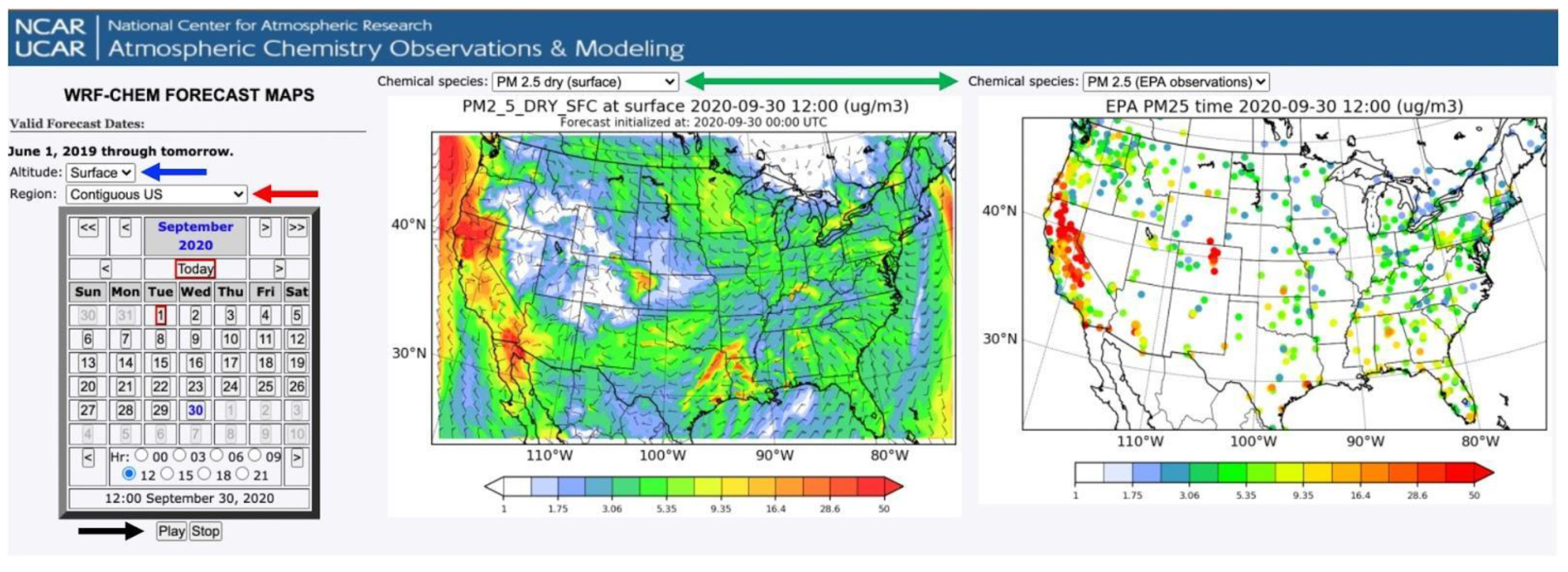
WRF-Chem forecasts are post-processed to generate many products that help fulfill the needs of the research community as well as air quality forecasters from the CDPHE. These products are displayed on the website “WRF-Chem Forecast maps” [29]. Figure 2 shows a snapshot of the information dissemination system. Users can display the spatial distribution of ozone, PM2.5, NOx, CO, CO source tracers, inert fire tracers, aerosol optical depth (AOD) at 550 nm, and key meteorological variables (planetary boundary layer height, downwelling solar radiation, relative humidity, and ventilation rate) for the CONUS, Colorado, and Colorado Front Range (a transition zone between the Great Plains and the Rocky Mountains in the central part of Colorado) at the surface and at 3 km, 5 km, and 8 km altitudes. The users can switch between the regions (red arrow in Figure 2), altitudes (blue arrow), and chemical species (green arrow) from the drop-down menus. We also display NRT observations of ozone and PM2.5 from the EPA AirNOW network for a qualitative NRT evaluation of our forecasts. Figure 2 shows an example of the comparison for PM2.5 for 30 September 2020 12 UTC over the CONUS. Both the model and observations show high PM2.5 along the western coast because of the California wildfires, but the model appeared to underestimate the observed PM2.5 levels at this time except in Minnesota, where the model slightly overestimated the observations.
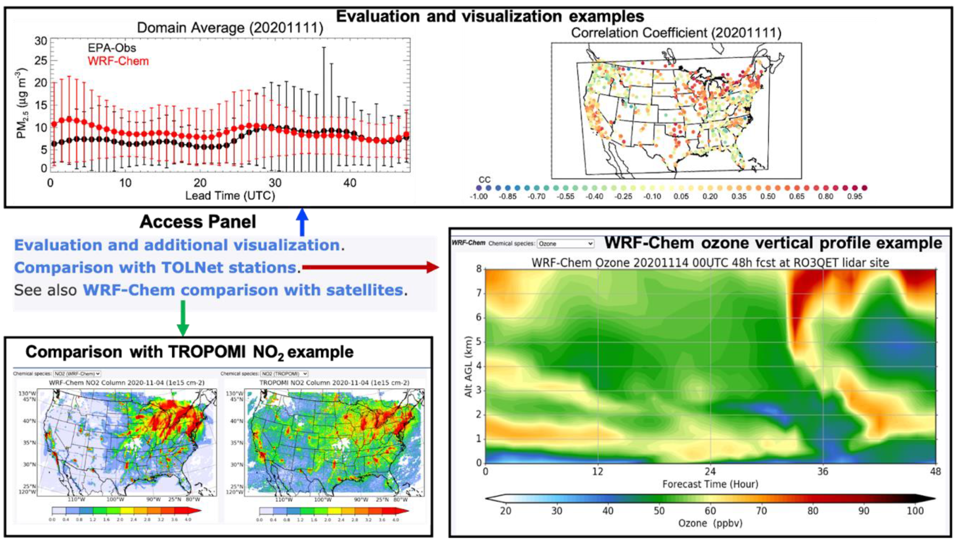
The website also hosts an access panel with links to evaluation and additional visualization, comparison with the TOLNET stations, and comparison to satellite retrievals (Figure 3). Under the evaluation and additional visualization, the users can access average statistics, hourly maps, Google Earth files (Keyhole Markup language Zipped (KMZ)) containing our forecasts, and forecasts at TOLNET sites. Average statistics include plots comparing the observed and forecasted time series of PM2.5 and ozone averaged over the CONUS, 10 EPA regions, Colorado, and the Front Range (see evaluation and visualization example in Figure 3). Maps for the CONUS showing correlation coefficient (r), mean bias (MB), and root mean squared error (RMSE) at each site for a given forecast cycle are also displayed. Hourly maps of the comparison of the model’s forecast with NRT observations are shown in Figure 2. Under the TOLNET link, we display the vertical profiles of ozone, CO, CO tracers, relative humidity, 300 nm backscatter coefficient, and 300 nm extinction coefficient for the full 48 h forecast cycle at all the TOLNET sites, i.e., Boulder, Greenbelt, Hampton, Huntsville, and Wrightwood (see Figure 3, bottom right panel for an example of ozone profile). A comparison of the WRF-Chem forecast against the Tropospheric Monitoring Instrument (TROPOMI) tropospheric column NO2 is provided on the website under the comparison with satellite data link (see bottom left panel of Figure 3 for an example).

3. Observations

Every day, we download hourly surface PM2.5 concentrations from 1136 EPA AirNOW sites for the NRT evaluation of our forecasts, as presented in Figure 2. These observations are downloaded with a 2-day lag so that a full forecast cycle can be validated. However, many of these sites have missing data, and for annual evaluation, we include only those sites that have valid data for at least 50% of the days in a month, and each day must have valid data for at least 18 h to be considered as a valid day. This requirement reduces the number of sites from 1136 to 612, of which 560 are located in the US. A map of the total sites and the sites used in this analysis is shown in the Supplementary Material (Figure S1). In addition, we use in situ observations of 2 m temperature and relative humidity, surface pressure, and 10 m wind speed and direction for the evaluation of the meteorological parameters simulated by WRF-Chem. The meteorological data used for this study is from the Aviation Routine Weather Record (METAR) network and is distributed by NCEP’s Meteorological Assimilation Data Ingest System (MADIS). The METAR data is a standard data record for reporting meteorological data in the US as part of a surface weather observation program. The METAR data has four different Quality Control (QC) checks, and in the model, we used level-3 QC-controlled data. For individual reporting sites (at QC = 3), there is a lot of missing METAR data. Similar to PM2.5 observations, we only include those sites that have valid data for at least 50% of the days in a month, and each day must have valid data for at least 18 h to be considered as a valid day. The total number of METAR sites that reported data during the study period was 1290, but the data validity requirement reduces the number of sites to 525, 513, 459, 516, 516, respectively, for 2 m temperature, relative humidity, surface pressure, 10 m wind speed and direction.

4. Results and Discussion

The model output is paired with the in-situ observations of near-surface temperature, pressure, relative humidity, wind speed, wind direction, and PM2.5 mass concentrations through bilinear interpolation to the observation site locations. The evaluation is performed in 10 regions defined by the EPA (see Supplementary Material, Figure S2 for region definition) to understand regional variability in model performance. Model performance is evaluated separately for the first and second days of the forecast to assess variations in the model performance as a function of the lead time.

4.1. Meteorological Evaluation

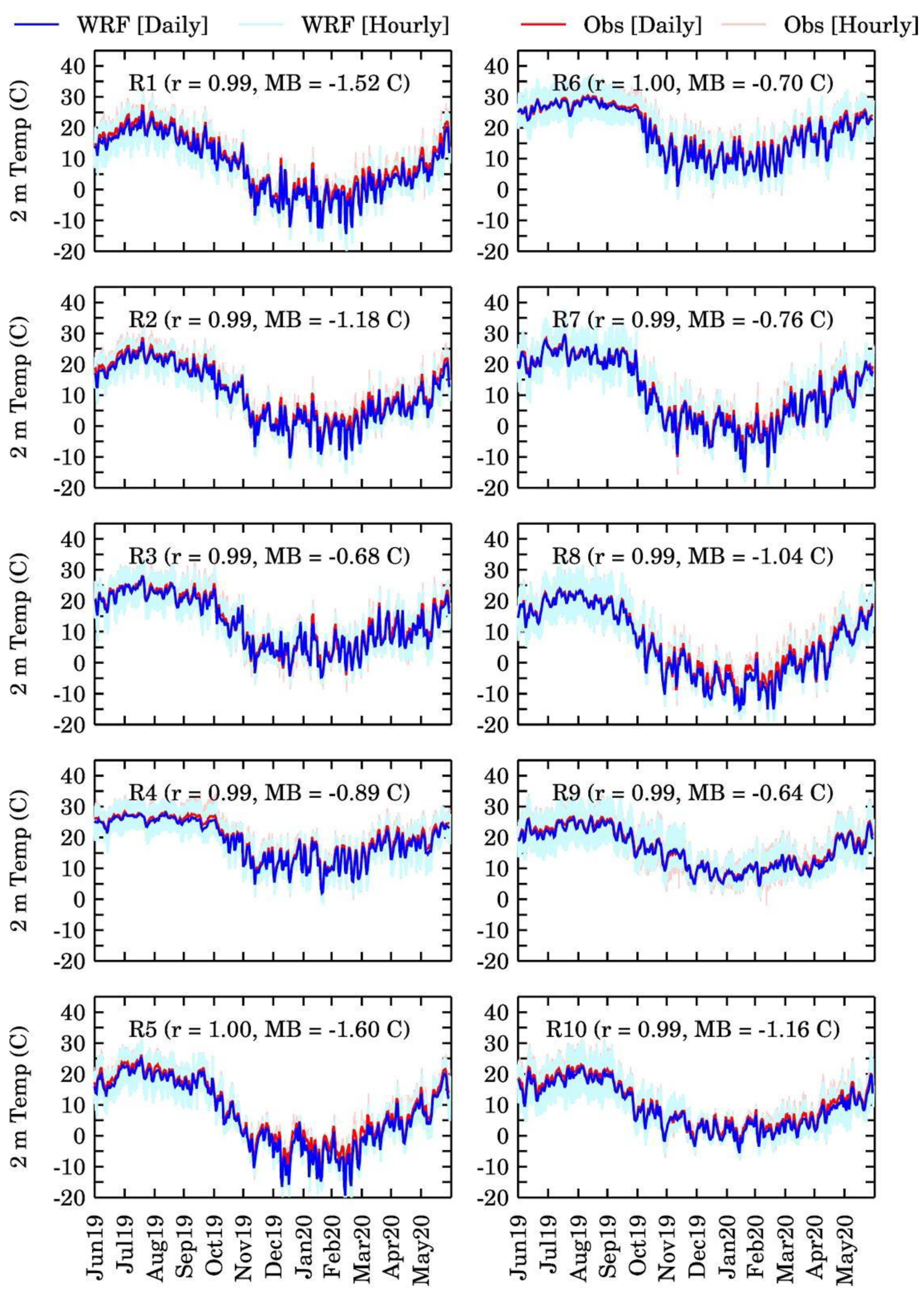
Figure 4 shows an evaluation of the modeled hourly and daily averaged 2 m temperature against the observations in the 10 EPA regions during June 2019 to May 2020 using paired data from the first day of each forecast cycle. The model showed an excellent ability to reproduce the observed seasonal cycle of 2 m temperature in all the regions and captures the seasonal cycle. The model also captured the regional variability in 2 m temperature with a lower amplitude of the seasonal cycle in the southern parts of the domain, i.e., R4, R6, and R9. The correlation coefficient between the model and observations in all the regions exceeded 0.99, and the mean bias was within ±1.6 K. We observed slightly higher differences between the model and observations in 2020 compared to 2019. This may have been because of the COVID-19 induced changes in anthropogenic emissions, which were not considered in our forecasting setup, and might feedback to the meteorology.
The model also showed an excellent ability to reproduce the hourly and daily averaged variations in surface pressure in the regions R1–R7 with correlation coefficients exceeding 0.98 and mean biases smaller than −3 hPa (Figure 5). However, the model showed poorer performance in the regions R8–R10, which includes the Rocky Mountains. The model could not resolve all the topographical features of the Rocky Mountains at a grid spacing of 12 km × 12 km, and the underestimation of surface pressure by the model in R8–R10 is reflective of the smoother topography used by the model. The mean bias in R9 and R10 went up to 7.5 hPa.
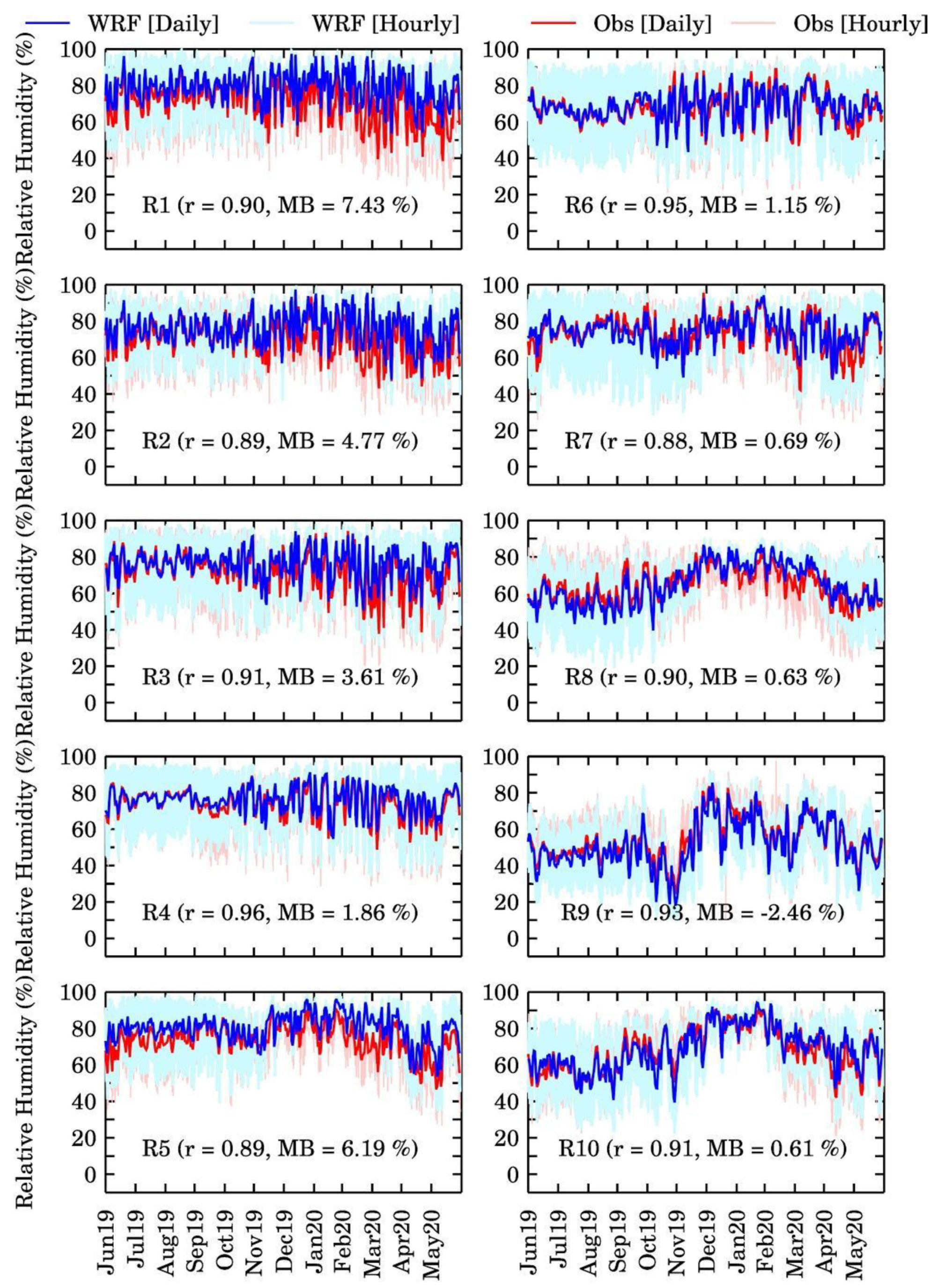
The model reproduced the observed seasonal cycle of relative humidity in all the regions with correlation coefficients exceeding 0.88 (Figure 6).
The model showed the largest errors in relative humidity (RH) in the R1, R2, and R5 regions. Interestingly, the model did not show large errors in the regions R9 and R10 where the model showed the highest errors in surface pressure. To analyze the effects of the bias seen in WRF simulated surface pressure (PSFC) in R8–R10, we analyzed the sensitivity of RH to variations in PSFC. WRF RH is derived from water vapor mixing ratio at 2 m (w), PSFC, and temperature at 2-m (T2) using the following equation from [30]
RH = ((PSFC × w)/((0.622 + w) × es(T2))) × 100  (%)
where es(T2) is the saturation vapor pressure at T2 and is derived using Equations (2) and (3):
es(T2) = 1013.25 × 10fact1
fact1 = 10.79586 × (1 − 273.15/T2) − 5.02808 × alog10(T2/273.15) + 1.50474 ×
10−4 × (1 − 10(−8.29692 × (T2/273.15 − 1))) + 0.42873 × 10−3 × (10(4.76955 × (1 − 273.15/T2)) − 1) −
2.2195983
At a constant w, the biases in PSFC and T2 will determine the error in RH. The maximum mean bias values in PFSC and T2 for all the regions were estimated as 7.5 hPa and 1.6 °C, respectively. To assess the impact of these biases on RH calculation, we also calculated RH by adding ±3.5 hPa and ±0.8 °C to PSFC and T2, respectively. The changes in RH due to surface pressure perturbations were estimated at 0.6%, 0.4%, and 0.6% for the regions R8, R9, and R10, respectively. In contrast, temperature perturbations caused larger changes in RH of −7.6%, −5.5%, and −7.7% for the regions R8, R9, and R10, respectively. Thus, the RH calculation was more sensitive to temperature bias rather than the pressure bias, and that is why the modeled and observed RH had a reasonable agreement in regions R8–R10 despite the bias in surface pressure.
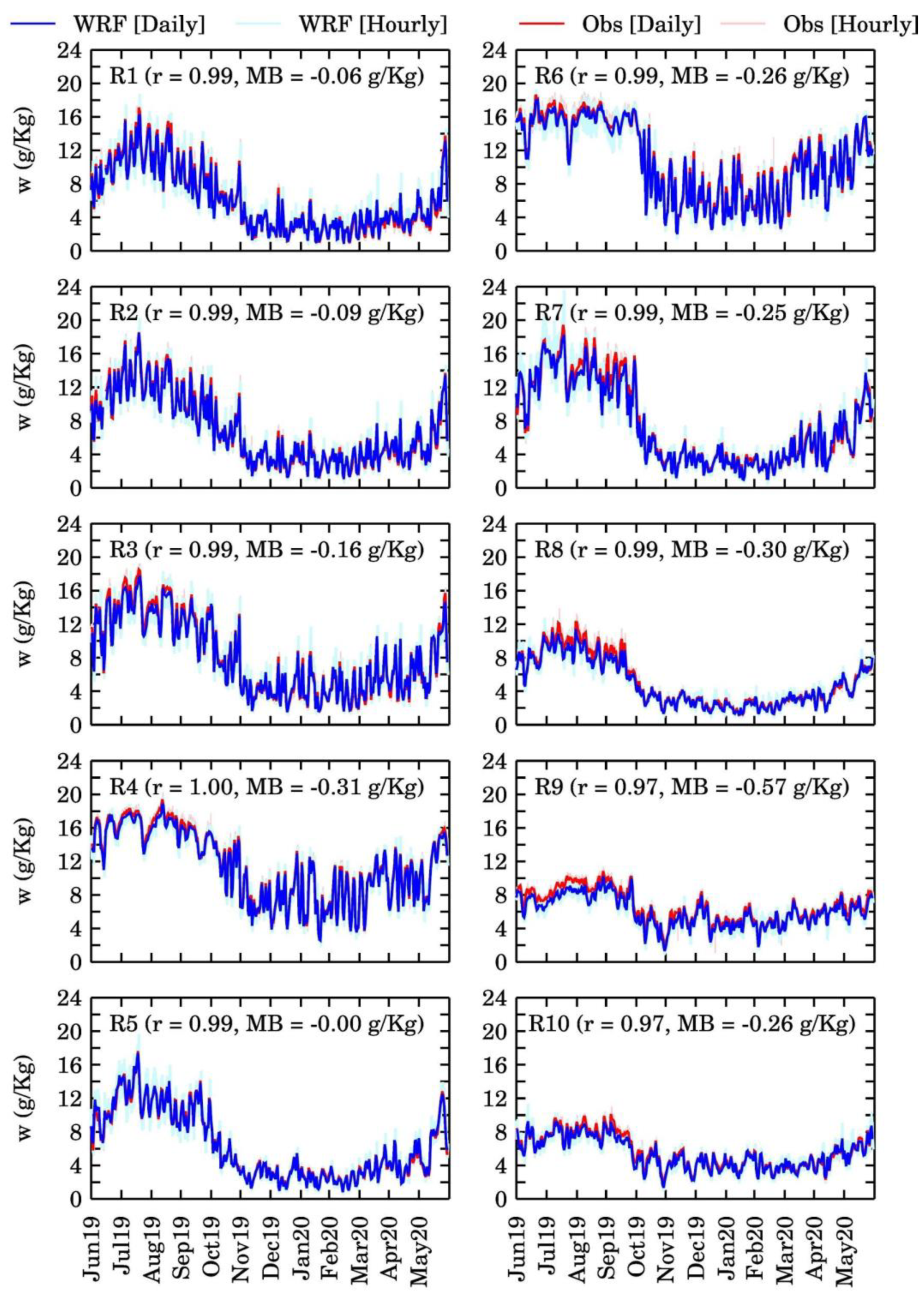
Since water vapor mixing ratios (w) also determine the RH, we calculated w from the dew point temperature (Td) and PSFC using Equation (4)
w = (0.622 × e(Td)/(PSFC − e(Td))  (Kg/Kg)
e(Td) = 1013.25 × 10fact2
fact2 = 10.79586 × (1 − 273.15/Td) − 5.02808 × alog10(Td/273.15) + 1.50474 × 10−4
× (1 − 10(−8.29692 × (Td/273.15 – 1))) + 0.42873 × 10−3 × (10(4.76955 × (1 − 273.15/Td)) − 1) − 2.2195983
where e(Td) is vapor pressure and is estimated using Equations (5) and (6) provided by [30]. The comparison of the seasonal cycle of WRF and METAR derived w for day-1 forecasts is shown in Figure 7. The model captured the seasonal cycle of w very well in all the regions as indicated by r values exceeding 0.97 and mean biases smaller than 0.57 g/kg. The good comparison between WRF and METAR water vapor mixing ratios and higher sensitivity to temperature errors indicated that higher biases in RH in the latter half of the study period in R1–R3 and R5 were likely a result of larger errors in temperature. To confirm this, we estimated RH using WRF PSFC, WRF w, and observed METAR T2. This revised RH (rev) estimated by eliminating the temperature bias showed (Figure S3) a lower mean bias than the WRF RH (derived from WRF T2).
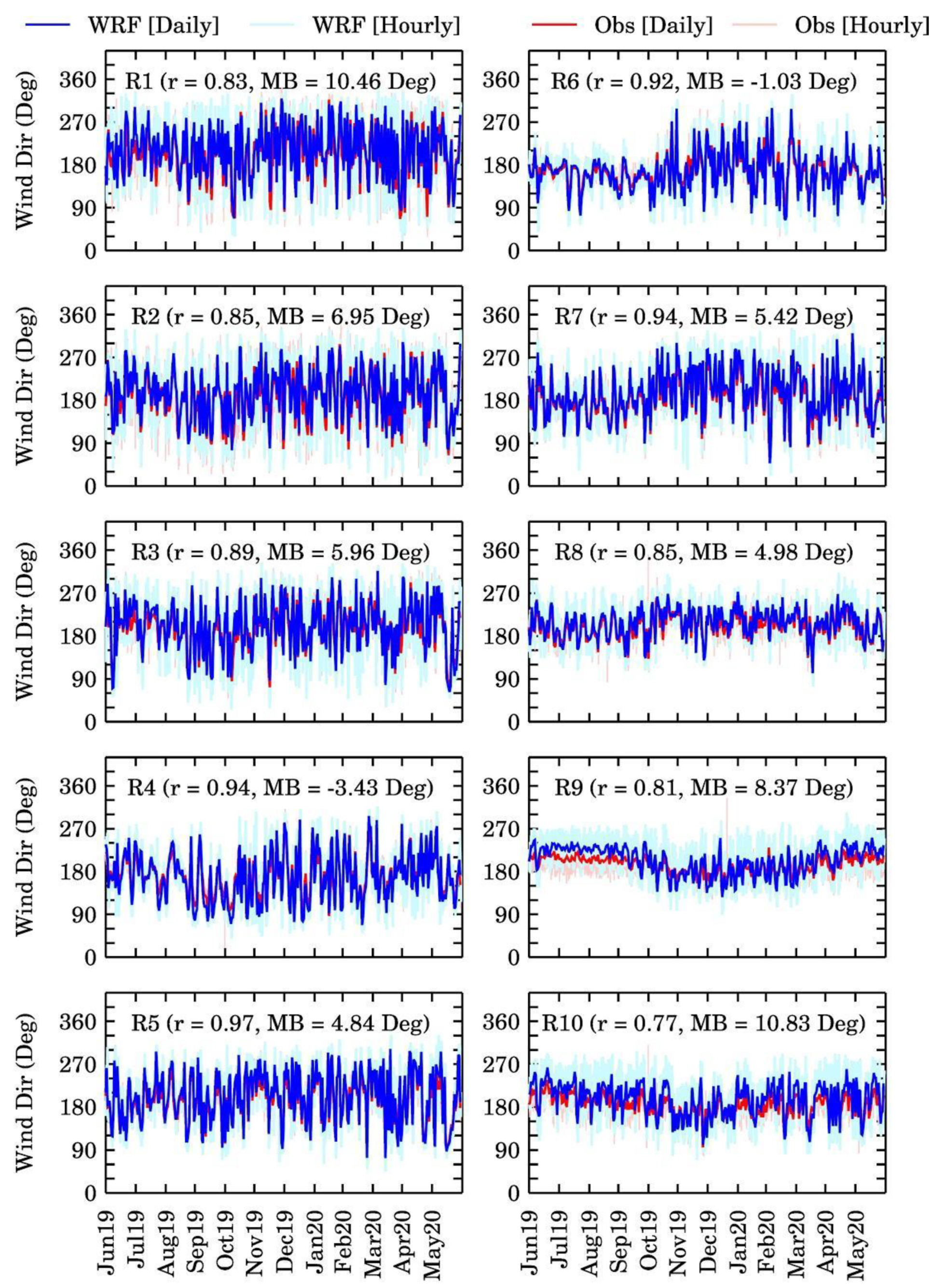
For the appropriate evaluation of the modeled 10 m wind speed, we replaced all instances of calm winds (wind speed less than 1 knot) in the model by zero, as is done in the METAR dataset. The model captured the observed seasonal changes in 10 m wind speed in all the regions but generally overestimated the wind speed by 0.64–1.06 m/s on average (Figure 8). The correlation coefficients for 10 m wind speed were lower than those for temperature, pressure, and relative humidity, indicating a slightly poorer model performance for winds. The WRF model is well known to overpredict 10 m wind speed at low to moderate wind speeds in all available planetary boundary layer (PBL) schemes [31]. This shortcoming of the model was partly attributed to unresolved topographical features by the default surface drag parameterization, which in turn influences surface drag and friction velocity and partly to the use of coarse horizontal and vertical resolutions of the domain [32]. Mass and Ovens [31] also found this overestimation at the horizontal grid spacing of 4 km × 4 km but noticed improvement at 1.3 km × 1.3 km grid spacing. In contrast to wind speed, the model captured the wind direction in all the regions very well, with correlation coefficients exceeding 0.77 and mean biases within 11° (Figure 9).
The model performance for second-day forecasts is presented in the Supplementary Material (Figures S4–S9) and was very similar to the first-day forecasts. The range of statistical parameters for the first- and second-day forecasts for all the meteorological parameters are shown in Table 2. It can be clearly seen that these statistical metrics did not change significantly from the first- to second-day of forecasting except for the wind speed, where we saw large differences in the correlation coefficient from the first to the second day of the forecast. These results suggest that the meteorological accuracy of our forecasting system does not change significantly with the lead time.

4.2. Surface PM2.5 Evaluation

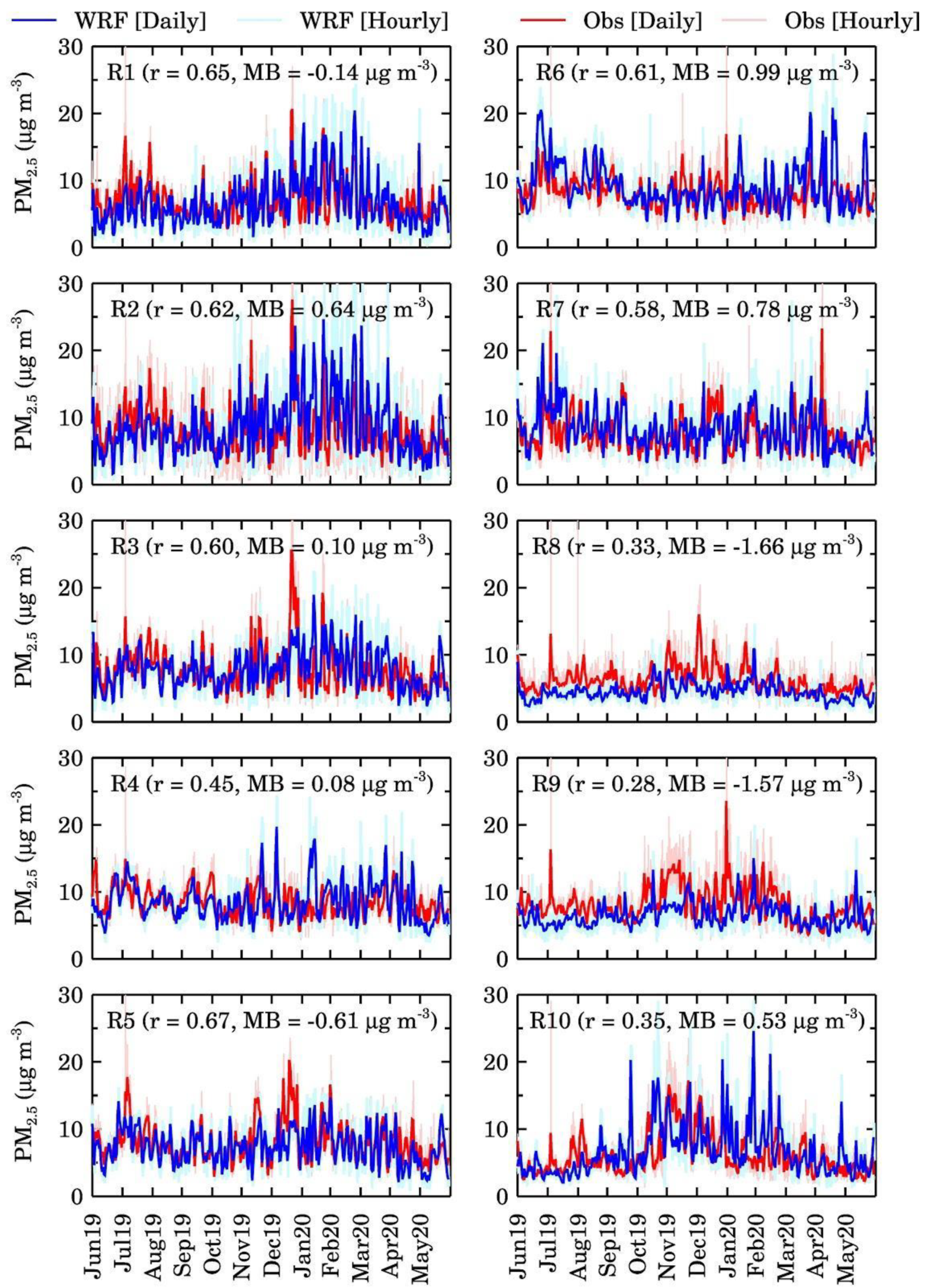
The variations in hourly and daily averaged WRF-Chem forecasted surface PM2.5 mass concentrations were evaluated against the EPA AirNOW observations from 1 June 2019 to 31 May 2020 (see Figure 10 for the first-day forecasts and Figure S10 for the second-day forecast). In most of the EPA regions, both the model and observations showed the highest surface PM2.5 during the winter season. Higher wintertime PM2.5 mass concentrations can be attributed to two factors. First, the seasonal cycle of anthropogenic emissions (see Figure S11) showed that OC emissions peaked in winter in almost all the regions, which was likely due to residential wood burning. Second, the boundary layer was shallower during the winter, and the emissions were trapped into a smaller volume near the surface. In contrast, a deeper boundary layer during summer combined with injection of fire emissions into the free troposphere leads to lower surface PM2.5 mass concentrations during summer. Forest fires generally play an important role, but 2019 was a low fire activity year. To understand the relative roles of anthropogenic and fire emissions, we also analyzed the time series of carbon monoxide (CO) tracers implemented to track CO emitted from anthropogenic (CO (Anth)) and fire (CO (Fire)) emissions in our forecasts. The seasonal cycle of CO (Anth) and CO (fire) is shown in Figure S12. CO (Fire) was always less than CO (Anth), indicating that fire emissions overall did not play a dominant role in controlling air quality during our study period.
WRF-Chem showed a moderate ability to capture the seasonal cycle of surface PM2.5 mass concentrations in the R1–R3 and R5–R7 regions with the correlation coefficient exceeding 0.58 but performed poorly in the remaining regions, i.e., R4 and R8–R10. The annual mean bias in different regions is within ±2 µg m−3, with the highest bias in the R8 and R9 regions. However, the daily mean bias occasionally exceeded 20 µg m−3 in some of the regions. The underestimation of PM2.5 by the model could be partly attributed to the use of the MOZCART chemical mechanism in WRF-Chem, which is linked to the GOCART aerosol scheme. The GOCART scheme does not include nitrate and secondary organic aerosols and thus is missing some of the aerosol components. In addition, wildfire aerosol emissions in FINN v1 are known to be biased low and are expected to contribute to the low model results as well. To understand the model performance in different environments, we also evaluated the model performance in simulating PM2.5 at urban (Figure S13), suburban (Figure S14), and rural (Figure S15) site types. The model performance at the urban, suburban, and rural sites was overall similar to the performance at all sites. The largest mean bias at all types of sites was noticed in regions R8 and R9. The urban sites showed the largest mean bias in region R8, whereas the suburban and rural sites showed the largest mean bias in region R9. The range of statistical scores across the 10 EPA regions for PM2.5 performance at all sites, urban, suburban, and rural sites for day 1 and day 2 forecasts are also shown in Table 2. The statistical scores at all types of sites did not change significantly from the first to the second day of the forecast, indicating that the model’s performance remained fairly constant over the forecast duration.
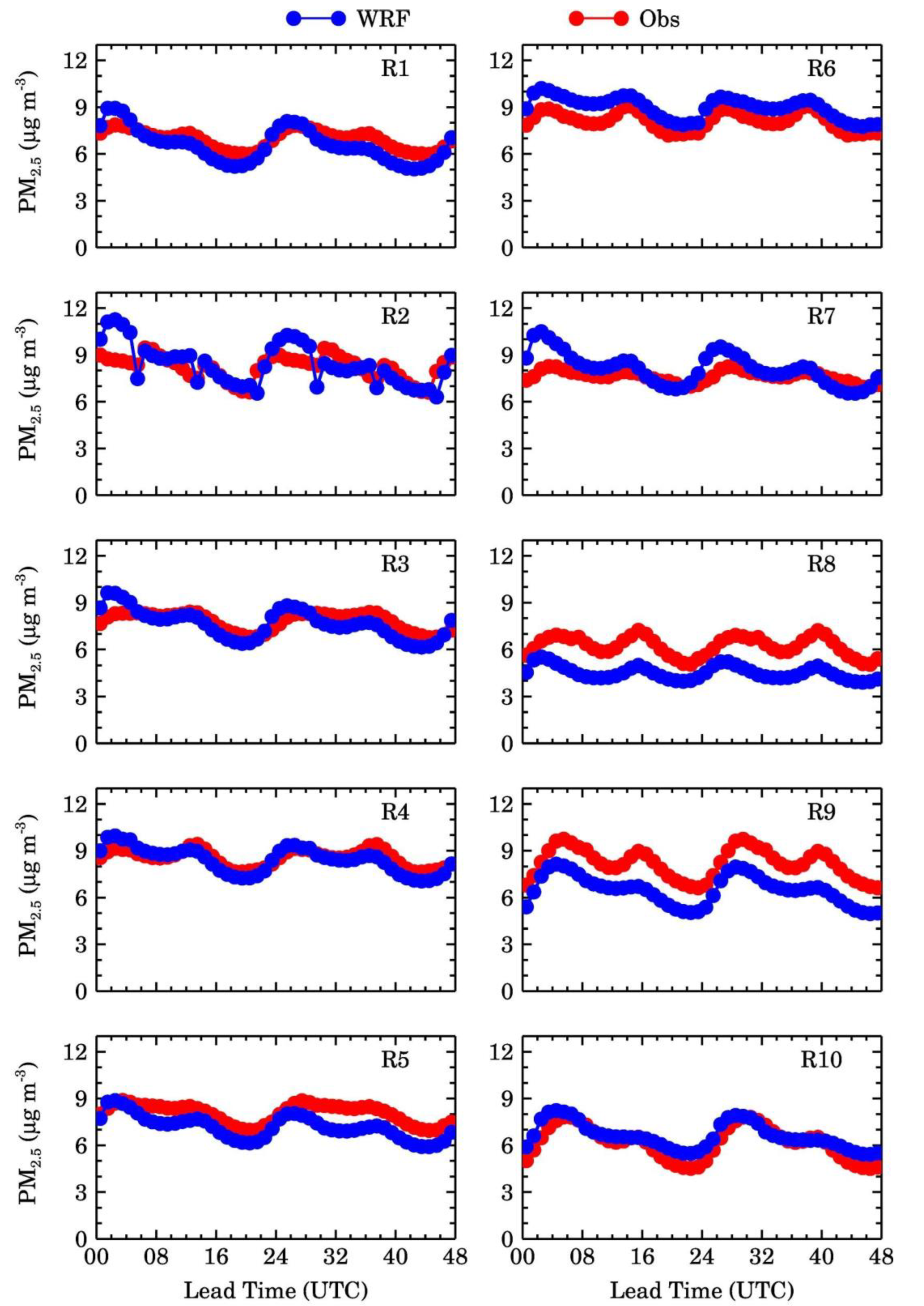
To provide further insight into the hourly performance of our forecasts, we compared the time series of forecasted and observed PM2.5 mass concentrations on a 48 h time scale obtained by averaging paired data from all the sites in each EPA region (Figure 11). In all the regions, our forecasts captured higher nighttime and lower daytime concentrations of PM2.5. This diurnal variability in PM2.5 mass concentrations results from a combination of the diurnal variations in emissions and boundary layer dynamics. The hourly standard deviation (not shown in Figure 11) averaged observed values (3.73–10.09 µg/m3) was slightly higher than using the model (3.36–8.94 µg/m3). The difference between the model and observations slightly increases with lead time in regions R1, R4, R5, and R8, whereas it either stayed constant or slightly decreased in other regions.
We also analyzed the daily variations in the Pearson’s correlation coefficient (r), mean bias (MB), and root mean squared error (RMSE). These statistical metrics were calculated from model-observations pairs available at all the sites over the 48 h forecast period every day in each EPA region. Daily variations in r, MB, and RMSE in each EPA region are shown in Figures S16–S18, respectively. We noticed a large day-to-day variability in all the statistical parameters with r, MB, and RMSE values ranging from −0.43–0.88, −11.97–16.05 µg/m3, and 2.13–36.06 µg/m3, respectively. The highest r values were seen in R1–R3 (i.e., the eastern US), and the lowest r values were seen in R8–R10 (i.e., the western US). The mean bias changes were from mostly negative in summer to mostly positive in winter and early spring, particularly in regions R1–R4. The mean bias was mostly within ±5 µg/m3 in regions R5–R7 and was mostly negative throughout the year in R8 and R9. The mean bias fluctuated more rapidly between negative and positive values in R10. The RMSE shows an increase during winter in R1, R2, and R8–R10, while the other regions showed a relatively constant RMSE throughout the year along with some occasional increase in the RMSE. We also attempted to analyze daily variations in these statistical metrics for high aerosol loading events characterized by daily average PM2.5 mass concentrations, but very limited occurrences of such events inhibited us from investigating the daily regional variability in these metrics during such events.
These seasonal changes in the model performance can be attributed to several factors, including uncertainties in the seasonal cycle and magnitude of the emissions, changes in nitrate and SOA aerosols across regions and seasons which are not simulated by the GOCART scheme, errors in meteorological and chemical initialization of the model, errors in physical parameterizations that can lead to errors in PBL dynamics, chemical kinetics, and deposition, and the inability of the model to resolve complex topographical features. For example, recent studies have shown that an average change of about 1.5 µg/m3 in initial conditions can change 48 h PM2.5 forecasts by 0.5–3 µg/m3 at different lead times in the US [33,34]. The horizontal grid spacing is also shown to affect model simulations, particularly in urban, coastal, and complex terrain regions [35]. Uncertainties in dry deposition parameterizations are estimated to introduce an uncertainty of up to 40% on anthropogenic and 52% on biogenic organic aerosols over CONUS in the WRF-Chem model [36,37].
To understand which chemical species contribute the most to PM2.5 mass concentrations in different regions, we analyzed the mass concentration of black carbon (BC), organic carbon (OC), dust, sea-salt, sulfate, and other PM2.5. For the GOCART model, the PM2.5 mass concentrations were calculated using the following equation
PM2.5 = BC1 + BC2 + (OC1 + OC2) × 1.8 + DUST1 + 0.286 × DUST2 + SEAS1 +
0.942 × SEAS2 + 1.375 × SULF + P25
where BC1 and BC2 represent hydrophobic and hydrophilic BC, respectively; OC1 and OC2 represent hydrophobic and hydrophilic OC, respectively; P25 represents non-speciated primary PM2.5, DUST1 and DUST2 represent dust from the first and second bins corresponding to effective radii of 0.73 µm and 1.4 µm, respectively; SEAS1 and SEAS2 represent sea-salt from the first and second bins corresponding to effective radii of 0.3 µm and 1.0 µm, respectively; SULF represents sulfate. SULF was multiplied by 1.375, which is the ratio of molecular weight of ammonium sulfate (132.14 g/mol) to sulfate (96.06 g/mol). Since GOCART assumes that sulfate aerosols are present as ammonium sulfate, multiplication of SULF by 1.375 adds the missing ammonium mass needed to neutralize sulfate. (OC1 + OC2) was multiplied by 1.8 to convert organic carbon to organic matter.
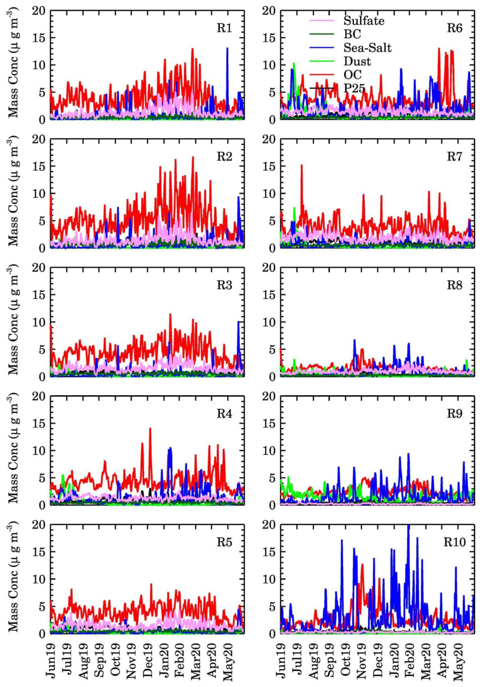
The values of all the aerosol chemical components contributing to PM2.5 mass concentration at the EPA AirNOW sites were extracted from the six hourly model output. The variations in daily averaged BC, OC, Dust, Sea-salt, and P25, and Sulfate in 10 EPA regions are presented in Figure 12. OC was the most dominant contributor to PM2.5 mass concentration in regions R1–R7, with Sulfate and sea-salt becoming the other two most important contributors. Dust also appeared as an important contributor to total PM2.5 in R6 in June 2019. Dust, sea-salt, OC, and Sulfate were the most important contributors to PM2.5 mass concentration in regions R8 and R9, while OC and sea-salt were the most important in region R10.
To understand this regional variability in PM2.5 composition, we analyzed the seasonal cycle of the U.S. NEI 2014 anthropogenic emissions of BC, OC, SO2, and other unspeciated PM2.5 (P25) used in the model in each EPA region (Figure S11). In most of the regions, OC emissions were the highest in almost all regions except during June–October in regions R7–R10, where OC and P25 emissions were comparable, and throughout the year in R6. Higher OC emissions explain the dominance of OC contribution to PM2.5 composition. Dust emissions are calculated online within the model and are not output in our forecasts. To understand why dust concentrations were the highest in R9, we show the spatial distribution of the dust source function in Figure S19. The dust source function represents the fraction of alluvium available for wind erosion and thus marks the grid boxes from where dust can be emitted. Dust source functions are pre-calculated and provided as a fixed input dataset to the model. In California, Nevada, and Arizona, which have the highest dust source function and all belong to region R9; we saw the highest dust concentrations in that region.

5. Conclusions and Outlook

This paper presents the setup, configuration, and evaluation of the surface PM2.5 and meteorological components of the NCAR regional air quality forecasting system. The system complements the NOAA operational air quality forecasts by providing an additional piece of information for decision-makers, and the public serves as a testbed for identifying errors and biases in the model performance through NRT evaluation, supports field campaign planning, and provides the atmospheric chemistry community a data set to support their research needs. The model shows excellent skill in capturing hourly to daily variations in temperature, surface pressure, relative humidity, and wind direction but showed relatively larger errors in wind speed. The model also captures the seasonal cycle of surface PM2.5 observations very well in all different regions of the US with a mean bias smaller than 1 µg m−3. The skill of the forecasting system in simulating both the meteorological parameters and PM2.5 mass concentrations does not change significantly from the first to the second day of the forecast. While the model shows a reasonable performance in capturing daily variations, the model is overall underestimating concentrations on days when PM2.5 exceeds its National Ambient Air Quality Standard. To a large degree, this is due to the model not simulating nitrate aerosols and SOA but also because of the 12 km spatial resolution. Hence, for any forecast model that uses a simplified aerosol scheme, these shortcomings need to be considered in the interpretation.
We plan to take several steps in the coming years to further improve the accuracy of the air quality forecasts in our system. First, we plan to replace the monthly averaged anthropogenic emissions with weekday and weekend/holiday varying anthropogenic emissions and also adjust the emissions for the non-NEI reported years using the EPA reported annual trends in emissions. Second, we plan to initialize our air quality forecasts via the assimilation of Moderate Resolution Imaging Spectroradiometer (MODIS) AOD retrievals, which have been found very useful in reducing biases in Community Multiscale Air Quality (CMAQ) model predictions of PM2.5 over the CONUS [33] and WRF-Chem predictions of PM2.5 in Delhi [12]. Third, we plan to evaluate how well the persistence fire assumption works in the CONUS and whether we can develop an algorithm to predict fire emissions for two days in the future possibilities based on machine learning techniques. Future fire emissions can be predicted using fire behavior and spread models, but they are computationally too intensive to be applied to a large number of fires that can be detected in a given day over the CONUS. Future studies will also present a comprehensive evaluation of surface ozone and related species against the available in situ and satellite-based observations. Finally, we invite the community to use our forecasting products to join in the analysis, use the model output as boundary conditions for finer scale (~4 km grid spacing) air quality forecasts over urban areas of CONUS, or co-develop customized products to serve their needs.

Supplementary Materials

The following are available online at https://www.mdpi.com/2073-4433/12/3/302/s1, Figure S1: Map of all PM2.5 observation sites (black dots) used in near-real-time verification and the sites (red dots) used in the annual evaluation presented in this study. Figure S2: Definition of EPA regions. Figure reproduced from the EPA regional website (https://www.epa.gov/aboutepa/visiting-regional-office (accessed on 20 February 2021)). Figure S3: Seasonal variations in daily observed (Obs) model simulated (WRF) and revised (Rev) 2 m relative humidity in four EPA regions during June 2019 to May 2020. r and MB for each region estimated using paired data for the full year are also shown. Figure S4: Same as Figure 4 but using day 2 of the forecast. Figure S5: Same as Figure 5 but using day 2 of the forecast. Figure S6: Same as Figure 6 but using day 2 of the forecast. Figure S7: Same as Figure 7 but using day 2 of the forecast. Figure S8: Same as Figure 8 but using day 2 of the forecast. Figure S9: Same as Figure 9 but using day 2 of the forecast. Figure S10: Same as Figure 10 but using day 2 of the forecast. Figure S11: Monthly variations in BC, OC, P25, and SO2 emissions averaged at the EPA AirNOW observation sites in each EPA region. BC, OC, and P25 emissions are in ng m−2 s−1, and SO2 emissions are in mole km−2 h−1. Figure S12: Variations in daily averaged CO (Anth) and CO (Fire) tracers in 10 EPA regions from 1 June 2019 to 31 May 2020. Figure S13: Variations in hourly and daily averaged WRF-Chem forecasted surface PM2.5 mass concentrations against the EPA AirNOW observations at the urban sites in 10 EPA regions from 1 June 2019 to 31 May 2020. r and MB for each region estimated using paired data for the full year are also shown. Figure S14: Same as Figure S13 but at the suburban sites. Figure S15: Same as Figure S13 but at the rural sites. Figure S16: Seasonal variations in the Pearson’s correlation coefficient (r) calculated from model-observations pairs available at all the sites over the 48-h forecast period every day in each EPA region. Figure S17: Seasonal variations in the mean bias (MB) calculated from model-observations pairs available at all the sites over the 48-h forecast period every day in each EPA region. Figure S18: Seasonal variations in the root mean squared error (RMSE) calculated from model-observations pairs available at all the sites over the 48-h forecast period every day in each EPA region. Figure S19: Spatial distribution of the dust source function over the model domain.

Author Contributions

Conceptualization, R.K. and G.P.; methodology, R.K., G.P., P.B. and C.D.; software, R.K., G.P., P.B., S.H., C.D. and G.D.; validation, R.K., G.P. and P.B.; formal analysis, R.K., G.P. and P.B.; data curation, C.D., S.H. and G.D.; writing—original draft preparation, R.K.; writing—review and editing, R.K., G.P., P.B., S.H., C.D. and G.D.; visualization, R.K., P.B., C.D. and G.D.; supervision, R.K. and G.P.; project administration, G.P.; funding acquisition, R.K. and G.P.; All authors have read and agreed to the published version of the manuscript.

Funding

This research was funded by NASA, grant number 80NSSC18K0681, and the European Commission, grant number 870301.

Institutional Review Board Statement

Not applicable.

Informed Consent Statement

Not applicable.

Data Availability Statement

The model output used in this study are archived at the NCAR campaign storage and can be accessed by contacting the corresponding authors. All the meteorological and chemical observations used in the study are publicly available. The meteorological data is available at https://madis-data.cprk.ncep.noaa.gov/madisPublic1/data/archive/ (accessed on 20 February 2021). The air quality observations are available from the EPA Air Quality System at https://www.epa.gov/aqs (accessed on 20 February 2021).

Acknowledgments

We acknowledge the use of near-real-time US EPA AirNow surface monitoring data. We would like to acknowledge high-performance computing support from Cheyenne (doi: 10.5065/D6RX99HX (accessed on 20 February 2021)(accessed on 20 February 2021)), provided by NCAR’s Computational and Information Systems Laboratory, sponsored by the National Science Foundation. We acknowledge the use of the WRF-Chem preprocessor tool anthro_emis provided by the Atmospheric Chemistry Observations and Modeling Laboratory (ACOM) of NCAR. The National Center for Atmospheric Research is sponsored by the National Science Foundation. We thank the three anonymous reviewers and the academic editor for their constructive comments on the manuscript, which have helped improve the quality of the manuscript.

Conflicts of Interest

The authors declare no conflict of interest. The funders had no role in the design of the study, in the collection, analyses, interpretation of data, in the writing of the manuscript, or in the decision to publish the results.

References

  1. Burnett, R.T.; Pope, C.A.; Ezzati, M.; Olives, C.; Lim, S.S.; Mehta, S.; Shin, H.H.; Singh, G.; Hubbell, B.; Brauer, M.; et al. An Integrated Risk Function for Estimating the Global Burden of Disease Attributable to Ambient Fine Particulate Matter Exposure. Environ. Health Perspect. 2014, 122, 397–403. [Google Scholar] [CrossRef]
  2. Fann, N.; Lamson, A.D.; Anenberg, S.C.; Wesson, K.; Risley, D.; Hubbell, B.J. Estimating the National Public Health Burden Associated with Exposure to Ambient PM2.5 and Ozone. Risk Anal. 2012, 32, 81–95. [Google Scholar] [CrossRef]
  3. Di, Q.; Wang, Y.; Zanobetti, A.; Wang, Y.; Koutrakis, P.; Choirat, C.; Dominici, F.; Schwartz, J.D. Air Pollution and Mortality in the Medicare Population. New Engl. J. Med. 2017, 376, 2513–2522. [Google Scholar] [CrossRef]
  4. Im, U.; Brandt, J.; Geels, C.; Hansen, K.M.; Christensen, J.H.; Andersen, M.S.; Solazzo, E.; Kioutsioukis, I.; Alyuz, U.; Balzarini, A.; et al. Assessment and Economic Valuation of Air Pollution Impacts on Human Health over Europe and the United States as Calculated by a Multi-Model Ensemble in the Framework of AQMEII3. Atmos. Chem. Phys. 2018, 18, 5967–5989. [Google Scholar] [CrossRef] [PubMed] [Green Version]
  5. Lee, P.; McQueen, J.; Stajner, I.; Huang, J.; Pan, L.; Tong, D.; Kim, H.; Tang, Y.; Kondragunta, S.; Ruminski, M.; et al. NAQFC Developmental Forecast Guidance for Fine Particulate Matter (PM2.5). Weather Forecast. 2017, 32, 343–360. [Google Scholar] [CrossRef]
  6. Chouza, F.; Leblanc, T.; Brewer, M.; Wang, P.; Piazzolla, S.; Pfister, G.; Kumar, R.; Drews, C.; Tilmes, S.; Emmons, L. The Impact of Los Angeles Basin Pollution and Stratospheric Intrusions on the Surrounding San Gabriel Mountains as Seen by Surface Measurements, Lidar, and Numerical Models. Atmos. Chem. Phys. Discuss. 2020, 1–29. [Google Scholar] [CrossRef]
  7. Grell, G.A.; Peckham, S.E.; Schmitz, R.; McKeen, S.A.; Frost, G.; Skamarock, W.C.; Eder, B. Fully Coupled “Online” Chemistry within the WRF Model. Atmos. Environ. 2005, 39, 6957–6975. [Google Scholar] [CrossRef]
  8. Powers, J.G.; Klemp, J.B.; Skamarock, W.C.; Davis, C.A.; Dudhia, J.; Gill, D.O.; Coen, J.L.; Gochis, D.J.; Ahmadov, R.; Peckham, S.E.; et al. The Weather Research and Forecasting Model: Overview, System Efforts, and Future Directions. Bull. Am. Meteorol. Soc. 2017, 98, 1717–1737. [Google Scholar] [CrossRef]
  9. Marsh, D.R.; Mills, M.J.; Kinnison, D.E.; Lamarque, J.-F.; Calvo, N.; Polvani, L.M. Climate Change from 1850 to 2005 Simulated in CESM1(WACCM). J. Clim. 2013, 26, 7372–7391. [Google Scholar] [CrossRef] [Green Version]
  10. Wiedinmyer, C.; Akagi, S.K.; Yokelson, R.J.; Emmons, L.K.; Al-Saadi, J.A.; Orlando, J.J.; Soja, A.J. The Fire INventory from NCAR (FINN): A High Resolution Global Model to Estimate the Emissions from Open Burning. Geosci. Model. Dev. 2011, 4, 625–641. [Google Scholar] [CrossRef] [Green Version]
  11. Freitas, S.R.; Longo, K.M.; Chatfield, R.; Latham, D.; Silva Dias, M.A.F.; Andreae, M.O.; Prins, E.; Santos, J.C.; Gielow, R.; Carvalho, J.A., Jr. Including the Sub-Grid Scale Plume Rise of Vegetation Fires in Low Resolution Atmospheric Transport Models. Atmos. Chem. Phys. 2007, 7, 3385–3398. [Google Scholar] [CrossRef] [Green Version]
  12. Kumar, R.; Ghude, S.D.; Biswas, M.; Jena, C.; Alessandrini, S.; Debnath, S.; Kulkarni, S.; Sperati, S.; Soni, V.K.; Nanjundiah, R.S.; et al. Enhancing Accuracy of Air Quality and Temperature Forecasts During Paddy Crop Residue Burning Season in Delhi Via Chemical Data Assimilation. J. Geophys. Res. Atmos. 2020, 125, e2020JD033019. [Google Scholar] [CrossRef]
  13. Guenther, A.B.; Jiang, X.; Heald, C.L.; Sakulyanontvittaya, T.; Duhl, T.; Emmons, L.K.; Wang, X. The Model of Emissions of Gases and Aerosols from Nature Version 2.1 (MEGAN2.1): An Extended and Updated Framework for Modeling Biogenic Emissions. Geosci. Model. Dev. 2012, 5, 1471–1492. [Google Scholar] [CrossRef] [Green Version]
  14. Guenther, A.; Karl, T.; Harley, P.; Wiedinmyer, C.; Palmer, P.I.; Geron, C. Estimates of Global Terrestrial Isoprene Emissions Using MEGAN (Model of Emissions of Gases and Aerosols from Nature). Atmos. Chem. Phys. 2006, 6, 3181–3210. [Google Scholar] [CrossRef] [Green Version]
  15. Ginoux, P.; Chin, M.; Tegen, I.; Prospero, J.M.; Holben, B.; Dubovik, O.; Lin, S.-J. Sources and Distributions of Dust Aerosols Simulated with the GOCART Model. J. Geophys. Res. Atmos. 2001, 106, 20255–20273. [Google Scholar] [CrossRef]
  16. Gong, S.L.; Barrie, L.A.; Blanchet, J.-P. Modeling Sea-Salt Aerosols in the Atmosphere: 1. Model Development. J. Geophys. Res. Atmos. 1997, 102, 3805–3818. [Google Scholar] [CrossRef] [Green Version]
  17. Emmons, L.K.; Walters, S.; Hess, P.G.; Lamarque, J.-F.; Pfister, G.G.; Fillmore, D.; Granier, C.; Guenther, A.; Kinnison, D.; Laepple, T.; et al. Description and Evaluation of the Model for Ozone and Related Chemical Tracers, Version 4 (MOZART-4). Geosci. Model. Dev. 2010, 3, 43–67. [Google Scholar] [CrossRef] [Green Version]
  18. Chin, M.; Ginoux, P.; Kinne, S.; Torres, O.; Holben, B.N.; Duncan, B.N.; Martin, R.V.; Logan, J.A.; Higurashi, A.; Nakajima, T. Tropospheric Aerosol Optical Thickness from the GOCART Model and Comparisons with Satellite and Sun Photometer Measurements. J. Atmos. Sci. 2002, 59, 461–483. [Google Scholar] [CrossRef]
  19. Chin, M.; Rood, R.B.; Lin, S.-J.; Müller, J.-F.; Thompson, A.M. Atmospheric Sulfur Cycle Simulated in the Global Model GOCART: Model Description and Global Properties. J. Geophys. Res. Atmos. 2000, 105, 24671–24687. [Google Scholar] [CrossRef]
  20. Thompson, G.; Field, P.R.; Rasmussen, R.M.; Hall, W.D. Explicit Forecasts of Winter Precipitation Using an Improved Bulk Microphysics Scheme. Part II: Implementation of a New Snow Parameterization. Mon. Weather Rev. 2008, 136, 5095–5115. [Google Scholar] [CrossRef]
  21. Iacono, M.J.; Delamere, J.S.; Mlawer, E.J.; Shephard, M.W.; Clough, S.A.; Collins, W.D. Radiative Forcing by Long-Lived Greenhouse Gases: Calculations with the AER Radiative Transfer Models. J. Geophys. Res. Atmos. 2008, 113. [Google Scholar] [CrossRef]
  22. Janjic, Z.I. The step-mountain Eta coordinate model: Further developments of the convection, viscous sublayer and turbulence closure schemes. Mon. Weather Rev. 1994, 122, 927–945. [Google Scholar] [CrossRef] [Green Version]
  23. Niu, G.-Y.; Yang, Z.-L.; Mitchell, K.E.; Chen, F.; Ek, M.B.; Barlage, M.; Kumar, A.; Manning, K.; Niyogi, D.; Rosero, E.; et al. The Community Noah Land Surface Model with Multiparameterization Options (Noah-MP): 1. Model Description and Evaluation with Local-Scale Measurements. J. Geophys. Res. Atmos. 2011, 116. [Google Scholar] [CrossRef] [Green Version]
  24. Hong, S.-Y.; Noh, Y.; Dudhia, J. A New Vertical Diffusion Package with an Explicit Treatment of Entrainment Processes. Mon. Weather Rev. 2006, 134, 2318–2341. [Google Scholar] [CrossRef] [Green Version]
  25. Grell, G.A.; Freitas, S.R. A Scale and Aerosol Aware Stochastic Convective Parameterization for Weather and Air Quality Modeling. Atmos. Chem. Phys. 2014, 14, 5233–5250. [Google Scholar] [CrossRef] [Green Version]
  26. Wesely, M.L. Parameterization of Surface Resistances to Gaseous Dry Deposition in Regional-Scale Numerical Models. Atmos. Environ. 1989, 23, 1293–1304. [Google Scholar] [CrossRef]
  27. Neu, J.L.; Prather, M.J. Toward a More Physical Representation of Precipitation Scavenging in Global Chemistry Models: Cloud Overlap and Ice Physics and Their Impact on Tropospheric Ozone. Atmos. Chem. Phys. 2012, 12, 3289–3310. [Google Scholar] [CrossRef] [Green Version]
  28. UCAR. WRF-Chem Tracers for FIREX-AQ. 2021. Available online: https://www.acom.ucar.edu/firex-aq/tracers.shtml (accessed on 20 February 2021).
  29. UCAR. WRF-Chem Forecast maps. 2021. Available online: https://www.acom.ucar.edu/firex-aq/forecast.shtml (accessed on 20 February 2021).
  30. Golf, J.A. Saturation Pressure of Water on the New Kelvin Scale. In Humidity and Moisture: Measurement and Control in Science and Industry; Reinhold Publishing: New York, NY, USA, 1965. [Google Scholar]
  31. Mass, C.; Ovens, D. WRF Model Physics: Progress, Problems and Perhaps Some Solutions. In Proceedings of the 11th WRF Users’ Workshop, Boulder, CO, USA, 21 June 2010. [Google Scholar]
  32. Cheng, W.Y.Y.; Steenburgh, W.J. Evaluation of Surface Sensible Weather Forecasts by the WRF and the Eta Models over the Western United States. Weather Forecast 2005, 20, 812–821. [Google Scholar] [CrossRef]
  33. Kumar, R.; Monache, L.D.; Bresch, J.; Saide, P.E.; Tang, Y.; Liu, Z.; da Silva, A.M.; Alessandrini, S.; Pfister, G.; Edwards, D.; et al. Toward Improving Short-Term Predictions of Fine Particulate Matter Over the United States Via Assimilation of Satellite Aerosol Optical Depth Retrievals. J. Geophys. Res. Atmos. 2019, 124, 2753–2773. [Google Scholar] [CrossRef]
  34. Tang, Y.; Pagowski, M.; Chai, T.; Pan, L.; Lee, P.; Baker, B.; Kumar, R.; Monache, L.D.; Tong, D.; Kim, H.-C. A Case Study of Aerosol Data Assimilation with the Community Multi-Scale Air Quality Model over the Contiguous United States Using 3D-Var and Optimal Interpolation Methods. Geosci. Model. Dev. 2017, 10, 4743–4758. [Google Scholar] [CrossRef] [Green Version]
  35. Gan, C.-M.; Hogrefe, C.; Mathur, R.; Pleim, J.; Xing, J.; Wong, D.; Gilliam, R.; Pouliot, G.; Wei, C. Assessment of the Effects of Horizontal Grid Resolution on Long-Term Air Quality Trends Using Coupled WRF-CMAQ Simulations. Atmos. Environ. 2016, 132, 207–216. [Google Scholar] [CrossRef] [Green Version]
  36. Knote, C.; Hodzic, A.; Jimenez, J.L. The Effect of Dry and Wet Deposition of Condensable Vapors on Secondary Organic Aerosols Concentrations over the Continental US. Atmos. Chem. Phys. 2015, 15, 12413–12443. [Google Scholar] [CrossRef] [Green Version]
  37. Hodzic, A.; Aumont, B.; Knote, C.; Lee-Taylor, J.; Madronich, S.; Tyndall, G. Volatility Dependence of Henry’s Law Constants of Condensable Organics: Application to Estimate Depositional Loss of Secondary Organic Aerosols. Geophys. Res. Lett. 2014, 41, 4795–4804. [Google Scholar] [CrossRef]
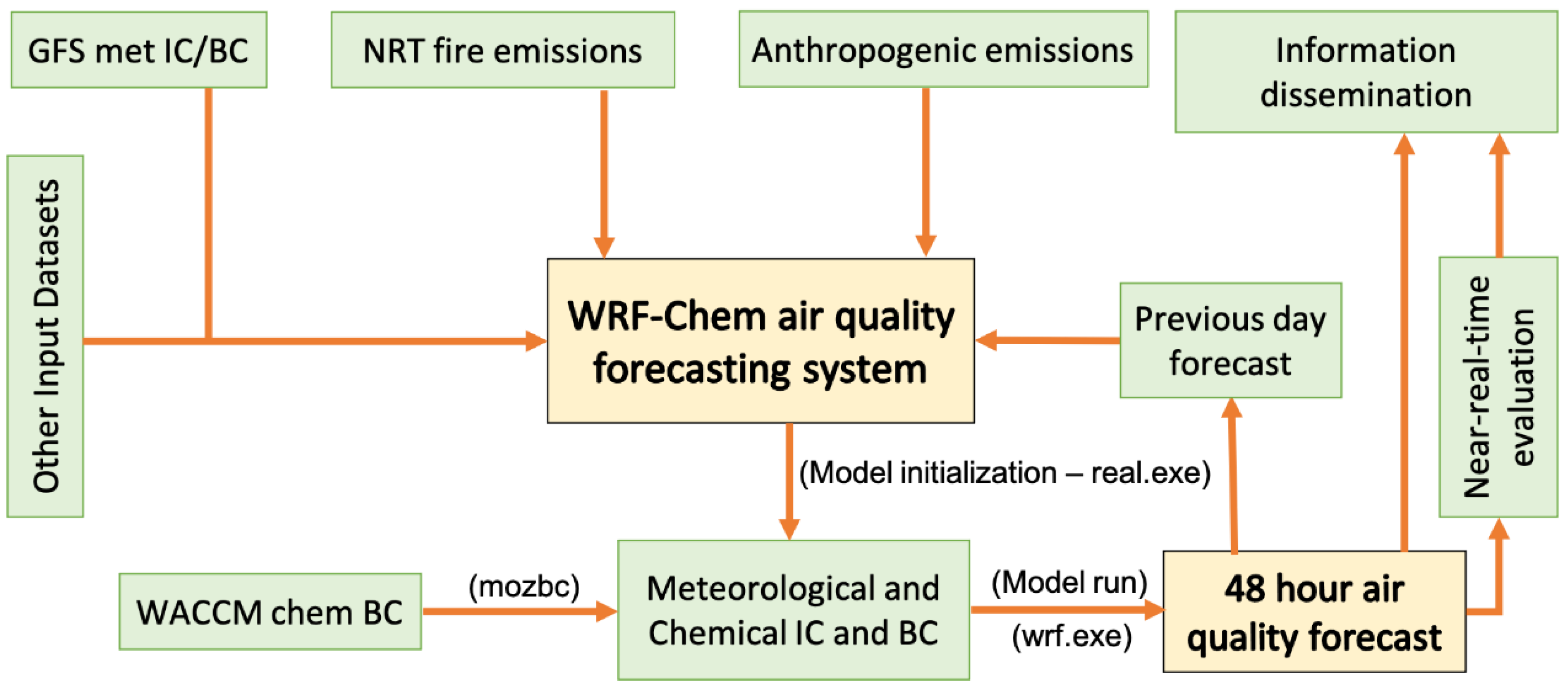
Figure 1. Architecture of the National Center for Atmospheric Research (NCAR) regional air quality forecasting system for the contiguous United States (CONUS). GFS: Global Forecast System; NRT: Near-Real-Time; WACCM: Whole Atmosphere Community Climate Model; IC: Initial conditions; BC: Boundary Conditions.
Atmosphere 12 00302 g001
Figure 2. A snapshot of the information dissemination system. Green, blue, and red arrows point to the drop-down menus where the users can select the chemical species, altitude, and region of their choice. Black arrow points to the button to play/stop animation of the forecast. Figure based on [29].
Atmosphere 12 00302 g002
Figure 3. A snapshot of the information dissemination system showing the access panel with the blue, red, and green arrows pointing to examples of additional evaluation and visualization, Weather Research and Forecasting model coupled with Chemistry (WRF-Chem) ozone vertical profile at a Tropospheric Ozone Lidar Network (TOLNET) site, and comparison with the Tropospheric Monitoring Instrument (TROPOMI) tropospheric column NO2 retrievals. EPA: environmental protection agency. Figure based on [29].
Atmosphere 12 00302 g003
Figure 4. Seasonal variations in hourly and daily observed and model-simulated 2 m temperature in 10 EPA regions during June 2019 to May 2020. Pearson correlation coefficient (r) and mean bias (MB) for each region estimated using paired data for the full year are also shown.
Atmosphere 12 00302 g004
Figure 5. Seasonal variations in hourly and daily observed and model-simulated surface pressure in 10 EPA regions during June 2019 to May 2020. r and MB for each region estimated using paired data for the full year are also shown.
Atmosphere 12 00302 g005
Figure 6. Seasonal variations in hourly and daily observed and model-simulated 2 m relative humidity in 10 EPA regions during June 2019 to May 2020. r and MB for each region estimated using paired data for the full year are also shown.
Atmosphere 12 00302 g006
Figure 7. Seasonal variations in hourly and daily observed and first-day model simulated water vapor mixing ratio (w) in 10 EPA regions during June 2019 to May 2020. Pearson correlation coefficient (r) and mean bias (MB) for each region estimated using paired data for the full year are also shown.
Atmosphere 12 00302 g007
Figure 8. Seasonal variations in hourly and daily observed and model-simulated 10 m wind speed in 10 EPA regions during June 2019 to May 2020. r and MB for each region estimated using paired data for the full year are also shown.
Atmosphere 12 00302 g008
Figure 9. Seasonal variations in hourly and daily observed and model-simulated 10 m wind direction in 10 EPA regions during June 2019 to May 2020. r and MB for each region estimated using paired data for the full year are also shown.
Atmosphere 12 00302 g009
Figure 10. Variations in hourly and daily averaged WRF-Chem forecasted surface PM2.5 mass concentrations against the EPA AirNOW observations in 10 EPA regions from 1 June 2019 to 31 May 2020. r and MB for each region estimated using paired data for the full year are also shown.
Atmosphere 12 00302 g010
Figure 11. Verification of hourly averaged PM2.5 forecasts over 10 EPA regions obtained by averaging PM2.5 values at all Scheme 1 June 2019 to 31 May 2020, is used to calculate average PM2.5 mass concentrations shown here.
Atmosphere 12 00302 g011
Figure 12. Variations in daily averaged WRF-Chem forecasted surface PM2.5 chemical composition in 10 EPA regions from 1 June 2019 to 31 May 2020.
Atmosphere 12 00302 g012
Table 1. Parameterizations used for selected atmospheric processes in the NCAR regional air quality forecasting system.
Atmospheric ProcessParameterization
Cloud MicrophysicsThompson scheme [20]
Short- and Long-wave radiationRapid Radiative Transfer Model for GCMs [21]
Surface LayerEta Similarity [22]
Land Surface modelUnified Noah Land-surface model [23]
Planetary Boundary LayerYonsei University Scheme (YSU) [24]
CumulusGrell-Freitas ensemble scheme [25]
Dry DepositionWesely [26]
Wet DepositionNeu and Prather [27]
PhotolysisTroposphere Ultraviolet Visible (TUV) model
Fire Plume RiseFreitas et al. [11]
Soil NOx emissionsMEGAN v2.0.4 [13,14]
Table 2. Comparison of the range of statistical parameters for the first- and second-day forecasts from 1 June 2019 to 31 May 2020.
rMean BiasRoot Mean Squared Error
Temperature (°C)Day-10.99–1.00−1.52–−0.640.88–1.74
Day-20.99–1.00−1.79–−0.620.84–1.73
Relative humidity (%)Day-10.88–0.960.61–7.433.39–9.21
Day-20.88–0.950.62–7.982.98–8.71
Water vapor mixing ratios (g/kg)Day-10.97–1.00−0.57–−0.010.32–0.68
Day-20.97–0.99−0.71–−0.040.35–0.90
Surface Pressure (hPa)Day-10.63–1.00−7.55–0.010.34–7.61
Day-20.62–0.99−7.67–0.050.61–7.74
Wind Speed (m/s)Day-10.64–0.920.36–1.250.53–1.33
Day-20.32–0.740.25–1.360.49–1.45
Wind Direction (degrees)Day-10.77–0.97−3.43–10.8310.66–25.79
Day-20.76–0.95−5.83–14.9313.02–26.90
PM2.5 (µg m−3) (all sites)Day-10.28–0.67−1.66–0.992.31–3.84
Day-20.29–0.67−1.66–0.992.44–3.77
PM2.5 (µg m−3) (Urban sites)Day-10.24–0.64−1.88–1.062.43–4.06
Day-20.25–0.64−1.85–1.042.57–4.01
PM2.5 (µg m−3) (Suburban sites)Day-10.24–0.67−2.08–1.002.40–3.74
Day-20.25–0.67−2.07–0.992.53–3.66
PM2.5 (µg m−3) (Rural sites)Day-10.24–0.67−2.08–1.002.31–4.02
Day-20.25–0.67−2.07–0.992.33–4.03
PM2.5: fine particulate matter.
Publisher’s Note: MDPI stays neutral with regard to jurisdictional claims in published maps and institutional affiliations.