Estimation of PM_2.5 Concentrations in New York State: Understanding the Influence of Vertical Mixing on Surface PM_2.5 Using Machine Learning

Abstract

In New York State (NYS), episodic high fine particulate matter (PM_2.5) concentrations associated with aerosols originated from the Midwest, Mid-Atlantic, and Pacific Northwest states have been reported. In this study, machine learning techniques, including multiple linear regression (MLR) and artificial neural network (ANN), were used to estimate surface PM_2.5 mass concentrations at air quality monitoring sites in NYS during the summers of 2016–2019. Various predictors were considered, including meteorological, aerosol, and geographic predictors. Vertical predictors, designed as the indicators of vertical mixing and aloft aerosols, were also applied. Overall, the ANN models performed better than the MLR models, and the application of vertical predictors generally improved the accuracy of PM_2.5 estimation of the ANN models. The leave-one-out cross-validation results showed significant cross-site variations and were able to present the different predictor-PM_2.5 correlations at the sites with different PM_2.5 characteristics. In addition, a joint analysis of regression coefficients from the MLR model and variable importance from the ANN model provided insights into the contributions of selected predictors to PM_2.5 concentrations. The improvements in model performance due to aloft aerosols were relatively minor, probably due to the limited cases of aloft aerosols in current datasets.

1. Introduction

Fine particulate matter (PM_2.5) (particulate matter with aerodynamic diameter less than 2.5 µm) is one of the criteria of air pollutants because of its detrimental impacts on human health and the environment [1,2]. Previous studies have reported that the exposure to high PM_2.5 concentrations can increase the risk of respiratory diseases and mortality [3,4]. Many processes can affect ground-level PM_2.5 concentrations, including emissions, removal (e.g., deposition), transport, aerosol physical processes (e.g., nucleation), and atmospheric chemistry [5,6,7,8,9]. These processes are potentially affected by meteorological conditions (e.g., surface temperature and horizontal winds) [10,11,12,13,14]. Yu et al. (2008) [9] used the Eta-Community Multiscale Air Quality (CMAQ) coupled model to estimate the surface PM_2.5 concentrations over the eastern United States (US) during the summer of 2004, and indicated that aerosol physical and chemical processes dominated PM_2.5 concentration. Dawson et al. (2007) [10] analyzed the sensitivities of PM_2.5 concentrations to meteorological variables, and showed that temperature, absolute humidity, wind speed, mixing layer height, and precipitation had the strongest effects on PM_2.5 concentrations. Additionally, atmospheric vertical mixing has been shown to significantly impact PM_2.5 concentrations [7,15,16,17,18,19]. In Zhang et al. (2020) [19], the radar wind profiler measurements showed weak vertical wind shears at a shallower planetary boundary layer (PBL) under polluted conditions, as evidence of weak vertical mixing leading to strong PM_2.5 accumulation in the PBL. They indicated that strong vertical wind shears were associated with strong vertical mixing and often accompanied with low PM_2.5 concentrations. Strong winds above the PBL were also favorable for the transport of aerosols, which could potentially affect surface PM_2.5 concentrations through vertical mixing.

Various approaches have been applied for surface PM_2.5 estimation, including chemistry transport models (CTMs) [9,20,21] and land use regression (LUR) models [22,23]. Statistical approaches based on the relationships between satellite aerosol optical depth (AOD) and surface PM_2.5 concentrations have also been applied [24,25,26]. Recently, machine learning (ML), an application of artificial intelligence (AI), has become an increasingly popular approach for PM_2.5 estimation [27,28,29]. ML also provides insights into contributions of different influencing factors to PM_2.5 concentrations. For instance, Reid et al. (2015) [29] estimated the PM_2.5 concentrations during the Northern California wildfires in 2008. Various predictors were used in ML training, including meteorological variables, such as temperature and humidity, land use variables, such as the distance to the nearest emission source, geographic variables, such as site location and Julian date, satellite AOD measurements, and CTM simulated PM_2.5 concentrations. Meteorological, land use, and geographic variables provided the baseline PM_2.5 estimation. The application of AOD and CTM products further improved model performance by providing the estimation of total-column aerosol loading and prior knowledge of the aerosol physical processes and chemical reactions, respectively. Furthermore, several studies focused on the influence of AOD on PM_2.5 estimation and indicated that AOD could improve the accuracy of PM_2.5 estimation with increased correlation coefficients and decreased model errors [30,31,32,33]. However, Yao et al. (2018) [34] reported an unchanged model performance when using AOD in ML training, probably due to complex terrain, uncertainties of cloud filtering and the presence of aloft aerosols.

In New York State (NYS), the PM_2.5 concentrations have been decreasing continuously over the past decades [35,36,37,38]. Rattigan et al. (2015) [37] analyzed the 2000–2014 observed PM_2.5 concentrations at 16 air quality monitoring sites across the state and reported a downward trend with decreases of 4–7 µg m⁻³ on annual scale. The annual average PM_2.5 concentrations at 15 sites were 9–17 µg m⁻³ and 6–10 µg m⁻³ in 2000 and 2014, respectively, while the annual average PM_2.5 concentration at the Whiteface Mountain site decreased from about 6 µg m⁻³ in 2000 to 4 µg m⁻³ in 2014. In addition, according to the New York State Ambient Air Quality Report for 2019 (https://www.dec.ny.gov/docs/air_pdf/2019airqualreport.pdf), the 2019 PM_2.5 annual averages ranged from 5 to 9 µg m⁻³, except for the Whiteface Mountain site with an annual average around 3 µg m⁻³.

However, episodic high PM_2.5 concentrations across NYS have been reported. During wintertime, the high PM_2.5 concentrations have been attributed to local heating sources and lower mixing layer heights [36,38]. As for summer, the high PM_2.5 concentrations have been attributed to local emissions [39,40], anthropogenic aerosols transported from the Midwest and the Great Lake region [39,40,41,42,43], and long-range transported smoke aerosols from the western US and Canada [44,45,46,47,48]. Climatically, NYS is affected by the prevailing westerlies. Additionally, the Bermuda High locating over the western Atlantic Ocean introduces southerly and southwesterly winds along the east coast in summertime. Under the influences of synoptic flows, air masses could transport aerosols from the polluted areas to NYS. These aerosols could be potentially transported from free troposphere to the surface, resulting in increased PM_2.5 concentrations. In Dutkiewicz et al. (2004) [43], 1-year observations of the concentrations of PM_2.5 sulfate showed that more than 40% of the high sulfate concentrations were associated with westerly flows and around 20–30% were associated with southwesterly flows, reflecting the influences of transported pollutants from the Midwest and Mid-Atlantic states, respectively. The contribution of such transported pollutants was more significant at rural sites, as up to 60% of PM_2.5 sulfate was associated with transported pollutants on annual basis. On the other hand, a statewide event of high PM_2.5 concentrations in August 2018 caused by transported smoke aerosols was investigated in Hung et al. (2020) [45]. Multi-platform measurements and model simulations demonstrated the long-range transport of smoke aerosols from the western states to NYS. These smoke aerosols transported in free troposphere before reaching NYS and descended to around 2 km a.g.l. driven by synoptic downward mixings. The PBL entrainment further brought these aloft aerosols to the surface, resulting in a threefold increase (from 8 to 24 µg m⁻³) in the average PM_2.5 concentrations.

Since transported aerosols make significant contributions to the high PM_2.5 concentrations in NYS, understandings of the relationships between the vertical mixing of these aloft aerosols and surface PM_2.5 concentrations are critical for air quality forecast, monitoring and management. Additionally, studies exploring the roles of vertical mixing in PM_2.5 estimation are needed. In this study, ML techniques were used to estimate the PM_2.5 mass concentrations at air quality monitor sites in NYS during summer seasons (July, August and September, JAS) of 2016–2019. Multiple predictors were applied, including meteorological, aerosol and geographic variables. Predictors associated with vertical mixing and aloft aerosols were also considered. The statistical correlations between selected predictors and PM_2.5 concentrations were investigated. Additionally, to understand the influences of predictors on the PM_2.5 concentration in NYS, the results at monitoring sites with different ambient conditions were discussed.

2. Experiments

2.1. Datasets

The variables used in this study are summarized in

Table 1. List of variables used in this study.

Variable	Source	Level	Spatial Resolution	Temporal Resolution
Target
PM2.5 observation (µg m−3)	EPA AQS 1	Surface		Hourly
Meteorological predictors
Surface pressure (Pa)	HRRR 2	Surface	3 km	3-hourly
Temperature (K)	HRRR	2 m a.g.l.	3 km	3-hourly
Relative humidity (%)	HRRR	2 m a.g.l.	3 km	3-hourly
U-component of horizontal wind (m s−1)	HRRR	10 m a.g.l.	3 km	3-hourly
V-component of horizontal wind (m s−1)	HRRR	10 m a.g.l.	3 km	3-hourly
Planetary boundary layer height (m)	HRRR		3 km	3-hourly
Aerosol predictors
Aerosol optical depth	VIIRS 3	Total column	0.25° × 0.25°	Daily
PM2.5 concentration (µg m−3)	MERRA-2 4	Surface	0.5° × 0.625°	Hourly
Geographic predictors
Latitude	EPA AQS
Longitude	EPA AQS
Altitude (m)	EPA AQS
Vegetation index	VIIRS 5	Surface	0.05° × 0.05°	Monthly
Weekday				Daily
Vertical predictors
Wind shear (s−1)	HRRR	Surface—850 hPa 850—700 hPa 700—500 hPa	3 km	3-hourly
Average vertical velocity (Pa s−1)	HRRR	Surface—500 hPa	3 km	3-hourly
Ratio of AOD change rate to PM change rate	VIIRS		0.25° × 0.25°	Daily
	EPA AQS			Daily

Note: ¹ https://aqs.epa.gov/aqsweb/documents/data_api.html; ² http://home.chpc.utah.edu/~u0553130/Brian_Blaylock/cgi-bin/hrrr_download.cgi; ³ https://www.star.nesdis.noaa.gov/smcd/emb/viirs_aerosol/products_gridded.php; ⁴ https://disc.gsfc.nasa.gov/datasets/M2T1NXAER_5.12.4/summary; ⁵ https://lpdaac.usgs.gov/products/vnp13c2v001/.

and are briefly described in this section. Details can be found in the cited references.

2.1.1. Surface PM_2.5 Observations

The US Environmental Protection Agency (EPA) collects real-time air quality measurements from over 2000 surface monitoring sites nationwide maintained by state or local air quality agencies. In NYS, air quality data are collected and quality controlled by the NYS Department of Environmental Conservation (NYSDEC). In this study, hourly PM_2.5 mass concentrations from 21 monitoring sites across NYS were used (Figure 1;

Table 2. List of PM_2.5 monitor sites in NYS used in this study. Site labels are referred to in Figure 1. Sites using Federal Equivalence Method (FEM) are marked with asterisks *. Sites 1–5, 6–8 and 9–21 are UNY, rural and NYC sites, respectively.

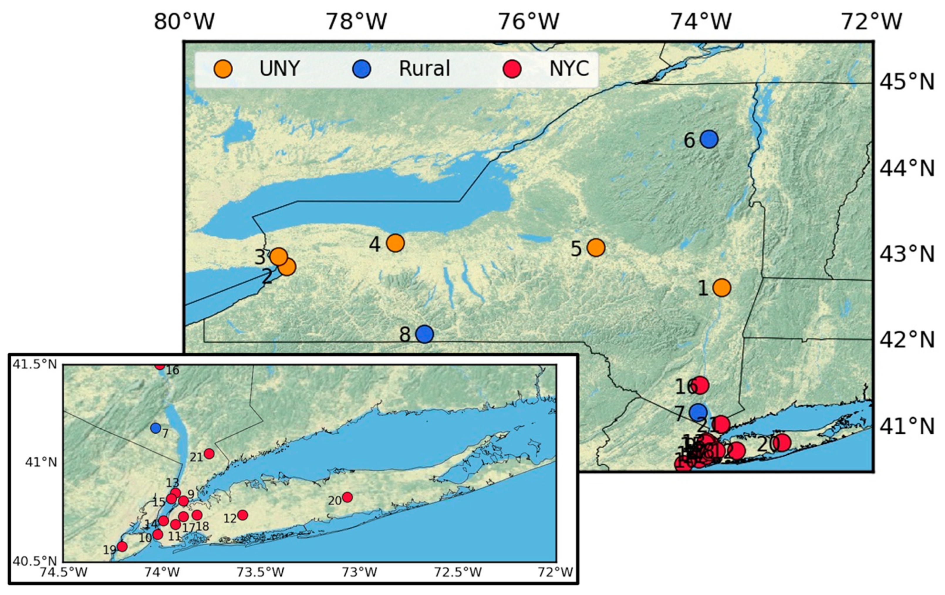
Label	Name	ID Number	Latitude	Longitude	Altitude (m)	Type
1	Albany	360010005	42.64	−73.75	7	UNY
2	Buffalo	360290005	42.88	−78.81	185	UNY
3	Tonawanda II	360291014	43	−78.9	182	UNY
4	Rochester *	360551007	43.15	−77.55	137	UNY
5	Utica	360652001	43.1	−75.22	139	UNY
6	Whiteface Mountain	360310003	44.36	−73.9	599	Rural
7	Rockland County	360870005	41.18	−74.03	140	Rural
8	Pinnacle State Park *	361010003	42.1	−77.21	507	Rural
9	Bronx	360050112	40.81	−73.89	20	NYC
10	PS 314	360470052	40.64	−74.02	26	NYC
11	PS 274	360470118	40.69	−73.93	18	NYC
12	Esienhower Park	360590005	40.74	−73.59	27	NYC
13	IS 143	360610115	40.85	−73.93	0	NYC
14	Division St.	360610134	40.71	−73.99	17	NYC
15	CCNY	360610135	40.82	−73.95	45	NYC
16	Newburgh	360710002	41.5	−74.01	127	NYC
17	Maspeth	360810120	40.73	−73.89	31	NYC
18	Queens *	360810124	40.74	−73.82	25	NYC
19	FKILL	360850111	40.58	−74.2	3	NYC
20	Holtsville	361030009	40.83	−73.06	45	NYC
21	White Plain	361192004	41.05	−73.76	64	NYC

). According to the US EPA and Squizzato et al. (2018) [38], these sites consisted of 18 urban/suburban sites and 3 rural sites. The urban/suburban sites were divided into New York City (NYC) metropolitan sites and upstate NY (UNY) sites based on their locations defined by the US EPA core based statistical areas (CBSA). As a result, in this study, 21 selected sites were categorized into: (1) 5 UNY sites, which is a group of sites in Buffalo, Rochester, and Albany areas, (2) 3 rural sites, and (3) 13 NYC sites, which located in the New York–Newark–Jersey City area. The PM_2.5 concentration measurements at three sites (marked with asterisks in Table 2) are based on the Federal Equivalence Method (FEM), while others are based on the Tapered Element Oscillating Microbalances (TEOM) technology.

2.1.2. Meteorological Predictors

Several meteorological predictors were obtained in this study, including 2 m temperature (T), 2 m relative humidity (RH), surface pressure (PS), planetary boundary layer height (PBLH), and the u and v components of 10 m horizontal winds (U, V). These variables were taken from the analysis fields of the High-Resolution Rapid Refresh (HRRR) [49], which is an atmospheric model developed by the NOAA/Earth System Research Laboratories (ESRL)/Global Systems Laboratory (GSL). HRRR has 3 km horizontal resolution and 51 vertical levels in hybrid coordinates, and provides hourly analysis over the contiguous US (CONUS) and Alaska. Details about HRRR can be found at https://rapidrefresh.noaa.gov/hrrr/ and http://www.nco.ncep.noaa.gov/pmb/products/hrrr/.

2.1.3. Aerosol Predictors

AOD measurements from the Visible Infrared Imaging Radiometer Suite (VIIRS) sensor onboard the Suomi National Polar-orbiting Partnership (S-NPP) satellite, launched in October 2011, were used. VIIRS measures 22 spectrum channels in the range of 412–12,050 nm, including imagery bands, moderate resolution bands (M-bands) and the day–night band. The wide spectral range allows VIIRS to provide multiple land and atmosphere products and the M-bands are mainly used for aerosol retrieval [50]. VIIRS provides daily global coverage with 750 m resolution and only daytime measurements are used for AOD retrieval. In this study, level 3 Environmental Data Record (EDR) daily gridded AOD at 550 nm products were used.

In addition, surface PM_2.5 mass concentrations from the Modern-Era Retrospective analysis for Research and Applications, Version 2 (MERRA-2) [51] were used. MERRA-2 is a global atmospheric reanalysis developed by the National Aeronautics and Space Administration’s (NASA’s) Global Modeling and Assimilation Office (GMAO). MERRA-2 uses the Goddard Earth Observing System, Version 5 (GEOS-5) Atmospheric General Circulation Model (AGCM) coupled with the Goddard Chemistry Aerosol Radiation and Transport (GOCART) model [52]. Aerosol and meteorological observations are jointly assimilated in MERRA-2. MERRA-2 aerosol reanalysis considers aerosol emissions, transport, removal processes, and chemistry. Details can be found in Buchard et al. (2017) [53] and Randles et al. (2017) [54]. A brief comparison between HRRR and MERRA-2 meteorological fields (T, RH, PS, U and V) showed that two models are in good agreement with correlation coefficients higher than 0.7 (Appendix A).

2.1.4. Geographic Predictors

In this study, the monthly enhanced vegetation index (VI) [55,56] products from VIIRS S-NPP were used as terrestrial vegetation estimation. Weekday and geographic information (latitude, longitude and altitude) of selected monitor sites, referred from EPA AQS database, were also used.

2.1.5. Vertical Predictors

To describe the atmospheric vertical mixing, vertical wind shears (VWS) of three layers, including surface—850 hPa (Low-Level; L-VWS), 850–700 hPa (Mid-Level; M-VWS) and 700–500 hPa (High-Level; H-VWS) from HRRR analysis, were used in this study. VWS were defined as the gradients of horizontal winds between the top and bottom model levels. Note that this study only considered the magnitude of VWS, which was computed from the u and v components of VWS. The average vertical velocities of the layer of surface to 500 hPa (W_avg) were also used.

Furthermore, to indicate the presence of aloft aerosols, the daily change rates (R) of AOD and PM_2.5 concentrations at monitor sites were calculated as follows:

$$R_{AOD, d}= \frac{AO{D}_d- AO{D}_{d-1}}{AO{D}_{d-1}}$$

(1)

$$R_{PM2.5, d}= \frac{PM{2.5}_d- PM{2.5}_{d-1}}{PM{2.5}_{d-1}}$$

(2)

where $d$ is date. The day-by-day variation of AP_ratio reflects the change in aerosol vertical distribution. Since AOD and PM_2.5 concentrations present the aerosol loadings in the total-column atmosphere and near the surface, respectively, their daily change rates should be comparable if most of the aerosols are near the surface. $R_{AOD}$ should be higher than $R_{PM2.5}$ if there are aerosols aloft. In contrast, under weak advection with no change in aloft aerosols, $R_{PM2.5}$ could be higher than $R_{AOD}$, since surface PM_2.5 concentration is mainly determined by local emissions. In this study, the ratio of $R_{AOD}$ to $R_{PM2.5}$ (AP_ratio) was used as the indicator of aloft aerosols.

2.1.6. Data Processing

Datasets in the domain of 40.5°N –45.5° N, 72° W–80° W during the summer seasons (JAS) of 2016–2019, 368 days in total, were used. Four data processing steps were taken prior to training. First, spatial linear interpolations were applied for MERRA-2 data, and 3 × 3 grid averages were computed for satellite AOD and VI as the representative at the location of selected air quality sites. Second, the averages of daytime data during 0700–1800 LT (1200–2300 UTC), except for AOD and VI, were calculated. Afterward, days with missing data were removed. The outliers (i.e., values beyond average ±3 standard deviations) of PM_2.5 observation and AOD were also removed to exclude extreme cases (about 1.5% of the data). Lastly, aerosol predictors were transformed to become Gaussian distribution by taking square roots on PM_2.5 observation and AOD and taking a log of MERRA-2 PM_2.5 concentration.

The assumption of independence of predictors, required for ML algorithms, is examined by correlation matrix (Appendix B). While the assumption is not strictly met, the impact on training results may not be significant given only one pair exceeding 0.8. It is worth mentioning that, although some variables may be connected physically (e.g., T and PBLH), the correlations between these variables are relatively weak.

2.2. Model Configuration

Two ML algorithms were used in this study: multiple linear regression (MLR) and artificial neural network (ANN). MLR is a statistical technique which estimates the relationships between several explanatory variables (i.e., predictors) and a response variable (i.e., target) by fitting a linear regression to the ground truth (PM_2.5 observations in this study). It generates a linear regression of given variables, including the coefficients for predictors and intercept. In this study, the Python Scikit-Learn package [57] was used to build the MLR models.

An artificial neural network (ANN), one of the most popular ML algorithms, is effective for handling complex nonlinear problems, particularly in classification and prediction [58,59]. An ANN model consists of a set of layers, including the input layer, multiple hidden layers, and the output layer. There is no specific rule to decide how many hidden layers an ANN model should have but one hidden layer with abundant neurons usually provides good results [58]. In addition, previous studies showed that ANN models performed better with the number of neurons in a range of (2√n + φ,2n + 1), where n and φ are the numbers of predictors and targets, respectively [60]. In this study, the Python Keras and Tensorflow packages [61] were used. Back-propagation models with one hidden layer obtaining 20 neurons were applied. The maximum number of iterations was set to 1000 and an EarlyStopping function (https://keras.io/api/callbacks/early_stopping/) was used to avoid overfitting. Variables were randomly split into the training set (80%) and validation set (20%) in the training process, and an additional testing set, which will be described in the following section, was applied for model evaluation.

To investigate the influence of vertical mixing and aloft aerosols on surface PM_2.5 concentration, two sets of predictors were applied. Set 1 contained meteorological, aerosol, and geographic predictors, while set 2 contained the same predictors as set 1 but also included vertical predictors. Therefore, four models were applied in this study:

• MLR model with set 1 predictors (MLR-1);
• MLR model and set 2 predictors (MLR-2);
• ANN model with set 1 predictors (ANN-1);
• ANN model with set 2 predictors (ANN-2).

2.3. Statistical Analysis

In this study, leave-one-out cross validation (LOOCV) [62] was used for model performance evaluation. All four models were trained on data from all monitor sites but one and were tested on the leave-out site. This process was repeated until all 21 sites served as the test site once. Therefore, LOOCV ensured independent evaluation of the trained model via comparison of the predicted and observed values at the locations that did not participate in the training. The involvement of spatial dependence allowed LOOCV to provide more reliable estimations of model performance [63]. Three statistical scores were used for model evaluation, including mean bias (MB), coefficient of determination (R²), and root mean square error (RMSE). These scores were calculated as follows:

$$MB= \frac{1}{n} {\displaystyle \sum }_i^n{Y}_i- X_i$$

(3)

$$R^2= {\left(\frac{{{\displaystyle \sum }}_i^n\left(Y_i- \overline{Y}\right){{\displaystyle \sum }}_i^n\left(X_i- \overline{X}\right)}{\sqrt{{{\displaystyle \sum }}_i^n{\left(Y_i- \overline{Y}\right)}^2}\sqrt{{{\displaystyle \sum }}_i^n{\left(X_i- \overline{X}\right)}^2}}\right)}^2$$

(4)

$$RMSE= \sqrt{\frac{1}{n} {\displaystyle \sum }_i^n{\left(Y_i- X_i\right)}^2}$$

(5)

where $n$ is number of data points, $X$ is observation, $Y$ is prediction, and $\overline{X}$ and $\overline{Y}$ are the averages of observation and prediction, respectively. The scores at test sites were then averaged as the estimated model errors. Although LOOCV is beneficial for estimating the spatial dependence within trained models, the imbalanced site distribution in NYS (over 60% of the sites are in NYC region) may introduce representativeness issues in the model performance.

To understand the relationships between predictors and PM_2.5 concentrations, the regression coefficients from the MLR models and permutation importance estimated from the ANN models were analyzed. The values of regression coefficients explained the change in target when applying one unit of change in predictors, and the signs explained the direction of such a change. Permutation importance is an approach for ranking variable importance [64,65]. The goal of this approach is to estimate how model performance changes when breaking the correlations between predictors and target. This is done by randomly shuffling one predictor in the test data, and comparing the statistical scores of the shuffled model and unshuffled model. Larger percentage errors indicate higher importance. This process is repeated until all predictors have been shuffled once. In this study, the percentage error of the RMSE values of two models was regarded as the estimation of variable importance and is calculated as follows.

$$Variable importance= \frac{RMS{E}_{shuffled}- RMS{E}_{unshuffled}}{RMS{E}_{unshuffled}} \times 100\%$$

(6)

3. Results and Discussion

3.1. Model Performance

Figure 2 illustrates the LOOCV testing results at selected monitoring sites of the four models. The averages of statistical scores are shown in

Table 3. Averaged statistical scores of four models at 21 selected sites.

Model	Bias (µg m−3)	R-Squared	RMSE (µg m−3)
MLR-1	0.03 ± 1.14	0.51 ± 0.06	2.96 ± 0.26
MLR-2	0.06 ± 1.31	0.52 ± 0.06	3.01 ± 0.39
ANN-1	−0.63 ± 0.99	0.65 ± 0.09	2.59 ± 0.45
ANN-2	−0.29 ± 0.88	0.67 ± 0.10	2.42 ± 0.37

, and the statistical scores at individual sites are shown in Appendix C and Appendix D. Overall, the ANN models performed better than the MLR models with higher R² and lower RMSE, and the ANN models showed larger cross-site variations compared to the MLR models. The absolute values of averaged MB of the ANN models (0.63 and 0.29 µg m⁻³) were higher than the MLR models (0.03 and 0.06 µg m⁻³). However, the MBs at individual sites of the four models had a similar range of 2 µg m⁻³, except for the MLR-2 model which had a wider range of ±3 µg m⁻³. In addition, the near-zero averaged MBs compared to RMSEs indicated that there were negative and positive biases and those non-systemic biases cancelled out in averaging for the MLR and ANN models.

For the MLR models, the application of vertical predictors introduced a neutral impact to the model performance since the differences of averaged statistical scores between MLR-1 and MLR-2 were relatively minor. The RMSE at two rural sites (sites 6 and 8) even increased by 0.5–1 µg m⁻³ when applying vertical predictors (Figure 2a), resulting in a slightly increased averaged RMSE (Table 3). In contrast, the improvement due to vertical predictors was more significant for the ANN models (Figure 2b). The application of vertical predictors slightly increased the averaged MB for the MLR models (from 0.03 to 0.06 µg m⁻³), while it reduced the averaged MB for ANN models (from −0.63 to −0.29 µg m⁻³) (Table 3). Additionally, the range of RMSE changed from (1.92 to 3.89 µg m⁻³) for the ANN-1 model to (1.64 to 3.32 µg m⁻³) for the ANN-2 model (Appendix D), showing a general improvement in model performance. It is worth mentioning that the MB and RMSE at sites 6 and 8 decreased by around 2 µg m^-3, showing contrary results to the MLR models.

3.2. The Site-Variations of Model Performance

The model performance with the influence of vertical predictors on PM_2.5 prediction at different category of sites were investigated. Figure 3 demonstrates the differences in statistical scores between the models using set 1 and set 2 predictors at selected air quality sites.

Table 4. Averaged statistical scores of four models at rural, NYC and UNY sites.

Model	Bias (µg m−3)	R-Squared	RMSE (µg m−3)
Rural sites
MLR-1	−0.15 ± 2.04	0.55 ± 0.01	3.11 ± 0.20
MLR-2	0.07 ± 2.67	0.54 ± 0.02	3.53 ± 0.54
ANN-1	−2.10 ± 1.00	0.61 ± 0.04	3.25 ± 0.51
ANN-2	−1.02 ± 0.70	0.64 ± 0.06	2.40 ± 0.12
NYC sites
MLR-1	0.09 ± 0.80	0.53 ± 0.05	2.85 ± 0.16
MLR-2	0.10 ± 0.80	0.54 ± 0.05	2.84 ± 0.15
ANN-1	−0.42 ± 0.76	0.68 ± 0.09	2.42 ± 0.33
ANN-2	−0.19 ± 0.89	0.71 ± 0.09	2.31 ± 0.38
UNY sites
MLR-1	−0.04 ± 1.09	0.45 ± 0.04	3.13 ± 0.35
MLR-2	−0.05 ± 1.12	0.44 ± 0.04	3.15 ± 0.36
ANN-1	−0.31 ± 0.70	0.59 ± 0.05	2.66 ± 0.29
ANN-2	−0.13 ± 0.76	0.58 ± 0.05	2.71 ± 0.24

shows the averages of statistic scores of each category of sites. The statistical scores at each site are listed in Appendix C and Appendix D. Overall, the results showed variations in model performance across the state, reflecting the different air quality characteristics.

For rural sites, the RMSEs of the MLR-2 model at site 6 and 8 increased from 3.22 and 3.29 µg m⁻³ to 4.13 and 3.65 µg m⁻³, respectively, compared to the MLR-1 model. The MBs at the two sites also increased, showing that the model performance degraded when applying vertical predictors to the MLR model. In contrast, the performance of the ANN models at three rural sites showed significant improvement with increased R² and decreased MB and RMSE. The contrasting performance of the MLR and ANN models could be attributed to the complexity and nonlinearity of the influences of vertical predictors on PM_2.5 concentrations, which could not be learned by the MLR models. Additional predictors could even reduce the significance of the correlations between other predictors and PM_2.5 concentrations in the MLR models. It is worth noting that the testing results at site 6 (Whiteface Mountain site, the fifth highest mountain in NYS) showed the most significant differences after applying vertical predictors for both the MLR and ANN models. This is probably because the PM_2.5 concentrations at Whiteface Mountain are mainly affected by meteorological conditions and transported aerosols [43].

For NYC sites, both the averaged values (Table 4) and testing results at individual site (Appendix C) showed comparable statistical scores for two MLR models. Although the performance of the ANN models showed neutral to positive impacts when applying vertical predictors, the differences in statistical scores were less significant than those at rural sites. This is probably because the air quality of NYC sites is influenced by local anthropogenic emissions and photochemical reactions near the surface, and thus the influence of vertical mixing is limited.

For UNY sites, the statistical scores of the MLR models were comparable, showing limited influence of vertical predictors. As for the ANN models, model performance showed degradation with increased MB at most of the sites after applying vertical predictors (Appendix D). The reductions in RMSE at three sites were relatively minor compared to the increases at two sites, resulting in an increased average value. This may be due to the spatial variability among UNY sites. Unlike NYC sites, UNY sites are a group of urban/suburban sites across the state influenced by different local emissions. The influences of vertical mixing varied among these sites, leading to the degraded testing results on average.

Additionally, to better understand the influence of vertical predictors on PM_2.5 prediction at each category of sites, the testing results at three sites with the lowest RMSEs were analyzed. The PS 314, Rockland County, and Rochester sites were selected as the representatives of NYC, rural and UNY sites, respectively. Additionally, since vertical predictors showed limited contributions in the MLR models in previous discussions, only the results from the ANN models were discussed. Figure 4 illustrates the scatter plots between observed and predicted PM_2.5 concentrations from the ANN models and the corresponding data plots at selected sites. For PS 314 site (Figure 4a), data plots showed that the ANN-2 model had better performance in predicting spikes with smaller differences between observations and predictions, compared to the ANN-1 model. Although the differences were small, the positive effects of vertical predictors on PM_2.5 concentrations at NYC sites were not neglectable. Similarly, the testing results of the ANN models at Rockland County site (Figure 4b) showed that the ANN-2 model had better capability of predicting spikes. Although the ANN-2 model still showed outliers in the scatter plot, it provided more accurate estimations with higher R² and lower RMSE. On the other hand, the testing results from two ANN models at Rochester site (Figure 4c) were comparable, showing a limited influence of vertical mixing.

3.3. The Contributions of Predictors to Surface PM_2.5 Concentrations

In this section, the regression coefficients generated by the MLR models and variable importance estimated from the ANN models were investigated. Figure 5, Figure 6 and Figure 7 show the signs of regression coefficients and variable importance at the PS 314, Rochester, and Rockland County sites, respectively. Note that Lat, Lon, and Alt are fixed values at each site, thus shuffling them did not affect the results. The values of regression coefficients are listed in Appendix E.

For all sites, MERRA-2 PM_2.5 concentration and T showed the highest importance. The positive regression coefficients of MERRA-2 PM_2.5 concentration were related to the positive effects of aerosol removal processes and chemical reactions on PM_2.5 concentrations. The positive coefficients of T were consistent with previous studies [10,11], which showed warm condition was conductive for photochemical formation of secondary aerosols. Thus, the high importance of two predictors collectively indicated that aerosol removal processes and chemical reactions played a dominant role in PM_2.5 concentration during the daytime. Furthermore, the high importance of PBLH at the PS 314 and Rochester sites indicated the significant dispersion effect in the PBL. During the daytime, radiative heating on the surface led to a sharp increase in PBLH, resulting in decreasing the PM_2.5 concentration due to stronger dispersion. The weekday also showed significant importance at all sites. The negative coefficients between weekday and PM_2.5 concentrations may be associated with the anthropogenic emissions from industries and traffic during weekdays.

Additionally, surface wind fields, U and V, and VWSs showed moderate importance. The positive coefficients of U and V indicated the positive effects of westerly (positive U) and southerly (positive V) winds, respectively. This was consistent with previous studies, which showed that high PM_2.5 concentrations were associated with transported aerosols driven by westerly and southwesterly flows [41,42]. Moreover, the negative coefficients of M-VWS and L-VWS showed that weak air mass exchanges above the PBL and stable conditions in the PBL potentially led to high PM_2.5 concentrations, respectively. These results could be associated with the frontal systems caused by the westerly mid-latitude cyclones, which are common during summer in the Northeast US [42,66]. Additionally, the strong VWS at higher troposphere could be beneficial for the downward transport of long-range transported aerosols (e.g., smoke aerosols), resulting in the positive correlation between H-VWS and PM_2.5 concentrations.

At the PS 314 site (Figure 5), the VWS at three levels played a relatively weak role in PM_2.5 concentrations compared to the surface conditions. This was consistent with previous discussion, which mentioned that the influence of local ambient conditions on PM_2.5 concentrations were more significant than vertical mixing at NYC sites. In contrast, M-VWS and L-VWS at the Rochester site (Figure 6) showed comparable importance with surface winds and RH, indicating a similar, even stronger, influence of vertical mixing than surface ambient conditions. Similar phenomenon was also found at Rockland County site (Figure 7), with higher importance of M-VWS and H-VWS than surface winds, RH and PBLH. In addition, the low importance of PBLH and L-VWS at the Rockland County site may indicate a weak PBL-PM_2.5 correlation, since the PM_2.5 concentrations at rural sites are relatively low and not dominated by local emissions.

The positive correlation between AOD and PM_2.5 concentrations was expected. Since AOD is an indicator of total-column aerosol loadings, higher AOD represents higher PM_2.5 concentration particularly when most of the columnar aerosol loading is present in the PBL. According to previous studies, AOD showed significant impacts on PM_2.5 concentrations with high variable importance [32]. However, in this study, AOD had moderate importance and relatively weak influence compared to most of the other predictors. This could be due to the application of MERRA-2 PM_2.5 concentration. MERRA-2 is an aerosol reanalysis, which consists of both model simulations and observation assimilation. Therefore, MERRA-2 PM_2.5 concentration already includes AOD information from the assimilated AOD measurements. The AOD assimilation in MERRA-2 could contribute to the high importance of MERRA-2 PM_2.5 concentration. Since aerosol removal processes and chemical reactions were dominant during the daytime, MERRA-2 PM_2.5 concentration showed higher importance than AOD alone. The model results without MERRA-2 PM_2.5 concentration (not shown) also indicated the significant contributions of aerosol photochemical reactions with the highest importance of T.

Based on the definition, high AP_ratio reflects the presence of aloft aerosol layers and positive W_avg represents the atmospheric downward mixing. With strong downward mixings, aloft aerosols could descend to the surface, resulting in increasing the surface PM_2.5 concentrations. The positive coefficients at all sites indicated the positive effects of aloft aerosols on PM_2.5 concentrations. However, the low importance of the two predictors showed that the influence of aloft aerosols was relatively minor. It was probably because of the limited cases of the presence of high PM_2.5 concentrations and aloft aerosols, and the capability of AP_ratio in representing aloft aerosols. In addition, the low importance of PS could be due to its dependence on Alt. Atmospheric pressure provides information about circulation patterns, synoptic weather systems, and atmospheric stability conditions. Since PS decreases with height, such relation may dilute the connection between PS and meteorology, and the correlation between PS and PM_2.5 concentrations, especially for UNY and rural sites with a wide range of Alt values.

4. Conclusions

In NYS, episodic high PM_2.5 concentrations due to transported aerosols have been reported in summer. Driven by synoptic downward mixing and PBL entrainment, pollutants potentially transport from free troposphere into the PBL and affect PM_2.5 concentrations near the surface. In light of the contributions of transported aerosols to high PM_2.5 concentrations in NYS, understandings of the relationships between the vertical mixing of aloft aerosols and PM_2.5 concentrations are important. This study investigated the influences of various factors on the PM_2.5 concentrations in NYS by analyzing the testing results of multiple linear regression (MLR) and artificial neural network (ANN) models trained with two sets of predictors. Overall, the ANN models performed better than MLR models. Additionally, for the ANN models, the predictors of vertical mixing and aloft aerosols improved the MB, R² and RMSE by 0.34, 0.02 and 0.17 µg m⁻³, respectively, on average. Although RMSEs around 3 µg m⁻³ were relatively high for NYS, as the RMSEs were one-third and/or close to the annual PM_2.5 average concentrations of 2019, the improvements in model performance were non-negligible. The leave-one-out cross-validation results showed significant site-variations and were able to differentiate predictor-PM_2.5 correlations at sites with different air quality characteristics. The model improvement due to vertical mixing and aloft aerosols was more significant at rural sites, where the PM_2.5 concentrations are mainly affected by meteorology and transported aerosols. The changes in model performance at UNY sites varied among sites, probably due to the spatial variability within a wide region of UNY. In addition, a joint analysis of regression coefficients and variable importance provided insights into the contributions of selected predictors to PM_2.5 concentration. The aerosol removal process and chemical reactions showed the highest importance at three categories of sites (UNY, NYC and rural), and the contribution of vertical mixing was more significant at UNY and rural sites. However, the influence of aloft aerosols was limited in the current results. Identifying the cases of high PM_2.5 concentrations associated with transported aerosols prior to training may provide more significant results and better understanding of the influence of aloft aerosols.

References

- Pope, I.C.; Burnett, R.T.; Thun, M.J.; Calle, E.E.; Krewski, D.; Ito, K.; Thurston, G.D. Lung cancer, cardiopulmonary mortality, and long-term exposure to fine particulate air pollution. J. Am. Med. Assoc. 2002, 287, 1132–1141. [Google Scholar] [CrossRef] [PubMed]
- Pope, C.A.; Burnett, R.T., III; Thurston, G.D.; Thun, M.J.; Calle, E.E.; Krewski, D.; Godleski, J.J. Cardiovascular Mortality and Long-Term Exposure to Particulate Air Pollution: Epidemiological Evidence of General Pathophysiological Pathways of Disease. Circulation 2004, 1, 71–77. [Google Scholar] [CrossRef] [PubMed]
- Apte, J.S.; Marshall, J.D.; Cohen, A.J.; Brauer, M. Addressing Global Mortality from Ambient PM2.5. Environ. Sci. Technol. 2015, 49, 8057–8066. [Google Scholar] [CrossRef] [PubMed]
- Franklin, M.; Zeka, A.; Schwartz, J. Association between PM2.5 and all-cause and specific-cause mortality in 27 US communities. J. Expo. Sci. Environ. Epidemiol. 2007, 17, 279–287. [Google Scholar] [CrossRef]
- Behera, S.N.; Sharma, M. Reconstructing Primary and Secondary Components of PM2.5 Composition for an Urban Atmosphere. Aerosol Sci. Technol. 2010, 44, 983–992. [Google Scholar] [CrossRef]
- Edney, E.O.; Kleindienst, T.E.; Jaoui, M.; Lewandowski, M.; Offenberg, J.H.; Wang, W.; Claeys, M. Formation of 2-methyltetrols and 2-methylglyceric acid in secondary organic aerosol from laboratory irradiated isoprene/NOX/SO2/air mixtures and their detection in ambient PM2.5 samples collected in the eastern United States. Atmos. Environ. 2005, 39, 5281–5289. [Google Scholar] [CrossRef]
- Lonati, G.; Ozgen, S.; Giugliano, M. Primary and secondary carbonaceous species in PM2.5 samples in Milan (Italy). Atmos. Environ. 2007, 41, 4599–4610. [Google Scholar] [CrossRef]
- Wang, Y.; Zhuang, G.; Tang, A.; Yuan, H.; Sun, Y.; Chen, S.; Zheng, A. The ion chemistry and the source of PM2.5 aerosol in Beijing. Atmos. Environ. 2005, 39, 3771–3784. [Google Scholar] [CrossRef]
- Yu, S.; Mathur, R.; Schere, K.; Kang, D.; Pleim, J.; Young, J.; Tong, D.; Pouliot, G.; McKeen, S.A.; Rao, S.T. Evaluation of real-time PM2.5 forecasts and process analysis for PM2.5 formation over the eastern United States using the Eta-CMAQ forecast model during the 2004 ICARTT study. J. Geophys. Res. 2008, 113, D06204. [Google Scholar] [CrossRef]
- Dawson, J.P.; Adams, P.J.; Pandis, S.N. Sensitivity of PM2.5 to climate in the Eastern US: A modeling case study. Atmos. Chem. Phys. 2007, 7, 4295–4309. [Google Scholar] [CrossRef]
- Tai, A.P.K.; Mickley, L.J.; Jacob, D.J. Correlations between fine particulate matter (PM2.5) and meteorological variables in the United States: Implications for the sensitivity of PM2.5 to climate change. Atmos. Environ. 2010, 44, 3976–3984. [Google Scholar] [CrossRef]
- Tran, H.N.Q.; Mölders, N. Investigations on meteorological conditions for elevated PM2.5 in Fairbanks, Alaska. Atmos. Res. 2011, 99, 39–49. [Google Scholar] [CrossRef]
- Wang, J.; Ogawa, S. Effects of Meteorological Conditions on PM2.5 Concentrations in Nagasaki, Japan. Int. J. Environ. Res. Public Health 2015, 12, 9089–9101. [Google Scholar] [CrossRef] [PubMed]
- Zhang, Z.; Zhang, X.; Gong, D.; Quan, W.; Zhao, X.; Ma, Z.; Kim, S.-J. Evolution of surface O3 and PM2.5 concentrations and their relationships with meteorological conditions over the last decade in Beijing. Atmos. Environ. 2015, 108, 67–75. [Google Scholar] [CrossRef]
- Chen, Y.; An, J.; Wang, X.; Sun, Y.; Wang, Z.; Duan, J. Observation of wind shear during evening transition and an estimation of submicron aerosol concentrations in Beijing using a Doppler wind lidar. J. Meteor. Res. 2017, 31, 350–362. [Google Scholar] [CrossRef]
- Li, Z.; Guo, J.; Ding, A.; Liao, H.; Liu, J.; Sun, Y.; Wang, T.; Xue, H.; Zhang, H.; Zhu, B. Aerosol and boundary-layer interactions and impact on air quality. Nat. Sci. Rev. 2017, 4, 810–833. [Google Scholar] [CrossRef]
- Yang, Y.; Yim, S.H.L.; Haywood, J.; Osborne, M.; Chan, J.C.S.; Zeng, Z.; Cheng, J.C.H. Characteristics of heavy particulate matter pollution events over Hong Kong and their relationships with vertical wind profiles using high-time-resolution Doppler lidar measurements. J. Geophys. Res. Atmos. 2019, 124, 9609–9623. [Google Scholar] [CrossRef]
- Zhang, J.; Rao, S.T. The Role of Vertical Mixing in the Temporal Evolution of Ground-Level Ozone Concentrations. J. Appl. Meteor. 1999, 38, 1674–1691. [Google Scholar] [CrossRef]
- Zhang, Y.; Guo, J.; Yang, Y.; Wang, Y.; Yim, S.H.L. Vertical Wind Shear Modulates Particulate Matter Pollutions: A Perspective from Radar Wind Profiler Observations in Beijing, China. Remote Sens. 2020, 12, 546. [Google Scholar] [CrossRef]
- Hu, J.; Chen, J.; Ying, Q.; Zhang, H. One-year simulation of ozone and particulate matter in China using WRF/CMAQ modeling system. Atmos. Chem. Phys. 2016, 16, 10333–10350. [Google Scholar] [CrossRef]
- Saide, P.E.; Carmichael, G.R.; Spak, S.N.; Gallardo, L.; Osses, A.E.; Mena-Carrasco, M.A.; Pagowski, M. Forecasting urban PM10 and PM2.5 pollution episodes in very stable nocturnal conditions and complex terrain using WRF–Chem CO tracer model. Atmos. Environ. 2011, 45, 2769–2780. [Google Scholar] [CrossRef]
- Eeftens, M.; Beelen, R.; de Hoogh, K.; Bellander, T.; Cesaroni, G.; Cirach, M.; Declercq, C.; Dėdelė, A.; Dons, E.; De Nazelle, A.; et al. Development of Land Use Regression Models for PM2.5, PM2.5 Absorbance, PM10 and PMcoarse in 20 European Study Areas; Results of the ESCAPE Project. Environ. Sci. Technol. 2012, 46, 11195–11205. [Google Scholar] [CrossRef] [PubMed]
- Hoek, G.; Beelen, R.; de Hoogh, K.; Vienneau, D.; Gulliver, J.; Fischer, P.; Briggs, D. A review of land-use regression models to assess spatial variation of outdoor air pollution. Atmos. Environ. 2008, 42, 7561–7578. [Google Scholar] [CrossRef]
- Chu, Y.; Liu, Y.; Li, X.; Liu, Z.; Lu, H.; Lu, Y.; Mao, Z.; Chen, X.; Li, N.; Ren, M.; et al. A Review on Predicting Ground PM2.5 Concentration Using Satellite Aerosol Optical Depth. Atmosphere 2016, 7, 129. [Google Scholar] [CrossRef]
- Liu, Y.; Sarnat, J.A.; Kilaru, V.; Jacob, D.J.; Koutrakis, P. Estimating Ground-Level PM2.5 in the Eastern United States Using Satellite Remote Sensing. Environ. Sci. Technol. 2005, 39, 3269–3278. [Google Scholar] [CrossRef] [PubMed]
- Van Donkelaar, A.; Martin, R.V.; Spurr, R.J.D.; Burnett, R.T. High-Resolution Satellite-Derived PM2.5 from Optimal Estimation and Geographically Weighted Regression over North America. Environ. Sci. Technol. 2015, 49, 10482–10491. [Google Scholar] [CrossRef]
- Gupta, P.; Christopher, S.A. Particulate matter air quality assessment using integrated surface, satellite, and meteorological products: Multiple regression approach. J. Geophys. Res. 2009, 114, D14205. [Google Scholar] [CrossRef]
- Gupta, P.; Christopher, S.A. Particulate matter air quality assessment using integrated surface, satellite, and meteorological products: 2. A neural network approach. J. Geophys. Res. 2009, 114, D20205. [Google Scholar] [CrossRef]
- Reid, C.E.; Jerrett, M.; Petersen, M.L.; Pfister, G.G.; Morefield, P.E.; Tager, I.B.; Raffuse, S.M.; Balmes, J.R. Spatiotemporal Prediction of Fine Particulate Matter During the 2008 Northern California Wildfires Using Machine Learning. Environ. Sci. Technol. 2015, 49, 3887–3896. [Google Scholar] [CrossRef]
- Engel-Cox, J.A.; Holloman, C.H.; Coutant, B.W.; Hoff, R.M. Qualitative and quantitative evaluation of MODIS satellite sensor data for regional and urban scale air quality. Atmos. Environ. 2004, 38, 2495–2509. [Google Scholar] [CrossRef]
- Weber, S.A.; Engel-Cox, J.A.; Hoff, R.M.; Prados, A.I.; Zhang, H. An improved method for estimating surface fine particle concentrations using seasonally adjusted satellite aerosol optical depth. J. Air Waste Manag. Assoc. 2010, 60, 574–585. [Google Scholar] [CrossRef] [PubMed]
- Xu, Y.; Ho, H.C.; Wong, M.S.; Deng, C.; Shi, Y.; Chan, T.-C.; Knudby, A. Evaluation of machine learning techniques with multiple remote sensing datasets in estimating monthly concentrations of ground-level PM2.5. Environ. Pollut. 2018, 242, 1417–1426. [Google Scholar] [CrossRef] [PubMed]
- Xue, T.; Zheng, Y.; Tong, D.; Zheng, B.; Li, X.; Zhu, T.; Zhang, Q. Spatiotemporal continuous estimates of PM2.5 concentrations in China, 2000–2016: A machine learning method with inputs from satellites, chemical transport model, and ground observations. Environ. Int. 2019, 123, 345–357. [Google Scholar] [CrossRef] [PubMed]
- Yao, J.; Brauer, M.; Raffuse, S.; Henderson, S.B. Machine Learning Approach to Estimate Hourly Exposure to Fine Particulate Matter for Urban, Rural, and Remote Populations during Wildfire Seasons. Environ. Sci. Technol. 2018, 52, 13239–13249. [Google Scholar] [CrossRef] [PubMed]
- Emami, F.; Masiol, M.; Hopke, P.K. Air pollution at Rochester, NY: Long-term trends and multivariate analysis of upwind SO2 source impacts. Sci. Total Environ. 2018, 612, 1506–1515. [Google Scholar] [CrossRef] [PubMed]
- Rattigan, O.V.; Felton, H.D.; Bae, M.-S.; Schwab, J.J.; Demerjian, K.L. Multi-year hourly PM2.5 carbon measurements in New York: Diurnal, day of week and seasonal patterns. Atmos. Environ. 2010, 44, 2043–2053. [Google Scholar] [CrossRef]
- Rattigan, O.V.; Civerolo, K.L.; Felton, H.D.; Schwab, J.J.; Demerjian, K.L. Long Term Trends in New York: PM2.5 Mass and Particle Components. Aerosol Air Qual. Res. 2015, 16, 191–1203. [Google Scholar] [CrossRef]
- Squizzato, S.; Masiol, M.; Rich, D.Q.; Hopke, P.K. PM2.5 and gaseous pollutants in New York state during 2005–2016: Spatial variability, temporal trends, and economic influences. Atmos. Environ. 2018, 183, 209–224. [Google Scholar] [CrossRef]
- Bari, A.; Dutkiewicz, V.A.; Judd, C.D.; Wilson, L.R.; Luttinger, D.; Husain, L. Regional sources of particulate sulfate, SO2, PM2.5, HCL, HNO3, HONO and NH3 in New York, NY. Atmos. Environ. 2003, 37, 2837–2844. [Google Scholar] [CrossRef]
- Qin, Y.; Kim, E.; Hopke, P.K. The concentrations and sources of PM2.5 in metropolitan New York City. Atmos. Environ. 2006, 40, 312–332. [Google Scholar] [CrossRef]
- DeGaetano, A.T.; Doherty, O.M. Temporal, spatial and meteorological variations in hourly PM2.5 concentration extremes in New York City. Atmos. Environ. 2004, 38, 1547–1558. [Google Scholar] [CrossRef]
- Dutkiewicz, V.A.; Das, M.; Husain, L. The relationship between regional SO2 emissions and downwind aerosol sulfate concentrations in the Northeastern US. Atmos. Environ. 2000, 34, 1821–1832. [Google Scholar] [CrossRef]
- Dutkiewicz, V.A.; Qureshi, S.; Khan, A.R.; Ferraro, V.; Schwab, J.; Demerjian, K.; Husain, L. Sources of fine particulate sulfate in New York. Atmos. Environ. 2004, 38, 3179–3189. [Google Scholar] [CrossRef]
- Dutkiewicz, V.A.; Husain, L.; Roychowdhury, U.K.; Demerjian, K.L. Impact of Canadian wildfire smoke on air quality at two rural sites in NY State. Atmos. Environ. 2011, 45, 2028–2033. [Google Scholar] [CrossRef]
- Hung, W.-T.; Lu, C.-H.S.; Shrestha, B.; Lin, H.-C.; Lin, C.-A.; Grohan, D.; Hong, J.; Ahmadov, R.; James, E.; Joseph, E. The impacts of transported wildfire smoke aerosols on surface air quality in New York State: A case study in summer 2018. Atmos. Environ. 2020, 227, 117415. [Google Scholar] [CrossRef]
- Roger, H.M.; Ditto, J.C.; Gentner, D.R. Evidence for impacts on surface-level air quality in the northeastern US from long-distance transport of smoke from North American fires during the Long Island Sound Tropospheric Ozone Study (LISTOS) 2018. Atmos. Chem. Phys. 2020, 20, 671–682. [Google Scholar] [CrossRef]
- Wu, Y.; Arapi, A.; Huang, J.; Gross, B.; Moshary, F. Intra-continental wildfire smoke transport and impact on local air quality observed by ground-based and satellite remote sensing in New York City. Atmos. Environ. 2018, 187, 266–281. [Google Scholar] [CrossRef]
- Zu, K.; Tao, G.; Long, K.; Goodman, J.; Valberg, P. Long-range fine particulate matter from the 2002 Quebec forest fires and daily mortality in Greater Boston and New York City. Air Qual. Atmos. Health 2016, 9, 213–221. [Google Scholar] [CrossRef]
- Alexander, C.R.; Weygandt, S.S.; Smirnova, T.G.; Benjamin, S.; Hofmann, P.; James, E.P.; Koch, D.A. High Resolution Rapid Refresh (HRRR): Recent enhancements and evaluation during the 2010 convective season. In Proceedings of the 25th Conference on Severe Local Storms, Denver, CO, USA, 12 October 2010. [Google Scholar]
- Cao, C.; Deluccia, F.; Xiong, X.; Wolfe, R.; Weng, F. Early on-orbit performance of the VIIRS onboard the S-NPP satellite. IEEE Trans. Geosci. Remote Sens. 2013, 99. [Google Scholar] [CrossRef]
- Gelaro, R.; McCarty, W.; Suárez, M.J.; Todling, R.; Molod, A.; Takacs, L.; Randles, C.A.; Darmenov, A.; Bosilovich, M.G.; Reichle, R.; et al. The Modern-Era Retrospective Analysis for Research and Applications, Version 2 (MERRA-2). J. Climate 2017, 30, 5419–5454. [Google Scholar] [CrossRef]
- Colarco, P.; da Silva, A.; Chin, M.; Diehl, T. Online simulations of global aerosol distributions in the NASA GEOS-4 model and comparisons to satellite and ground-based aerosol optical depth. J. Geophys. Res. 2010, 115, D14207. [Google Scholar] [CrossRef]
- Buchard, V.; Randles, C.A.; da Silva, A.M.; Darmenov, A.; Colarco, P.R.; Govindaraju, R.; Ferrare, R.; Hair, J.; Beyersdorf, A.J.; Ziemba, L.D.; et al. The MERRA-2 Aerosol Reanalysis, 1980 Onward. Part II: Evaluation and Case Studies. J. Climate 2017, 30, 6851–6872. [Google Scholar] [CrossRef] [PubMed]
- Randles, C.A.; da Silva, A.M.; Buchard, V.; Colarco, P.R.; Darmenov, A.; Govindaraju, R.; Smirnov, A.; Holben, B.; Ferrare, R.; Hair, J.; et al. The MERRA-2 Aerosol Reanalysis, 1980 Onward. Part I: System description and data assimilation evaluation. J. Climate 2017, 30, 6823–6850. [Google Scholar] [CrossRef]
- Huete, A.; Didan, K.; Miura, T.; Rodriguez, E.P.; Gao, X.; Ferreira, L.G. Overview of the radiometric and biophysical performance of the MODIS vegetation indices. Remote Sens. Environ. 2002, 83, 195–213. [Google Scholar] [CrossRef]
- Obata, K.; Miura, T.; Yoshioka, H.; Huete, A.R.; Vargas, M. Spectral Cross-Calibration of VIIRS Enhanced Vegetation Index with MODIS: A Case Study Using Year-Long Global Data. Remote Sens. 2016, 8, 34. [Google Scholar] [CrossRef]
- Géron, A. Hands-on Machine Learning with Scikit-Learn and TensorFlow: Concepts, Tools, and Techniques to Build Intelligent Systems; O’Reilly Media: Sebastopol, CA, USA, 2017; ISBN 978-1491962299. [Google Scholar]
- Hornik, K.; Stinchcombe, M.; White, H. Multilayer feedforward networks are universal approximators. Neural Netw. 1989, 2, 359–366. [Google Scholar] [CrossRef]
- LeCun, Y.; Bottou, L.; Bengio, Y.; Haffner, P. Gradient-Based Learning Applied to Document Recognition. Proc. IEEE 1998, 86, 2278–2324. [Google Scholar] [CrossRef]
- Fletcher, D.; Goss, E. Forecasting with neural networks: An application using bankruptcy data. Inf. Manag. 1993, 24, 159–167. [Google Scholar] [CrossRef]
- Chollet, F. Deep Learning with Python; Manning Publications Co.: Greenwich, CT, USA, 2017; ISBN 9781617294433. [Google Scholar]
- Sammut, C.; Webb, G.I. Encyclopedia of Machine Learning; Springer Publishing Company: New York, NY, USA, 2011; ISBN 9780387301648. [Google Scholar]
- Watson, G.; Telesca, D.; Reid, C.; Pfister, G.; Jerrett, M. Machine learning models accurately model ozone exposure during wildfire events. Environ. Pollut. 2019, 254. [Google Scholar] [CrossRef]
- Breiman, L. Random forests. Mach. Learn. 2001, 45, 5–32. [Google Scholar] [CrossRef]
- McGovern, A.; Lagerquist, R.; Gagne, D.J.; Jergensen, G.E.; Elmore, K.L.; Homeyer, C.R.; Smith, T. Making the Black Box More Transparent: Understanding the Physical Implications of Machine Learning. Bull. Amer. Meteor. Soc. 2019, 100, 2175–2199. [Google Scholar] [CrossRef]
- Pal, S.; Davis, K.J.; Lauvaux, T.; Browell, E.V.; Gaudet, B.J.; Stauffer, D.R.; Obland, M.D.; Choi, Y.; DiGangi, J.P.; Feng, S.; et al. Observations of greenhouse gas changes across summer frontal boundaries in the eastern United States. J. Geophys. Res. Atmos. 2020, 125, e2019JD030526. [Google Scholar] [CrossRef]