Evaluation and Application of a Novel Low-Cost Wearable Sensing Device in Assessing Real-Time PM_2.5 Exposure in Major Asian Transportation Modes

Abstract

Small low-cost sensing (LCS) devices enable assessment of close-to-reality PM_2.5 exposures, though their data quality remains a challenge. This work evaluates the precision, accuracy, wearability and stability of a wearable particle LCS device, Location-Aware Sensing System (LASS, with Plantower PMS3003), which is 104 × 66 × 46 mm³ in size and less than 162 g in weight. Real-time particulate matter (PM) exposures in six major Asian transportation modes were assessed. Side-by-side laboratory evaluation of PM_2.5 between a GRIMM aerosol spectrometer and sensors yielded a correlation of 0.98 and a mean absolute error of 0.85 µg/m³. LASS readings collected in the summer of 2016 in Taiwan were converted to GRIMM-comparable values. Mean PM_2.5 concentrations obtained from GRIMM and converted LASS values of the six different transportation microenvironments were 16.9 ± 11.7 (n = 1774) and 17.0 ± 9.5 (n = 3399) µg/m³, respectively, showing a correlation of 0.93. The average one-hour PM_2.5 exposure increments (concentration increase above ambient levels) from converted LASS values for Mass Rapid Transit (MRT), bus, car, scooter, bike and walk were 15.6, 6.7, −19.2, 8.1, 6.1 and 7.1 µg/m³, respectively, very close to those obtained from GRIMM. This work is one of the earliest studies applying wearable particulate matter (PM) LCS devices in exposure assessment in different transportation modes.

1. Introduction

Particulate matter with an aerodynamic diameter less than or equal to 2.5 μm (PM_2.5) is a major environmental health threat worldwide, with annual means reaching 100 µg/m³ in certain Asian areas [1,2], ten times higher than 10 µg/m³, the recommended value by World Health Organization [3]. Exposure to PM_2.5 may increase risks of acute and chronic cardiopulmonary diseases [4,5,6]. According to the Global Burden of Disease Study 2015 [1,7,8], around 5.7 to 7.3 million deaths could be attributable to PM_2.5, a classified human carcinogen [9].

Previous studies have shown that the actual personal PM_2.5 exposures are usually higher than the ambient levels measured by local monitoring stations [6,10,11]. In particular, Asian residents are often exposed to nearby community sources such as vehicles and restaurants in close proximity, resulting in significantly higher personal exposure within their communities [11,12]. Using ambient levels as surrogates underestimates the actual exposures, resulting in miscalculated damage coefficients of exposure–health relationships. For example, when using more spatially resolved exposure estimates [13], an almost four-fold increase in all-cause mortality with each 10 µg/m³ PM_2.5 increase was obtained for an American Cancer Society (ACS) population as compared with previous findings [14], indicating the importance of accurate exposure assessment.

Personal exposure has been assessed with personal samplers such as Personal Environmental Monitors (PEM, SKC Ltd., Blandford Forum, UK) and real-time instruments such as GRIMM (GRIMM Aerosol Technik Ainring GmbH & Co. KG, Ainring, Germany). However, these samplers and instruments have disadvantages of heavy weight, noise and vibration, posing an extra burden for subjects wearing them. These drawbacks pose difficulty to subject recruitment and prevent subjects from maintaining daily routines during monitoring, which might in turn affect the reliability of the assessments. Newly developed easy-to-carry low-cost sensors (LCS) may offer opportunities and breakthroughs in exposure assessments [15].

There has been rapid development of LCS devices for air pollutant monitoring in recent years [15,16,17]. Clements et al. [18] concluded that the purposeful use of sensors should be encouraged while taking into account their limitations. The current challenge of applying LCS devices to research is data quality. Several PM_2.5 sensors have been evaluated in the laboratory and field against research-grade instruments; data of some LCSs showed good agreement [16,17,19,20,21,22]. LCS devices can be built by assembling these sensors with data transmission and power supply components. Currently, several commercialized LCS devices for particulate matter (PM) monitoring are available, such as PurpleAir II. However, some commercial products are not wearable, while some have unreliable readings (Air Quality Sensor Performance Evaluation Center [23].

Humidity interference is a serious concern for PM LCS devices [24]. First, water droplets are aerosols by definition; therefore, higher humidity would result in higher PM_2.5 measurements, especially for instruments and sensors developed according to light-scattering principles, causing a discrepancy in PM_2.5 concentrations compared with measurements obtained by filter weighing. For regulatory purposes, the United States Environmental Protection Agency (USEPA) has specified a relative humidity (RH) of 30–40% to be maintained for filter weighing [25]. Nevertheless, LCS devices also serve other purposes such as exposure assessment [26]. We argue that exposure assessment does not require humidity control because water droplets are already present in PM_2.5 inhaled. Ions, such as sulfates and nitrates, could be dissolved in water droplets resulting in health impacts if inhaled. From a health perspective, it is important to examine the PM_2.5 actually inhaled. Another impact of humidity is the interference of water droplets in measurements of certain instruments and sensors, resulting in unstable readings under high humidity environments. It was found that the signals of infrared light sensors fluctuated under RH exceeding 75%, while those of laser sensors did not show any significant changes under RH reaching 90% [27].

Several sensors have been tested for their performances under different environmental conditions. PMS3003 (Plantower Co., Ltd., Beijing, China) designed with a fan for drawing air in for exposure to laser-induced light and a photo-diode detector for the detection of 90° scattered light, was found to give stable readings and better performance compared with TSI DustTrack 8530 and GRIMM 1.109 [28]. Previous tests reported the correlation coefficients between PMS3003 and GRIMM measurements to be as high as 0.992 for PM_2.5 and 0.988 for PM₁₀ [29]. In addition, PMS3003 had good performance in comparison with other new developed low-cost sensors, like AirBeam, Dylos 1700, SDS011 and Shinyei [28,30,31,32,33]. Hence, PMS3003 was selected for our study.

This work evaluated the performance of a wearable LCS device incorporated with PMS3003 in exposure assessment during commuting, a human activity with one of the highest exposure levels, which may differ depending on modes of transportation [34,35,36]. Previous studies reported the median PM_2.5 levels of commuters walking, riding buses and taking the subway in Beijing, China, to be 26.7, 32.9 and 56.9 µg/m³, respectively [34]. In Delhi, India, commuters’ exposures when walking, biking or taking two-wheelers, cars, buses and subways ranged from 48 to 380 µg/m³, which were 10–40% higher than the ambient levels [35]. Kumar et al. [36] reviewed PM_2.5 exposures in Asian transport microenvironments and pointed out that exposure levels when walking and riding on cars and buses in cities in Asia were usually 1.2 to 3 times higher than those of cities in the USA and Europe. In this study, we focused on the assessment of personal PM exposures in six different transportation microenvironments, which cover most of the urban transportation modes in Asian countries. In addition, due to the differences in personal motions, the wearability and stability of the wearable LCS devices could also be evaluated.

This work aims to evaluate the applicability of a wearable LCS device complementing research-grade instruments in real-time personal PM exposure assessment in different transportation modes. The field campaign was carried out to assess real-time PM exposures of commuters in six transportation microenvironments in Taiwan. Exposure increments (concentration increase above ambient levels) in these transportation modes were obtained. The advantages and disadvantages of this LCS device are also presented. The lessons learned can shed light on the applicability of LCS devices in exposure assessment.

2. Materials and Methods

2.1. LCS Device

The Location-Aware Sensing System (LASS) [37] is an LCS device developed through the collaboration of information scientists, environmental scientists and a local maker community in Taiwan. Its prototype, LASS Field Try (LASS FT), has been previously introduced [29]. Modified from LASS FT, the LASS used in this study (Figure 1) comprises an upgraded temperature/humidity sensor, BME280 (BOSCH, Stuttgart, Germany) and the same PM sensor, Plantower PMS3003 (Plantower, Beijing, China) but expanded with a real-time-clock module and GPS (built-in LinKit One, Mediatek Hsinchu, Taiwan). The various components are detailed in Supplemental Materials (hereafter SM). The LASS is 104 × 66 × 46 mm³ in size and less than 162 g in weight. Its basic manufacturing cost is around USD 150 excluding research and development expenses. Real-time data are transmitted wirelessly with a built-in Wi-Fi module through a 4G router to the cloud database with a log interval of 30 s.

To assess sensor performance, 16 sets of PMS3003 were evaluated against a research-grade instrument, GRIMM (1.109, GRIMM Aerosol Technik Ainring GmbH & Co, Ainring, Germany). GRIMM 1.109 is an aerosol spectrometer for the detection of aerosols in the size range of 0.25–32 μm in 31 size channels with a flow rate of 1.2 L/min. PMS3003 has a laser light with its wavelength (650 ± 10 nm) close to that of GRIMM (655 nm) [28]. The evaluation was conducted for 2.5 days (64 h) in the laboratory under temperatures of 22.6–25.6 °C, RH of 49.2–75.6% and PM_2.5 concentrations of 0.7–55.3 µg/m³. The laboratory was located in a building with central air-conditioning systems; the indoor air was affected by infiltration of outdoor air with wind blowing in through stairs and hallways. Traffic-related sources accounted for more than 60% of PM_2.5 in ambient air of Taipei metropolitan [38]; the ambient air affected indoor air in our laboratory, which did not have any significant sources like smoking or cooking.

2.2. Monitoring Strategy

Real-time exposures of commuters on the same route in six different transportation modes, namely Mass Rapid Transit (MRT), bus, car, scooter, bike and walking, were evaluated. These six transportation microenvironments include air-conditioned (AC) underground subway without platform screen doors, AC single-decker buses with sealed windows and two doors (one in the front and one in the middle), re-circulated AC cars with closed windows, scooters, bicycles on the sidewalks with bike lanes in certain sections and pedestrians on the sidewalks. All monitoring for these six transportation modes was conducted along the same route, a stretch of around 2.4 km between two MRT stations on a major boulevard in Taipei City (Figure S1a). Research staff conducted the monitoring by commuting in the transportation modes, carrying the LASS near the chest with a mobile battery in a bag (Figure S2). The LASS measurements were transmitted to cloud storage in real-time.

Monitoring campaigns were conducted during 6–30 July 2016 with three monitoring periods a day, namely morning (7–9 a.m.), noontime (11 a.m.–12 p.m.) and afternoon (5–7 p.m.). One-hour monitoring was carried out for one specific transportation mode with repeated trips on this route during monitoring periods (one sample per hour). For example, it usually took six round trips in MRT and five round trips in a car to complete one-hour monitoring. For each hour, monitoring was simultaneously carried out for three of the six modes, following a designed rotation scheme in order to obtain similar sample sizes for all modes with LASS.

In some cases, paired comparisons were conducted in which two research staff commuted in pairs, with one carrying GRIMM and the other carrying LASS. While LASS was small enough to be worn near the chest, GRIMM needed to be carried like a messenger bag and hung near the waist due to its size and weight of almost 2.5 kg. For the scooter mode, two research staff shared the same scooter, with one carrying GRIMM in the front and the other carrying LASS in the back. For the bike mode, two staff rode on two separate bikes either side by side or one behind the other, depending on the traffic conditions. For the other four modes, the two staff stuck together most of the time unless being forced apart by the crowds during rush hours, leading to different PM_2.5 exposure levels depending on their proximity to sources.

Results from earlier campaigns in August 2004 and April 2005 in Taipei were also presented to evaluate whether the relative exposure differences among transportation modes have changed over the years. A typical instrument at that time, PEM (761-203B, SKC Ltd., Blandford Forum, UK), was used to assess PM exposure, thus offering a unique opportunity to compare results with different equipment. Campaigns were conducted for 5 days each year, with three monitoring periods in a day, morning (8–10 a.m.), noon (11 a.m.–3 p.m.) and afternoon (5–7 p.m.). PM_2.5 exposures of commuters in three transportation modes (MRT, car and scooter) were assessed simultaneously between two MRT stations (Figure S1b). To ensure sufficient PM mass collected with filters, 2- or 4-h monitoring was conducted with repeated commuting on the same route; mean PM_2.5 concentration during one commuting duration was counted as one sample. Taipei metropolitan is in a basin with pollutant levels in ambient air quite uniformly distributed spatially (Table S1). Even with different routes, relative exposure patterns among transportation modes can be compared 11–12 years apart. No in-depth data analysis (such as regression) was intended for 2004/2005 data.

2.3. Data Analysis

The stability of devices on the move was evaluated by plotting the time series of LASS and GRIMM readings to identify the sudden emergence of a high value without an ongoing trend (ghost peaks) or negative values. Five-minute averages of GRIMM and LASS were taken to evaluate data precision and accuracy of side-by-side comparisons. Sample sizes in each period with the exclusion of rainy hours are listed in SM Table S2a,b. LASS readings in field campaigns were converted into GRIMM-comparable values using correction equations obtained in the laboratory. In addition, paired t-tests were conducted to compare 5 min PM between GRIMM and converted LASS in paired trips. PM₁₀ results in the following sections were from GRIMM only, since the comparison results of LASS were not satisfactory (shown in Figure S3a,b for laboratory and field tests, respectively). These results were supported by a previous study showing that PMS sensors were ineffective in measuring PM₁₀ since it was difficult for large particles to make 90-degree turns before passing the laser/photodetector [39].

Hourly means of both LASS and GRIMM were obtained for further data analysis. Monitoring data (from humidity-controlled beta-gauge instruments but not Federal Equivalent Methods (FEM) instruments, VEREWA-F701, VEREWA Ltd., Germany) from the nearest station of Taiwan Environmental Protection Agency (Figure S1) during the monitoring periods were converted to GRIMM-comparable values using the regression equation (PM_2.5 GRIMM = 0.7696 × PM_2.5 EPA + 6.311 with correlation coefficient (r) = 0.86 for hourly means) previously established based on a 4 day collocation comparison in summer 2015 under temperatures of 26–35 °C, RH of 49–87% and concentrations of 5–34 µg/m³. In short, EPA data were converted to GRIMM-comparable data to obtain PM_increments in the left term of the following Equation (1).

In the transportation microenvironments, PM exposure was the sum of ambient PM level (from the nearest EPA station, SM Table S3) added to PM increments due to commuting activities. To minimize the interference of day-to-day variations, hourly PM increments (calculated by subtracting the hourly ambient PM levels from hourly PM exposure levels obtained from LASS or GRIMM) were input into the regression analysis in order to quantify exposure source contributions. Regression analysis was then applied, as in earlier publications [12,40,41], to evaluate the hourly PM exposure increments attributed to different transportation modes as in Equation (1) with focus on PM_2.5 only.

$${\mathrm{PM}}_{\mathrm{increments}}={\mathsf{\beta }}_0+{{\displaystyle \sum }}_1^5{\mathsf{\beta }}_{\mathrm{i}}\times {\mathrm{X}}_{\mathrm{i}}+{{\displaystyle \sum }}_1^2{\mathsf{\alpha }}_{\mathrm{i}}\times {\mathrm{Environ}}_{\mathrm{i}}.$$

(1)

β₀ is the intercept and α_i and β_i are regression coefficients of environmental factors Environ_i (temperature and RH) and emission sources X_i (dummy variables representing different transportation modes), respectively. The dummy variable for the car mode was taken as the base case (not put into the model to avoid collinearity) because the exposures inside the cars were the lowest. The relative magnitudes of day-to-day variations were represented by the hourly EPA measurements, although different monitoring principles of EPA instrument and LASS may result in higher standard errors in the coefficient estimates.

In addition, a multiple regression equation was applied to clarify if the converted LASS PM_2.5 readings needed to be adjusted by air temperature and RH in the different transportation modes. The regression Equation (2) for the paired monitoring in each of the six transportation modes was as follows:

$${\mathrm{PM}}_{\mathrm{converted}\mathrm{LASS}}={\mathsf{\beta }}_0{+\mathsf{\beta }}_{\mathrm{i}}\times {\mathrm{PM}}_{\mathrm{GRIMM}}+{{\displaystyle \sum }}_1^2{\mathsf{\alpha }}_{\mathrm{i}}\times {\mathrm{Environ}}_{\mathrm{i}}.$$

(2)

PM_{convertted LASS} and PM_GRIMM were PM_2.5 data of the converted LASS readings and GRIMM measurements for the paired monitoring, respectively. β₀ is the intercept and α_i and β_i are regression coefficients of environmental factors Environ_i (temperature and RH) and GRIMM data, respectively.

3. Results and Discussion

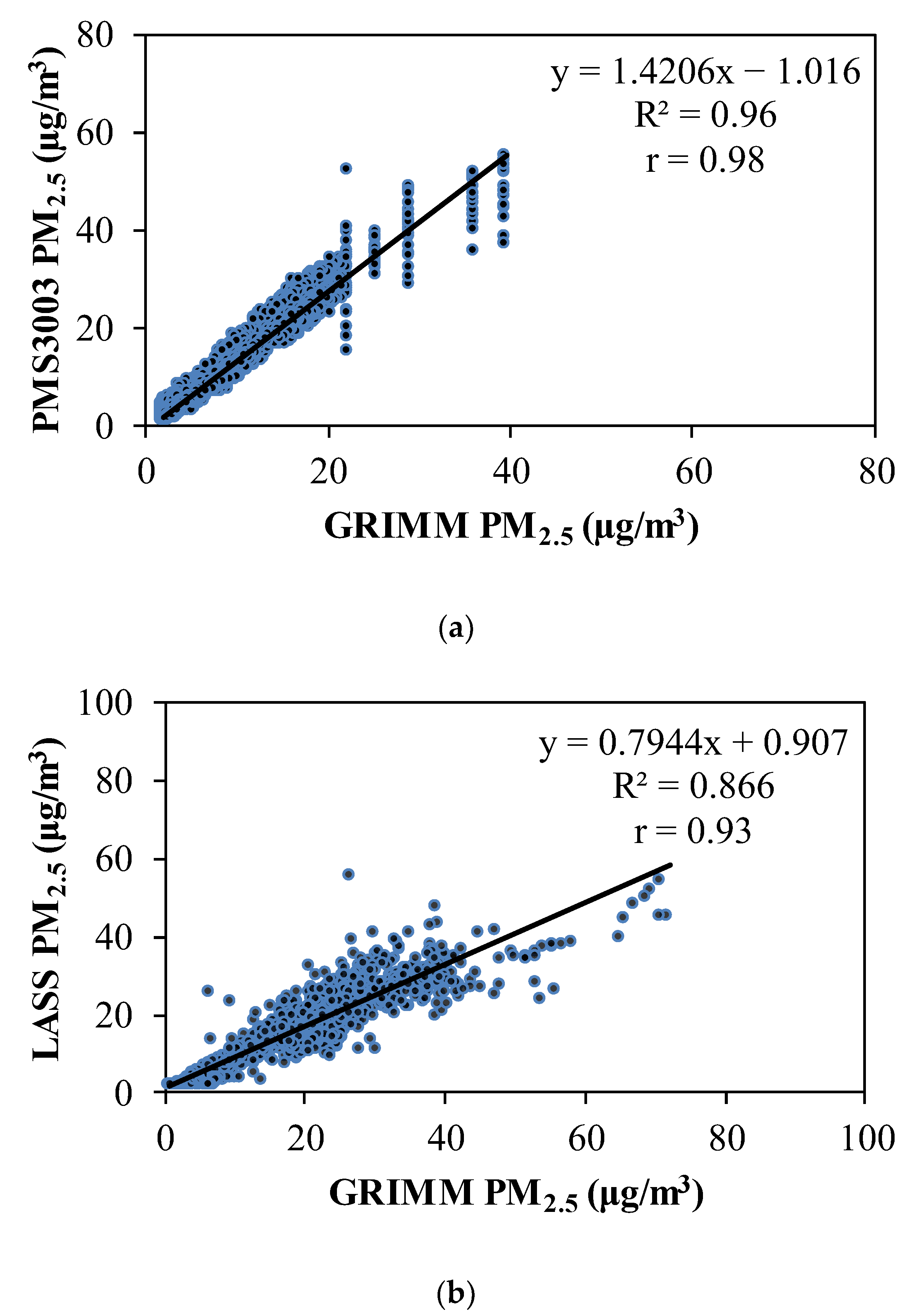
3.1. Performance Evaluation

In the laboratory tests, the r value of 5 min PM_2.5 between PMS3003 and GRIMM was 0.98 with small intercepts (Figure 2a). Although PMS3003 overestimates PM_2.5, its good precision allows conversion between PMS3003 and GRIMM measurements with the established regression. The mean absolute error (MAE) between converted PMS3003 data and GRIMM measurements was 0.85 µg/m³. Moreover, inter-sensor variability was assessed as the percentage coefficient of variation (%CV = standard deviation/mean (%)) of the 5 min averages of 16 sensors. The mean %CV of PM_2.5 among 16 sensors in the entire testing period was only 20% ± 12%. Only one regression equation was established for the correction of PM_2.5 (Figure 2a).

In fieldwork, one GRIMM and one LASS were evaluated in pairs in the six transportation modes under ambient conditions with temperatures of 23.4–42.5 °C, RH of 25.2–84.4% and PM_2.5 concentrations of 0.7–72.1 µg/m³ (see details in SM). After adjustment by regression in Figure 2a (obtained under similar RH conditions as those in the field), 5 min PM_2.5 of the converted LASS and GRIMM in field campaigns had highly correlated (r = 0.93, Figure 2b, n = 1673), with a slope of 0.7944. Additionally, the mean absolute percent difference between these two devices (absolute value of (GRIMM-LASS)/GRIMM (%)) was 21% ± 18% for 5 min PM_2.5.

It should be noted that certain discrepancies in measurements may be caused by LASS being worn near the chest and GRIMM near the waist. Moreover, different PM_2.5 levels may have been encountered when two staff carrying GRIMM and LASS were forced apart by traffic or crowds. Considering 6% ± 6% differences in previously paired PEMs [42], the absolute percentage difference of 21% ± 18% for 5 min PM_2.5 between GRIMM and LASS was deemed acceptable. The MAE between LASS and GRIMM was only 3.3 μg/m³ as shown in Table S4. Compared to the reported side-by-side comparisons between LCSs and research-grade instruments with R² reaching 0.89, MAE values reaching 5.7–14.6 μg/m³ and relative errors reaching 9–55% [16,21,30], our results revealed good performance of LASS.

In addition, it was evaluated whether temperature and RH affected the relationship of GRIMM and LASS measurements with the Equation (2). There were 40.9% of the measurements obtained under the conditions of RH above 60%. The regression coefficients of temperature and RH were mostly statistically insignificant (p-value > 0.05) (Table S5), except RH in the car mode with a coefficient of 0.04 (p-value ≤ 0.05), which was under air-conditioning. Therefore, temperature and RH were considered to have very minor effects on the relationship of GRIMM and LASS in the study. Thus, for LASS conversion, we applied the regression line in Figure 2a without temperature and humidity adjustment.

One critique might be that the present laboratory evaluation was not under prescribed temperature and humidity conditions. Taiwan has high humidity all year [43]; therefore, some instruments that have good performance under those prescribed conditions may not function well in Taiwan. This work aimed to test LASS under the actual environmental conditions to ensure the applicability of the developed device in Taiwan. The RH (the environmental factor considered to affect the PM LCS performance most) and PM_2.5 concentrations in the laboratory have covered the majority of the humidity and PM_2.5 concentrations in field campaigns. Most importantly, in-field LASS readings converted with the correction equation obtained in the laboratory had good agreement with in-field GRIMM measurements, demonstrating the applicability of the correction equation obtained in the laboratory and the reliability of LASS under the actual environmental conditions.

In terms of wearability, in contrast to GRIMM and PEM, which are (with the addition of a pump) nearly 2–2.5 kg in weight, LASS weighs under 400 g together with the mobile battery and is free of vibration and noise, making it less disturbing than GRIMM and PEM. In terms of data recovery, percentage completeness for MRT, bus, car, scooter, bike and walk were 91.9, 91.6, 82.8, 86.2, 88.8 and 91.0%, respectively. Data loss was mainly attributed to unstable wireless transmission. For measurement reliability, no ghost peaks or negative values were found.

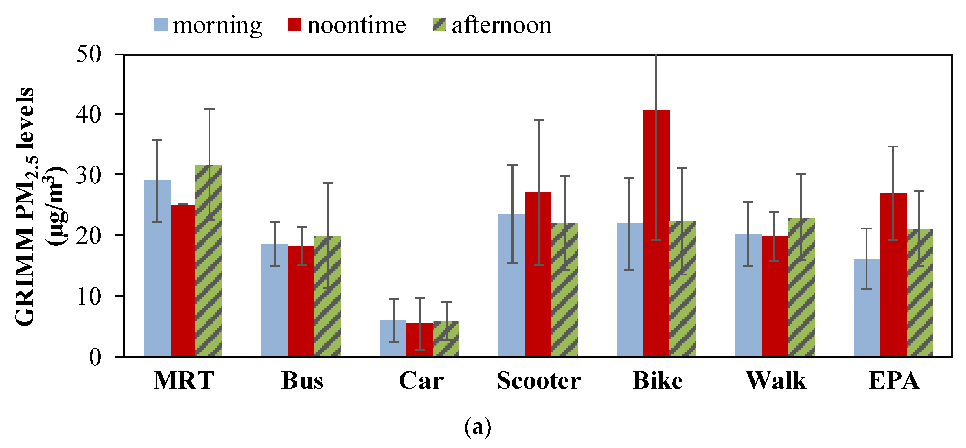
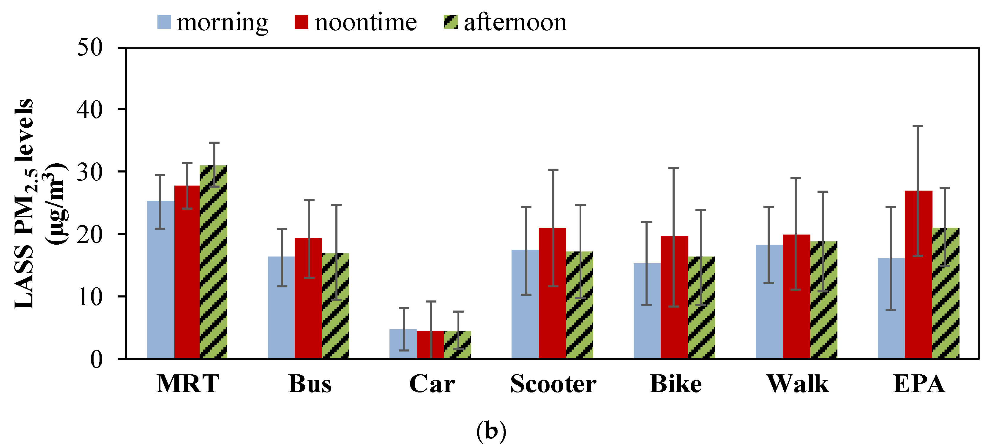
3.2. PM Exposure Levels in Six Transportation Modes

The mean 5 min PM concentrations in all monitoring trips averaged across six transportation modes were 16.9 ± 11.7 µg/m³ (n = 1774) for PM_2.5 and 21.4 ± 14.2 µg/m³ for PM₁₀ (n = 1774) with GRIMM instruments and 17.0 ± 9.5 µg/m³ (n = 3399) for PM_2.5 with LASS after conversion. Mean PM_2.5 level from LASS (17.0 µg/m³) was very close to that from GRIMM (16.9 µg/m³), with less variability due to larger sample size.

Table 1. PM exposure levels (µg/m³) in different transportation modes. (a) Hourly averages of PM with GRIMM and LASS in 2016, (b) 5 min averages of PM with GRIMM and LASS in 2016 and (c) hourly PM_2.5 with PEM in 2004 and 2005.

(a)
Mode	PM2.5 with GRIMM in 2016				PM2.5 with LASS in 2016				PM10 with GRIMM in 2016
	Mean (SD)		n		Mean (SD)		n		Mean (SD)		n
MRT	29.6	(8.0)	11		27.6	(4.7)	53		35.4	(8.9)	11
Bus	20.8	(7.5)	13		17.2	(6.2)	53		27.9	(7.3)	13
Car	5.6	(3.6)	62		4.6	(3.3)	60		6.7	(4.0)	62
Scooter	22.7	(8.9)	58		18.0	(7.9)	57		28.4	(9.5)	58
Bike	25.9	(14.6)	14		16.9	(8.3)	56		34.1	(16.2)	14
Walk	21.3	(6.3)	12		18.8	(7.6)	58		29.4	(7.6)	12
(b)
Mode	PM2.5 with GRIMM in 2016				PM2.5 with LASS in 2016				PM10 with GRIMM in 2016
	Mean (SD)		Max/Mean 1 (Range) 2	n	Mean (SD)		Max/Mean (Range)	n	Mean (sd)		Max/Mean (Range)	n
MRT	29.8	(9.2)	(1.1, 1.3)	114	27.6	(5.4)	(1.0, 1.4)	565	35.5	(10.4)	(1.1, 1.3)	114
Bus	19.9	(8.0)	(1.1, 1.7)	120	17.5	(7.1)	(1.0, 1.9)	493	27.0	(11.7)	(1.2, 3.1)	120
Car	5.9	(4.2)	(1.0, 3.4)	666	4.9	(4.0)	(1.0, 3.6)	614	7.1	(5.6)	(1.1, 5.2)	666
Scooter	22.3	(9.5)	(1.0, 2.3)	614	17.8	(8.3)	(1.0, 2.7)	574	28.2	(11.9)	(1.0, 3.2)	614
Bike	25.7	(13.7)	(1.0, 1.2)	122	17.2	(8.4)	(1.0, 2.7)	541	34.2	(16.0)	(1.0, 1.9)	122
Walk	21.3	(6.9)	(1.1, 1.4)	138	18.6	(8.0)	(1.0, 2.1)	612	29.6	(10.2)	(1.2, 2.9)	138
(c)
Mode	PM2.5 with PEM in 2004						PM2.5 with PEM in 2005
	Mean (SD)				n		Mean (SD)				n
MRT	128.7		(73.4)		15		68.1		(33.7)		15
Bus	-		-		-		-		-		-
Car	104.5		(64.0)		15		75.6		(35.1)		15
Scooter	179.8		(70.2)		14		153.3		(67.2)		15
Bike	-		-		-		-		-		-
Walk	-		-		-		-		-		-

¹ max/mean: maximum PM_2.5 /mean PM_2.5 of a one-hour trip; ² (Range) presents the minimum value of the max/mean to the maximum value of the max/mean

a presents hourly averages of PM exposures for different transportation modes from both GRIMM and converted LASS. The lowest PM_2.5 means were observed for car drivers, while the highest occurred in MRT, with either LASS or GRIMM; the same pattern holds for PM₁₀ with GRIMM. Additionally, larger variability was observed for PM_2.5 and PM₁₀ exposures of scooter riders and bikers with both GRIMM and LASS compared with other modes, presumably due to closer contact with vehicle emissions. The 5 min PM_2.5 levels which were obtained from LASS for scooter riders and bikers were 4.6 and 5.3 µg/m³ lower than those from GRIMM (paired t-tests, p-value ≤ 0.05), respectively, while those in the other four modes were not statistically significantly different (Table 1b). It was speculated that GRIMM worn at the waist may be closer to vehicle emissions near the ground. In the other four modes with more homogeneous PM_2.5 concentrations, converted LASS readings were very close to those of GRIMM.

To avoid the influence of speed fluctuation on measurements, the staff carrying GRIMM and LASS were instructed to drive at a stable speed and not too fast. The speed limit was 50 km/hr on the planned route. The speeds were maintained below 40 km/hr for scooter riders and below 10 km/hr for bikers, except when being stopped by traffic lights. In addition, PMS3003 with a volume-scattering detection approach obtained PM measurements independent of the flow rate [44]. Thus, our results were not significantly affected by the speed fluctuation.

The ratios of the maximum 5 min PM_2.5 during a one-hour trip over the mean PM_2.5 levels were calculated. The maximum of the max/mean ratios were 1.4, 1.9, 3.6, 2.7, 2.7 and 2.1 for MRT, bus, car, scooter, bike and walking, respectively (Table 1b). The difference between peak and mean exposure levels could be as large as 3.6-fold. Direct exposure to traffic exhaust caused 2.1–2.7-fold differences for commuters in scooter, bike and walking modes. Integrated personal samplers such as PEM would miss the important characteristics of peak exposures. LASS can assess peak exposures and pinpoint the activities or environmental conditions the peaks occur.

Comparing the present measurements with 2004–2005 campaigns shows much lower exposure levels in 2016 (Table 1c). In addition, although exposures of car drivers remained the lowest, the exposures of scooter riders were higher than those of MRT riders in 2004–2005 with opposite patterns in 2016. Ambient PM_2.5 levels have decreased over these 12 years (Table S3), with levels in 2004 (26.8 µg/m³) and 2005 (49.2 µg/m³) being 144% and 266% higher than those in 2016 (18.5 µg/m³), respectively. The dramatic reduction in PM_2.5 exposures of scooter riders was likely due to ambient PM_2.5 decrease, while the MRT users may have been exposed to other indoor sources [36], resulting in higher exposures than those of scooter riders in 2016.

Figure 3a,b show exposures in the six transportation modes with GRIMM and LASS, respectively, along with EPA data. Higher exposures were observed in certain transportation modes in rush hours compared to EPA levels. This was attributed to subjects being in closer proximity to emission sources during commuting. Moreover, the relative comparison of observations between different transportation modes at different periods from LASS readings were similar to those from GRIMM.

Regression analysis performed on LASS observations shows that the average hourly exposure increments with MRT, bus, car, scooter, bike and walking were 15.6, 6.7, −19.2, 8.1, 6.1 and 7.1 µg/m³, respectively, very close to those obtained from GRIMM (

Table 2. T Hourly exposure increments (µg/m³) from different transportation modes with (a) GRIMM (n = 155, adj R² = 0.65) and (b) LASS (n = 309, adj R² = 0.62).

(a)
Mode	Parameter Estimate	Standard Error	p-Value
Intercept (car)	−26.7	15.2	0.081
MRT	15.9	3.9	0.000
Bus	4.6	3.8	0.226
Scooter	9.9	4.8	0.040
Bike	9.3	5.1	0.068
Walk	4.9	5	0.329
Air temperature	−0.1	0.4	0.843
Relative Humidity	0.4	0.1	0.002
(b)
Mode	Parameter Estimate	Standard Error	p-Value
Intercept (car)	−19.2	11.4	0.095
MRT	15.6	2.4	0.000
Bus	6.7	2.6	0.010
Scooter	8.1	3.6	0.025
Bike	6.1	3.6	0.092
Walk	7.1	3.6	0.048
Air temperature	−0.3	0.3	0.261
Relative Humidity	0.3	0.1	0.000

a,b). With GRIMM, statistically significant coefficients were only obtained for the MRT and scooter modes at p-value ≤ 0.05 and for the bike mode at p-value ≤ 0.10. The high cost limits the use of multiple sets of GRIMM to conduct parallel monitoring and obtain sample sizes large enough for statistically significant estimations of the coefficients. However, multiple LASS sets can be applied in parallel to obtain the coefficients with statistical significance for modes of MRT, bus, scooter and walking at p-value ≤ 0.05 and for the modes of car and bike at p-value ≤ 0.10. The exposure increment for the scooter mode is higher from GRIMM compared to that from LASS, possibly because GRIMM was carried in the front seat, exposing it to higher PM_2.5 compared to LASS, which was in the back seat.

PM_2.5 exposures in the six transportation modes were compared with those from previous studies. Kumar et al. [36] comprehensively reviewed and summarized exposures in different transportation modes in Asia in comparison with the USA and Europe up to 2015 (

Table 3. PM_2.5 concentrations in multiple transportation modes summarized from the literature.

Location	Transportation Mode						Instrument	Year of Field Work	Reference
	Subway	AC Bus	AC Car	Scooter	Bike	Walk
Asia, review	-	76 (62)	74 (61)	86.3 (55.7)	49 (27)	42 (31)	varied instrument 1	before 2014	Kumar et al. [36]
Beijing, China	61.8 (21.6)	38.9 (26.3)	-	-	-	49.9 (51.7)	TSI DustTrak	2011	Yan et al. [34]
Delhi, India	-	315 (105)	-	-	347 (94)	231 (72)	TSI DustTrak	2014	Goel et al. [35] January
Delhi, India	87 (141)	140 (56)	56 (44)	-	-	234 (184)	TSI DustTrak	2014	Goel et al. [35] April
Hong Kong	19 (1.1)	19 (2.1)	-	-	-	38 (3.2)	TSI DustTrak II	2014	Che et al. [45] lunchtime
Hong Kong	23 (1.5)	-	-	-	-	43 (3.6)	TSI DustTrak II	2014	Che et al. [45] evening
Hong Kong	31 (13)	39 (21)	-	-	-	-	TSI DustTrak	2015	Li et al. [46]
Xian, China	43.2 (24.2)	54.4 (7.15)	10.1 (6.63)	-	-	71.6 (5.11)	GRIMM 1.109	2016	Qiu et al. [47] morning
Xian, China	43.4 (9.72)	-	8.95 (1.08)	-	-	65.8 (11.0)	GRIMM 1.109	2016	Qiu et al. [47] afternoon
US, review	-	59 (59)	46 (36)	-	11 (5)	35 (13)	varied instrument 1	before 2014	Kumar et al. [36]
Sacramento, CA, US	-	7.47 (2)	7.1 (3.3)	-	9.56 (4)	-	TSI DustTrak	2014-2015	Ham et al. [48]
Europe, review	-	47 (37)	32 (30)	-	43 (27)	26 (18)	varied instrument 1	before 2014	Kumar et al. [36]
London, UK 2	34.5 (2.9)	13.9 (1.7)	7.3 (2)	-	-	-	GRIMM EDM 107	2016	Rivas et al. [49]

¹ These were obtained from different studies with various instruments such as TSI DustTrak and GRIMM; ² Data with geometric mean and geometric standard deviation.

). Research articles focusing on PM_2.5 exposures in multiple transportation modes in cities of Asia, USA and Europe using wearable or portable sensing devices with conditions similar to ours are also listed [34,35,45,46,47,48,49].

For the subway, 5 min PM_2.5 exposures from GRIMM (29.8 ± 9.2 µg/m³) and LASS (27.6 ± 5.4 µg/m³) in Taipei were similar to those in Hong Kong 2015 and London, UK; higher than those in Hong Kong in 2014; and lower than those in Beijing and Xian, China and Delhi, India. The highest PM_2.5 exposures occurred in Delhi, India, with 87 ± 141 µg/m³, about 3 times those in Taipei. For the AC bus mode, 5 min PM_2.5 exposures from GRIMM (19.9 ± 8.0 µg/m³) and LASS (17.5 ± 7.1 µg/m³) in Taipei were similar to those in Hong Kong 2014; higher than those in Sacramento, CA, USA and London, UK; and lower than those in Hong Kong 2015, Beijing and Xian, China, Delhi, India and Asia, Europe and USA in general. Again, Delhi, India had the highest PM_2.5 exposures, with one order of magnitude higher than our results in Taipei. Therefore, commuters in subways and buses, the most commonly used public transportation systems in Taipei, were generally exposed to lower PM_2.5 levels compared to those in other countries with few exceptions. Characteristics of subway systems such as wear processes at rail–wheel–brake interfaces, construction dates, existence of platform edge doors, ventilation systems and passenger volume may explain the differences of their PM_2.5 exposures [34,47,49,50,51]. In addition, diversities in fuel specifications and emission standards among countries may explain the large variations of PM_2.5 exposures in AC buses across Asia [36].

For AC cars, 5 min PM_2.5 exposures from GRIMM (5.9 ± 4.2 µg/m³) and LASS (4.9 ± 4.0 µg/m³) in Taipei were lower than most of the published values and less than 1/10 of the highest reported PM_2.5 exposure levels, namely the summarized means in Asia (without specified ventilation status mentioned) [36]. For scooters, 5 min PM_2.5 exposures were 22.3 ± 9.5 µg/m³ (GRIMM) and 17.8 ± 8.3 µg/m³ (LASS) in Taipei, less than 1/4 of the summarized values in Asia of 86.3 ± 55.7 µg/m³. Generally speaking, car drivers and scooter riders in Taipei had much lower exposures than those reported in Asia. The practices of keeping windows closed with re-circulated AC in cars and the relatively clean ambient air may explain these low PM_2.5 exposures in Taipei.

The bikers’ 5 min PM_2.5 exposures of 25.7 ± 13.7 µg/m³ (GRIMM) and 17.2 ± 8.4 µg/m³ (LASS) in Taipei were higher than those reported in the USA but lower than those in Asia and Europe. The pedestrians’ 5 min PM_2.5 exposures of 21.3 ± 6.9 µg/m³ (GRIMM) and 18.6 ± 8.0 µg/m³ (LASS) in Taipei were lower than those reported. The highest PM_2.5 exposures of both bikers and pedestrians were in Delhi, India, at one order of magnitude higher than ours. Since bikers and pedestrians were directly exposed to the street air with traffic exhaust, the relative PM_2.5 exposures among different cities could represent their relative urban PM_2.5 levels in the streets.

In terms of comparison among different transportation modes, we focus on exposures of single cities [34,35,45,46,47,48,49] rather than the summarized means in the review [36]. Commuters in AC cars had the lowest PM_2.5 exposures among the transportation modes studied, consistent with our findings. The commuters’ exposures in the subway mode were the highest compared to the modes of walking and AC buses in Beijing, China [34], with the same order as ours. The subway riders’ exposures in London, UK were higher than those on AC buses and in AC cars [49], also with the same order as ours.

Previously, PM_2.5 measurements in multiple transportations modes were performed using large and pricy instruments (much more than 500 USD) such as TSI or GRIMM (Table 3). With the development of LCS devices, personal PM_2.5 exposures could be more easily assessed. Portable LCSs were applied to assess personal PM_2.5 exposures in indoor, outdoor and commuting microenvironments [52,53]. For the measurement of personal PM_2.5 increments by traffic, portable LCS devices serve as a more flexible option compared to stationary ones [40]. Although portable LCS devices have been increasingly applied for personal PM_2.5 exposure assessments, mainly daily exposures were measured and studies on individual transportation modes seem few. For example, PM_2.5 exposures of 73 subjects for 4 days in Hong Kong in 2015–2016 was assessed using Alphasense OPC-N2, a type of LCS [54]; R² of side-by-side comparison between the sensors and pDR-1500 ranged from 0.95 to 0.99. In another study, 31 subjects carried a portable aerosol nephelometer for their exposure measurements of PM₁, PM_2.5 and PM₁₀ in Beijing in 2018 and this sensor was compared with TSI DustTrank showing R² ranging from 0.49 to 0.66, not as good as the performance of PMS3003 [55]. Our present work is markedly one of the earliest studies to apply wearable LCS devices for the assessment of PM_2.5 exposures in different transportation modes.

Furthermore, this work contributes to fill the current research gaps of pedestrians’ and cyclists’ exposures in Asian cities [36]. In Taipei City, pedestrians are mostly walking on narrowed sidewalks in close proximity to traffic. In addition, there are bike lanes on the sidewalks of some streets. Moreover, pedestrians, cyclists and scooter riders all need to gather near the traffic-light zones when crossing the streets and are thus exposed to concentrated PM emissions from the crowded vehicles, resulting in similar mean or even peak exposures among them. Nevertheless, if exposure duration is taken into account, it takes longer for pedestrians to reach the same destination. Therefore, for cumulative exposures (µg/m³-hr) on the same route, pedestrians are exposed to higher total exposure.

Attempts have been made to quantify the contribution of different transportation modes to human exposures with different methods, such as time series analysis and ratio calculation (e.g., [35,49]). This work used regression analysis to quantify exposure increments. With LASS applied to collect data with a larger sample size, the standard errors of the contribution estimates of transportation modes are reduced. This also widens the application of LASS in PM_2.5 exposure assessment in locations with potentially high exposure sources, such as restaurants, temples and so forth.

Although personal exposures in transportation microenvironments are influenced by several factors [36], the exposure patterns among different transportation modes mostly still hold for the same city of the same season in the same year. Moreover, the quantified exposure levels can be used by the authorities to support the necessary control strategies such as implementing countermeasures to reduce exposure increments of MRT users. Furthermore, quantitative evidence would convince the public more easily of the need for behavioral changes to reduce exposure increments and associated health risks. In this case, the potential behavioral changes may be avoiding crowded environments in front of traffic lights and wearing masks in the MRT.

3.3. Advantages and Disadvantages of LASS

No ghost peak was observed with the easy-to-carry LASS under movements in these transportation modes. The r values of PM_2.5 between PMS3003 and GRIMM were 0.98 and 0.93 in the laboratory and field, respectively. With good precision, accuracy, stability and wearability, LASS provided a promising alternative for scientists to obtain real-time PM_2.5 exposure data if expensive instruments, such as GRIMM, could not be afforded.

Exposure scientists expect subjects to maintain their daily routines. However, due to the heavy weight, bulkiness and striking look of traditional instruments like GRIMM and PEM, subjects carrying these instruments may shy away from crowded environments and avoid activities involving more movements, thus missing certain high-exposure activities. The wearability of LASS near the breathing zone allows subjects to maintain their daily routines so that scientists can identify/evaluate PM_2.5 increments of high-exposure activities such as visiting night markets which might be skipped if wearing traditional instruments. Thus, the first advantage of LASS is enabling scientists to assess the close-to reality exposures of subjects. Moreover, the light-weight and free-of-vibration-and-noise LASS provides enhanced incentives for the participation of the targeted population, thus increasing sample size (second advantage). With cost reduction, scientists can also afford to conduct more sets of parallel monitoring to collect more data with higher statistical power and lower errors of regression estimates for differentiating the exposures in different categories of microenvironments, in this case, transportation modes.

Furthermore, new features of LASS provide greater potential to reduce data loss and to assess exposure factors. For example, wireless transmission in real time allows scientists to check on data and to identify potential problems immediately to minimize data loss. Additionally, more information such as temperature, humidity and GPS can be collected by a single device to assess potential factors. Besides, the mean time to failure of PMS3003 is over 3 years as reported by the manufacturer [56] and based on own experiences. Since sensor evaluation is time- and resource-consuming, applying a stable LCS is more important than using new ones with unknown drawbacks.

There are other drawbacks associated with the current version of LASS. During the trials, up to one-third of the data in one trip were lost due to unstable wireless transmission. This issue was solved by repeated checking on transmission and data in cloud storage throughout the monitoring periods. Development of an improved version with a memory card was also suggested to reduce data loss. Secondly, some of the laboratory-made LASS devices had unstable electric connections. As a result, about 10% of the devices malfunctioned in the trial. This could be improved by a customer-made production from a machine shop to ensure a smooth electric connection. Moreover, LASS still needs to be compared against a research-grade instrument for data correction. The side-by-side comparison in the laboratory and field takes both time and manpower, which also need to be taken into account by scientists intending to use these devices.

4. Conclusions

This work demonstrates a successful PM_2.5 exposure assessment for commuters with LASS. The commuters’ PM_2.5 exposure levels assessed with LASS were 27.6 ± 4.7, 17.2 ± 6.2, 4.6 ± 3.3, 18.0 ± 7.9, 16.9 ± 8.3 and 18.8 ± 7.6 µg/m³ for MRT, bus, car, scooter, bike and walking, respectively. These exposure levels and the exposure increments assessed with LASS and GRIMM were very close to each other. These results showed that LASS can be used as an alternative for exposure studies.

The advantages of applying low-cost, light-weight, easy-to-carry and free-of-vibration-and-noise LASS to exposure assessment include (1) assessing actual and typical exposure levels in high-exposure situations without interfering with daily routines of subjects; (2) easier recruiting of subjects and conducting more sets of parallel monitoring to increase statistical power for differentiating exposure factors; and (3) collecting other parameters at the same time. Especially for developing countries with high-PM_2.5 levels, LASS is a good scientific tool to measure PM_2.5 exposures with a much lower cost than traditional instruments. This work is one of the earliest demonstrating the applicability of a wearable LCS device, LASS, in assessing human exposure in different transportation modes in high spatiotemporal resolutions. The methodology and findings would shed light on the potential applications of the wearable LCS in PM exposure assessment.

References

1. Brauer, M.; Freedman, G.; Frostad, J.; Van Donkelaar, A.; Martin, R.V.; Dentener, F.; Van Dingenen, R.; Estep, K.; Amini, H.; Apte, J.S.; et al. Ambient Air Pollution Exposure Estimation for the Global Burden of Disease 2013. Environ. Sci. Technol. 2016, 50, 79–88. [Google Scholar] [CrossRef]
2. Van Donkelaar, A.; Martin, R.V.; Brauer, M.; Boys, B.L. Use of Satellite Observations for Long-Term Exposure Assessment of Global Concentrations of Fine Particulate Matter. Environ. Health Perspect. 2015, 123, 135–143. [Google Scholar] [CrossRef] [Green Version]
3. World Health Organization. Ambient (Outdoor) Air Quality and Health. Available online: http://www.who.int/mediacentre/factsheets/fs313/en/ (accessed on 20 June 2020).
4. Pope, C.A., III; Dockery, D.W. Health effects of fine particulate air pollution: Lines that connect. J. Air Waste Manag. Assoc. 2006, 56, 709–742. [Google Scholar] [CrossRef] [PubMed]
5. Pope, C.A., III; Dockery, D.W.; Spengler, J.D.; Raizenne, M.E. Respiratory health and PM10 pollution: A daily time-series analysis. Am. Rev. Respir. Dis. 1991, 144, 668–674. [Google Scholar] [CrossRef]
6. United States Environmental Protection Agency (USEPA). Air Quality Criteria for Particulate Matter. Available online: https://cfpub.epa.gov/ncea/risk/recordisplay.cfm?deid=87903 (accessed on 25 June 2020).
7. Forouzanfar, M.H.; Afshin, A.; Alexander, L.T.; Anderson, H.R.; Bhutta, Z.A.; Biryukov, S.; Brauer, M.; Burnett, R.; Cercy, K.; Charlson, F.J.; et al. Global, regional and national comparative risk assessment of 79 behavioural, environmental and occupational and metabolic risks or clusters of risks, 1990–2015: A systematic analysis for the Global Burden of Disease Study. Lancet 2016, 388, 1659–1724. [Google Scholar] [CrossRef] [Green Version]
8. Lelieveld, J.; Evans, J.S.; Fnais, M.; Giannadaki, D.; Pozzer, A. The contribution of outdoor air pollution sources to premature mortality on a global scale. Nature 2015, 525, 367–371. [Google Scholar] [CrossRef] [PubMed]
9. International Agency for Research on Cancer IARC. IARC Scientific Publication No.161: Air Pollution and Cancer. Available online: http://publications.iarc.fr/Book-And-Report-Series/Iarc-Scientific-Publications/Air-Pollution-And-Cancer-2013 (accessed on 10 July 2020).
10. Mohammed, M.O.A.; Song, W.W.; Ma, W.L.; Li, W.L.; Ambuchi, J.J.; Thabit, M.; Li, Y.-F. Trends in indoor-outdoor PM2.5 research: A systematic review of studies conducted during the last decade (2003–2013). Atmos. Pollut. Res. 2015, 6, 893–903. [Google Scholar] [CrossRef]
11. Lung, S.-C.C.; Mao, I.-F.; Liu, L.-J.S. Residents’ particle exposures in six different communities in Taiwan. Sci. Total Environ. 2007, 377, 81–92. [Google Scholar] [CrossRef]
12. Lung, S.-C.C.; Hsiao, P.-K.; Wen, T.-Y.; Liu, C.-H.; Fu, C.B.; Cheng, Y.-T. Variability of intra-urban exposure to particulate matter and CO from Asian-type community pollution sources. Atmos. Environ. 2014, 83, 6–13. [Google Scholar] [CrossRef] [Green Version]
13. Jerrett, M.; Burnet, R.T.; Ma, R.; Pope, C.A., III; Krewski, D.; Newbold, B.; Thurston, G.; Shi, Y.; Finkelstein, N.; Calle, E.E.; et al. Spatial analysis of air pollution and mortality in Los Angeles. Epidemiology 2006, 17, S69. [Google Scholar] [CrossRef]
14. Pope, C.A., III; Burnett, R.T.; Thun, M.J.; Calle, E.E.; Krewski, D.; Ito, K.; Thurston, G.D. Lung cancer, cardiopulmonary mortality and long-term exposure to fine particulate air pollution. JAMA 2002, 287, 1132–1141. [Google Scholar] [CrossRef] [Green Version]
15. Snyder, E.G.; Watkins, T.H.; Solomon, P.A.; Thoma, E.D.; Williams, R.W.; Hagler, G.S.W.; Shelow, D.; Hindin, D.A.; Kilaru, V.J.; Preuss, P.W. The Changing Paradigm of Air Pollution Monitoring. Environ. Sci. Technol. 2013, 47, 11369–11377. [Google Scholar] [CrossRef]
16. Gao, M.; Cao, J.; Seto, E. A distributed network of low-cost continuous reading sensors to measure spatiotemporal variations of PM2.5 in Xi’an, China. Environ. Pollut. 2015, 199, 56–65. [Google Scholar] [CrossRef] [PubMed] [Green Version]
17. Holstius, D.M.; Pillarisetti, A.; Smith, K.R.; Seto, E. Field calibrations of a low-cost aerosol sensor at a regulatory monitoring site in California. Atmos. Meas. Tech. 2014, 7, 1121–1131. [Google Scholar] [CrossRef] [Green Version]
18. Clements, A.L.; Griswold, W.G.; Rs, A.; Johnston, J.E.; Herting, M.M.; Thorson, J.; Collier-Oxandale, A.; Hannigan, M. Low-Cost Air Quality Monitoring Tools: From Research to Practice (A Workshop Summary). Sensors 2017, 17, 2478. [Google Scholar] [CrossRef] [Green Version]
19. Austin, E.; Novosselov, I.; Seto, E.; Yost, M.G. Laboratory evaluation of the Shinyei PPD42NS low-cost particulate matter sensor. PLoS ONE 2015, 10, e0141928. [Google Scholar]
20. Cao, T.; Thompson, J.E. Portable, Ambient PM2.5 Sensor for Human and/or Animal Exposure Studies. Anal. Lett. 2017, 50, 712–723. [Google Scholar] [CrossRef]
21. Wang, Y.; Li, J.; Jing, H.; Zhang, Q.; Jiang, J.; Biswas, P. Laboratory Evaluation and Calibration of Three Low-Cost Particle Sensors for Particulate Matter Measurement. Aerosol Sci. Technol. 2015, 49, 1063–1077. [Google Scholar] [CrossRef]
22. Badura, M.; Batog, P.; Drzeniecka-Osiadacz, A.; Modzel, P. Evaluation of Low-Cost Sensors for Ambient PM2.5 Monitoring. J. Sens. 2018, 2018, 1–16. [Google Scholar] [CrossRef] [Green Version]
23. Air Quality Sensor Performance Evaluation Center. PM Sensor Evaluations. Available online: http://www.aqmd.gov/aq-spec/evaluations/summary-pm (accessed on 20 July 2020).
24. Kuula, J.; Mäkelä, T.; Aurela, M.; Teinilä, K.; Varjonen, S.; González, Ó.; Timonen, H. Laboratory evaluation of particle-size selectivity of optical low-cost particulate matter sensors. Atmos. Meas. Tech. 2020, 13, 2413–2423. [Google Scholar] [CrossRef]
25. United States Environmental Protection Agency USEPA. Quality Assurance Handbook for Air Pollution Measurement Systems: “Volume Ⅱ: Ambient Air Quality Monitoring Program”. Available online: https://www3.epa.gov/ttn/amtic/qalist.html (accessed on 9 September 2019).
26. United States Environmental Protection Agency USEPA. Air Sensor Guidebook. Available online: https://cfpub.epa.gov/si/si_public_record_report.cfm?Lab=NERL&dirEntryId=277996 (accessed on 9 September 2019).
27. Jayaratne, R.; Liu, X.; Ahn, K.-H.; Asumadu-Sakyi, A.; Fisher, G.; Gao, J.; Mabon, A.; Mazaheri, M.; Mullins, B.; Nyaku, M.; et al. Low-cost PM2.5 Sensors: An Assessment of Their Suitability for Various Applications. Aerosol Air Qual. Res. 2020, 20, 520–532. [Google Scholar] [CrossRef]
28. Kelly, K.; Whitaker, J.; Petty, A.; Widmer, C.; Dybwad, A.; Sleeth, D.; Martin, R.; Butterfield, A. Ambient and laboratory evaluation of a low-cost particulate matter sensor. Environ. Pollut. 2017, 221, 491–500. [Google Scholar] [CrossRef] [PubMed]
29. Chen, L.-J.; Ho, Y.-H.; Lee, H.-C.; Wu, H.-C.; Liu, H.-M.; Hsieh, H.-H.; Huang, Y.-T.; Lung, S.-C.C. An Open Framework for Participatory PM2.5 Monitoring in Smart Cities. IEEE Access 2017, 5, 14441–14454. [Google Scholar] [CrossRef]
30. Borghi, F.; Spinazzè, A.; Campagnolo, D.; Rovelli, S.; Cattaneo, A.; Cavallo, D.M. Precision and Accuracy of a Direct-Reading Miniaturized Monitor in PM2.5 Exposure Assessment. Sensors 2018, 18, 3089. [Google Scholar] [CrossRef] [Green Version]
31. Han, I.; Symanski, E.; Stock, T.H. Feasibility of using low-cost portable particle monitors for measurement of fine and coarse particulate matter in urban ambient air. J. Air Waste Manag. Assoc. 2016, 67, 330–340. [Google Scholar] [CrossRef] [Green Version]
32. Liu, H.-Y.; Schneider, P.; Haugen, R.; Vogt, M. Performance Assessment of a Low-Cost PM2.5 Sensor for a near Four-Month Period in Oslo, Norway. Atmosphere 2019, 10, 41. [Google Scholar] [CrossRef] [Green Version]
33. Wang, W.-C.V.; Lung, S.-C.C.; Liu, C.H.; Shui, C.-K. Laboratory Evaluations of Correction Equations with Multiple Choices for Seed Low-Cost Particle Sensing Devices in Sensor Networks. Sensors 2020, 20, 3661. [Google Scholar] [CrossRef] [PubMed]
34. Yan, C.; Zheng, M.; Yang, Q.; Zhang, Q.; Qiu, X.; Zhang, Y.; Fu, H.; Li, X.; Zhu, T.; Zhu, Y. Commuter exposure to particulate matter and particle-bound PAHs in three transportation modes in Beijing, China. Environ. Pollut. 2015, 204, 199–206. [Google Scholar] [CrossRef]
35. Goel, R.; Gani, S.; Guttikunda, S.K.; Wilson, D.; Tiwari, G. On-road PM2.5 pollution exposure in multiple transport microenvironments in Delhi. Atmos. Environ. 2015, 123, 129–138. [Google Scholar] [CrossRef]
36. Kumar, P.; Patton, A.P.; Durant, J.L.; Frey, H.C. A review of factors impacting exposure to PM2.5, ultrafine particles and black carbon in Asian transport microenvironments. Atmos. Environ. 2018, 187, 301–316. [Google Scholar] [CrossRef]
37. Location-Aware Sensing System (LASS). Available online: https://lass-net.org/ (accessed on 15 August 2020).
38. Liang, C.-S.; Yu, T.-Y.; Chang, Y.-Y.; Syu, J.-Y.; Lin, W.-Y. Source Apportionment of PM2.5 Particle Composition and Submicrometer Size Distribution during an Asian Dust Storm and Non-Dust Storm in Taipei. Aerosol Air Qual. Res. 2013, 13, 545–554. [Google Scholar] [CrossRef] [Green Version]
39. Sayahi, T.; Butterfield, A.; Kelly, K. Long-term field evaluation of the Plantower PMS low-cost particulate matter sensors. Environ. Pollut. 2019, 245, 932–940. [Google Scholar] [CrossRef]
40. Lung, S.C.C.; Wang, W.C.V.; Wen, T.Y.J.; Liu, C.H.; Hu, S.C. A versatile low-cost sensing device for assessing PM2.5 spatio-temporal variation and quantifying source contribution. Sci. Total Environ. 2020, 716, 137145. [Google Scholar] [CrossRef]
41. Zwack, L.M.; Paciorek, C.J.; Spengler, J.D.; Levy, J.I. Characterizing local traffic contributions to particulate air pollution in street canyons using mobile monitoring techniques. Atmos. Environ. 2011, 45, 2507–2514. [Google Scholar] [CrossRef]
42. Lung, S.-C.C.; Kao, M.-C. Worshippers’ exposure to particulate matter in two temples in Taiwan. J. Air Waste Manag. Assoc. 2003, 53, 130–135. [Google Scholar] [CrossRef] [Green Version]
43. Taiwan Central Weather Bureau. Monthly Mean Temperature. Available online: https://www.cwb.gov.tw/V8/E/C/Statistics/monthlymean.html (accessed on 30 July 2020).
44. Zheng, T.; Bergin, M.H.; Johnson, K.K.; Tripathi, S.N.; Shirodkar, S.; Landis, M.S.; Sutaria, R.; Carlson, D.E. Field evaluation of low-cost particulate matter sensors in high- and low-concentration environments. Atmos. Meas. Tech. 2018, 11, 4823–4846. [Google Scholar] [CrossRef] [Green Version]
45. Che, W.; Frey, H.C.; Lau, A.K.H. Sequential Measurement of Intermodal Variability in Public Transportation PM2.5 and CO Exposure Concentrations. Environ. Sci. Technol. 2016, 50, 8760–8769. [Google Scholar] [CrossRef]
46. Li, Z.Y.; Che, W.W.; Frey, H.C.; Lau, A.K.H.; Lin, C.Q. Characterization of PM2.5 exposure concentration in transport micro-environments using portable monitors. Environ. Pollut. 2017, 228, 433–442. [Google Scholar] [CrossRef]
47. Qiu, Z.; Song, J.; Xu, X.; Luo, Y.; Zhao, R.; Zhou, W.; Xiang, B.; Hao, Y. Commuter exposure to particulate matter for different transportation modes in Xi’an, China. Atmos. Pollut. Res. 2017, 8, 940–948. [Google Scholar] [CrossRef]
48. Ham, W.; Vijayan, A.; Schulte, N.; Herner, J.D. Commuter exposure to PM2.5, BC and UFP in six common transport micro-environments in Sacramento, California. Atmos. Environ. 2017, 167, 335–345. [Google Scholar] [CrossRef]
49. Rivas, I.; Kumar, P.; Hagen-Zanker, A. Exposure to air pollutants during commuting in London: Are there inequalities among different socio-economic groups? Environ. Int. 2017, 101, 143–157. [Google Scholar] [CrossRef] [Green Version]
50. Grass, D.S.; Ross, J.M.; Family, F.; Barbour, J.; Simpson, H.J.; Coulibaly, D.; Hernandez, J.; Chen, Y.; Slavkovich, V.; Li, Y.; et al. Airborne particulate metals in the New York City subway: A pilot study to assess the potential for health impacts. Environ. Res. 2010, 110, 1–11. [Google Scholar] [CrossRef] [Green Version]
51. Kam, W.; Ning, Z.; Shafer, M.M.; Schauer, J.J.; Sioutas, C. Chemical Characterization and Redox Potential of Coarse and Fine Particulate Matter (PM) in Underground and Ground-Level Rail Systems of the Los Angeles Metro. Environ. Sci. Technol. 2011, 45, 6769–6776. [Google Scholar] [CrossRef] [PubMed]
52. Lung, S.C.; Tsou, M.M.; Hu, S.; Hsieh, Y.; Wang, W.V.; Shui, C.; Tan, C. Concurrent assessment of personal, indoor and outdoor PM 2.5 and PM 1 levels and source contributions using novel low-cost sensing devices. Indoor Air 2020. [Google Scholar] [CrossRef] [PubMed]
53. Chatzidiakou, L.; Krause, A.; Popoola, O.A.M.; Di Antonio, A.; Kellaway, M.; Han, Y.; Squires, F.A.; Wang, T.; Zhang, H.; Wang, Q.; et al. Characterising low-cost sensors in highly portable platforms to quantify personal exposure in diverse environments. Atmos. Meas. Tech. 2019, 12, 4643–4657. [Google Scholar] [CrossRef] [PubMed] [Green Version]
54. Yang, F.; Lau, C.F.; Tong, V.W.T.; Zhang, K.K.; Westerdahl, D.; Ng, S.; Ning, Z. Assessment of personal integrated exposure to fine particulate matter of urban residents in Hong Kong. J. Air Waste Manag. Assoc. 2018, 69, 47–57. [Google Scholar] [CrossRef] [PubMed]
55. Liang, L.; Gong, P.; Cong, N.; Li, Z.; Zhao, Y.; Chen, Y. Assessment of personal exposure to particulate air pollution: The first result of City Health Outlook (CHO) project. BMC Public Health 2019, 19, 1–12. [Google Scholar] [CrossRef] [PubMed] [Green Version]
56. Sayahi, T.; Kaufman, D.; Becnel, T.; Kaur, K.; Butterfield, A.; Collingwood, S.; Zhang, Y.; Gaillardon, P.-E.; Kelly, K. Development of a calibration chamber to evaluate the performance of low-cost particulate matter sensors. Environ. Pollut. 2019, 255, 113131. [Google Scholar] [CrossRef] [PubMed]
Figure 1. Low-cost particulate matter (PM) sensing device, Location-Aware Sensing System (LASS), used in this work; various components and the inlet/outlet of LASS are marked; sensor components and the real-time clock modules are connected to the mainboard with wires not shown in the figure to avoid blocking views of the board. PLA: polylactic acid, a material commonly used for 3D printing.
Atmosphere 12 00270 g001
Figure 2. Comparison of GRIMM with (a) PM2.5 of PMS3003 in laboratory (n = 12,208) and (b) PM2.5 of Location-Aware Sensing System (LASS) observations in field converted by the correction equation shown in (a) (n = 1673); the data presented were 5 min averages.
Atmosphere 12 00270 g002
Figure 3. PM2.5 levels in six transportation modes obtained from (a) GRIMM and (b) LASS (converted) along with those of Taiwan Environmental Protection Agency during the monitoring periods; error bars represent standard deviations of these measurements.
Atmosphere 12 00270 g003aAtmosphere 12 00270 g003b