Urban Ground-Level O₃ Trends: Lessons from Portuguese Cities, 2010–2018

Abstract

Big datasets of air-quality pollutants and weather data allow us to review trends of NO${}_2$, NO, O${}_3$, and global radiation (GR), for Lisbon, Porto and Coimbra, with regard to the historical period of 2010–2018. GR is expected to have a considerable impact on photochemical reactions of the O${}_3$ formation mechanism. We aim to characterize daily, monthly, and yearly trends. We explore Weekday (WD) versus weekend (WE), and seasonality of O${}_3$ and NO${}_2$. We are interested to know these pollutant peak concentration variations over the years and investigate if parallels can be drawn between urban mobility indicators and these pollutants. For this purpose, economic data, European emission standards, and car stock data (fuel, age, and number of vehicles) are cross-analyzed. How are they correlated? Has it impacted NO${}_2$ and O${}_3$ variations? How do different air-quality monitoring stations (AQMS), traffic and non-traffic, compare? How is Lisbon NO${}_x$-O${}_3$ correlated? What are its implications for future scenarios? Results show that urban mobility trends and economic events are correlated with NO${}_2$ and O${}_3$ variability. Weekend effect has a partial relationship with urban mobility trends and economy as it is relatively well correlated for Lisbon but not for Porto and Coimbra. Nonetheless, weekend effect for the period of 2010–2018 is overall trending upwards for all cities. In Lisbon and Coimbra, O${}_3$ concentrations also trend upwards during the same 2010–2018 period but for Porto they do not. Regardless, for the period of 2015–2018, after the economic recession, the upwards trends of both weekend effect and overall O${}_3$ concentrations are clear for all AQMS. For AQMS peak values comparison, Lisbon traffic AQMS registered an annual averaged 8-hour daily max O${}_3$ concentration of 34.4 ppb while Lisbon non-traffic AQMS presented 39.1 ppb. Altogether, annual 8-hour daily maximum values for 2010–2018 traffic AQMS in Lisbon show an inverse relationship with fuel sales, and have concentrations fluctuating between 28–35 ppb, which is slightly higher than the 2001–2010 historical European range of 27–31 ppb. Lastly, for the 8 years data in Lisbon, it has been shown that a negative NO${}_x$-O${}_3$ correlation exists, and the study location might be VOC–sensitive. This means that as NO${}_x$ concentrations decrease, O${}_3$ concentrations become exponentially higher. Further research into VOCs with better data availability is required to make more concise claims. Regardless, it can be inferred that in a future scenario where mitigation continues to escalate, through O${}_3$ emission standards and an aggressive shift of car stock to electric vehicles, achieving unprecedented rises in O${}_3$ concentrations could be observed.

1. Introduction

Air pollution is a complex problem. Different pollutants in different physical states interact in the atmosphere and affect our health, environment, and overall climate. Air pollution is caused by natural and anthropogenic factors [1,2] but is usually associated with motorized traffic, which is responsible for emitting harmful substances into ground-level atmosphere (altitude less than 5–10 km). These harmful substances such as volatile organic compounds (VOCs), nitrogen oxides (NO${}_x$) and particles with less than 10 µm diameter (PM₁₀), are believed to contribute to Photochemical Smog [3]. Ground-level O${}_3$ is a result of NO${}_x$ and VOC emissions from mobile and stationary combustion sources in the presence of radiation. These interactions of VOCs and NO${}_x$ (NO + NO${}_2$), are now suspected to play a key role on a counter-intuitive phenomenon called the “Weekend Effect”, in which ozone concentrations are higher during the weekend, a time where it would be expected that lower NO${}_2$ production would form less O${}_3$ [4]. This effect was identified in other cities around the world, including Lisbon [4], but the metric to quantify this phenomenon is not uniform as it will be discussed later. Furthermore, the weekend effect has been theorized to have a correlation with the weekly pattern of traffic flow [5], showing an inverse relationship between NO${}_2$ and O${}_3$. In other words, it has been hypothesized that O${}_3$ formation becomes insensitive to NO${}_x$ emissions on weekends and becomes VOC–sensitive instead [6,7]. It seems that certain VOCs could influence NO${}_x$-O${}_3$ photochemical reactions as the existence of OH radicals allow VOCs to oxidize NO and NO${}_2$ (Equation (2)), promoting O${}_3$ production [8,9]. Extremes of this inverse relationship can be seen during critical events as was the case with the recent SARS-CoV-2 lockdowns [10], where precursor concentrations in NO${}_x$ dominated areas decreased but O${}_3$ increased up to 525% [11].

The scientific community proposed a formation mechanism of ground-level O${}_3$. It is argued that NO${}_2$ and NO are photochemical precursors of O${}_3$. Thus, NO${}_x$ (NO${}_2$ + NO) is agreed to have a catalytic effect while VOCs are oxidized during the O${}_3$ formation process [9,12]:

$${\mathrm{RO}}_2+\mathrm{NO}\to \mathrm{RO}+{\mathrm{NO}}_2$$

(1)

$$\mathrm{RO}+{\mathrm{O}}_2\to {\mathrm{R}}^{\prime }\mathrm{CHO}\left({\mathrm{R}}^{\prime }{\mathrm{COR}}^{″}\right)+{\mathrm{HO}}_2$$

(2)

$${\mathrm{HO}}_2+\mathrm{NO}\to \mathrm{OH}+{\mathrm{NO}}_2$$

(3)

$${\mathrm{NO}}_2+\mathrm{hv}\to \mathrm{NO}+\mathrm{O}{(}^3\mathrm{P})$$

(4)

$$\mathrm{O}{(}^3\mathrm{P})+{\mathrm{O}}_2+\mathrm{M}\to {\mathrm{O}}_3+\mathrm{M}$$

(5)

$${\mathrm{O}}_3+\mathrm{NO}\to {\mathrm{NO}}_2+{\mathrm{O}}_2$$

(6)

In this reaction system, R stands for radical groups, a group of carbon and hydrogen atoms existent in VOCs. M stands for a non-reacting molecule. NO formed in the photolytic reaction (4) returns to NO${}_2$, preferentially reacting with HO${}_2$ and RO${}_2$ by reactions (1) and (3), without consuming O${}_3$ by reaction (6). From the reproduced NO${}_2$, O${}_3$ is produced again along with oxidation of NO to NO${}_2$, in turn O${}_3$ is accumulated and results in high concentrations as the cycle repeats. High concentrations of ground-level tropospheric O${}_3$ damage vegetation, synthetic materials and the human respiratory tract through its reaction with organic materials. In Europe (EU28), between 2012–2016, 14k–16k deaths per year are attributable to surface O${}_3$ [13,14,15].

O${}_3$ is considered a main pollutant and plays an important role on climate change as a Short-lived Climate Forcer (SLCF) [16]. Tropospheric O${}_3$ is the third most important contributor to greenhouse radiative forcing [17]. It absorbs radiation and consequently acts as a strong greenhouse gas with impacts on evaporation rates, cloud formation, precipitation levels, and atmospheric circulation. These impacts mainly occur within the regions where tropospheric O${}_3$ precursors are emitted, therefore disproportionately affect the Northern Hemisphere. The SLCFs are outside the usual GWP₁₀₀ metric [18] but can be brought into a carbon budget framework by using the Global Warming Equivalent (CO_2eq). The importance of surface O${}_3$ as a climate forcing agent has been recognized by the Intergovernmental Panel on Climate Change (IPCC) and subjected to periodical reporting [19].

Other harmful substances, such as VOCs, are composed by different carbon-hydrogen molecules and levels of reactivity. This means they do not react to form O${}_3$ at the same speed or do not form O${}_3$ to the same extent. Still, it is accepted that mitigating climate change and reduce global O${}_3$ concentrations is possible by limiting short-lived O${}_3$ precursors such as nitrogen oxides (NO${}_x$), carbon monoxide (CO), and non-methane volatile organic compounds (NMVOCs) such as benzene [20,21].

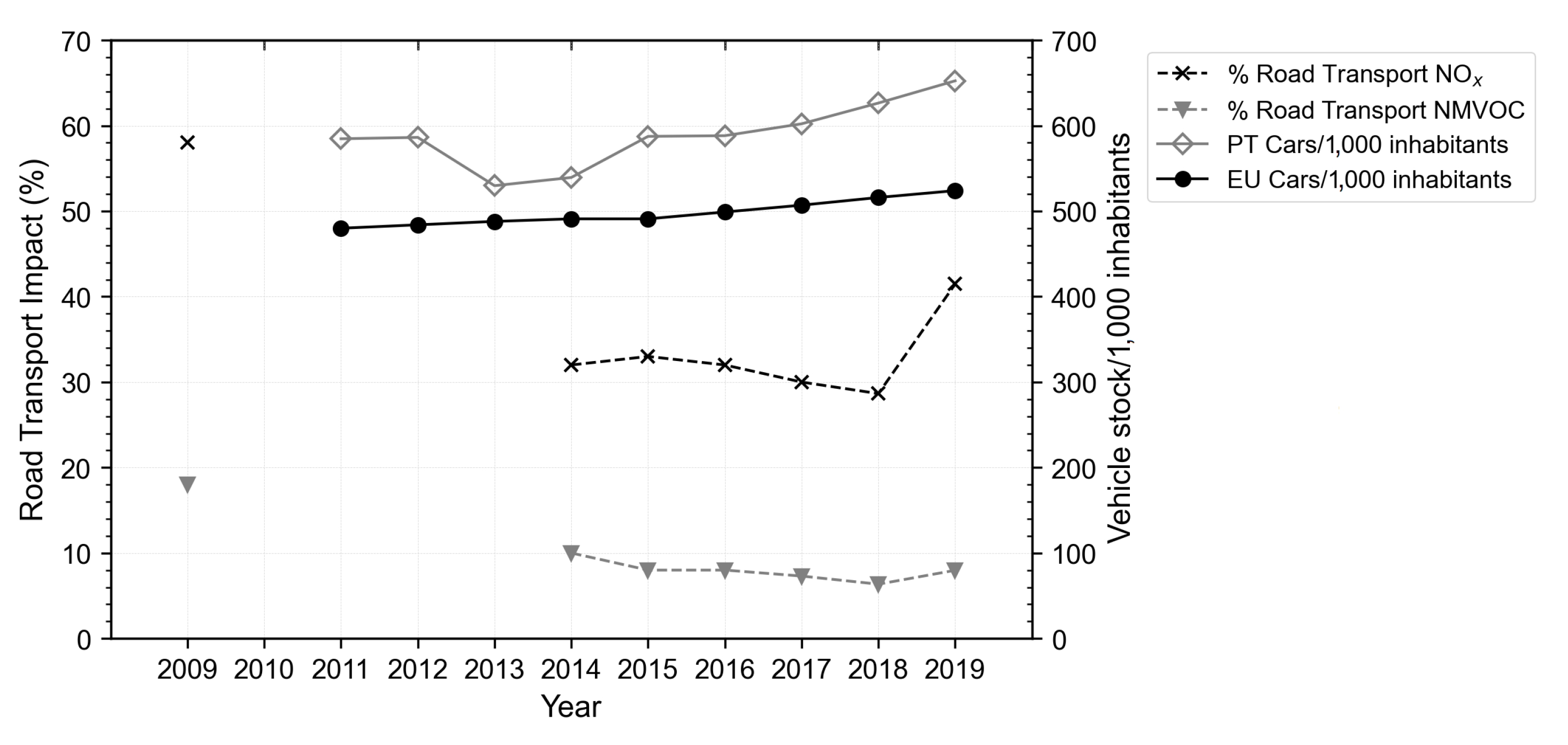
The road transportation sector is seen as one of the main contributors to the O${}_3$ precursors: NO${}_x$ (30%) and NMVOC (8%). In Europe, the estimated share of responsibility for the overall NO${}_x$ and NMVOC emissions level is depicted in Figure 1 alongside with car ownership (Europe and Portugal). We observe the overall increase of the Portuguese car stock from 8% in 2010 to 30% in 2018 but we should note that cars after 2014 have had stringiest NO${}_x$ emission limits (Euro5 and Euro6).

Since the Gothenburg Protocol in 1999 (Protocol to Abate Acidification, Eutrophication and Ground-level O${}_3$), the problem of ground-level O${}_3$ was recognized. The Air-Quality Directives 2008/50/EC and 2004/107/EC set legally binding limits for ground-level concentrations of outdoor air pollutants, including NO${}_2$ and O${}_3$.

In EU28, since 1990, emissions of both NO${}_x$ and NMVOCs decreased by 61% and 58% respectively. However, for O${}_3$, a secondary pollutant photochemically controlled, its mitigation is not as straightforward and despite the push for clean air in European cities, by means of the road vehicle emissions standards and the industrial facilities emissions limits, the O${}_3$ trend is not following the anthropogenic precursors trends. Some authors argue that the decrease in particle emissions may trigger higher radiation available for the photochemical reactions and thus increasing surface O${}_3$ formation [22]. Following the same logic, the observed increase in CO_2eq emissions would have the opposite effect, less solar energy available (light scattering) for the photochemical reaction which could potentially reduce O${}_3$. The effects of global radiation (GR) on ground-level O${}_3$ through the photochemical reaction have already been established in another work by the author [4]. Other studies have also established GR-O${}_3$ correlation, which ranges from 0.4 to 0.6 (R${}^2$) [23,24].

In recent years there has been a further NO${}_2$ reduction with the increase of EV adherence, such as pure electric battery electric vehicles (BEV) and plug-in hybrid electric vehicles (PHEV), and the application of European emission standards for road transport and internal combustion engine vehicles (ICEV).

EV adherence can affect pollutant dynamics and its influence on air quality is seen as beneficial due to the reduced, or nonexistent, combustion of fuel for these types of vehicles while circulating. Therefore, fleet electrification and the stringiest emission regulations, should contribute to the decrease of ground-level O${}_3$. However, this does not seem to be the case every time and evidence for these contradictions can be seen in the same study using the same model [25]. This study, conducted by Brinkman et al. 2010, highlights how in some cases there has been an overall decrease of 2–3 ppb O${}_3$ concentrations due to the projected penetration of PHEV vehicles, while in other instances large O${}_3$ increases were found in other areas. The last portion of these findings seems to be in accordance with other studies that find localized O${}_3$ increase [26]. It is also in line with the fact that despite EU legislation leading to improvements in air quality in 2018 and the crescent adherence to electric vehicles, 34% of citizens were still exposed to O${}_3$ above EU limit values (8-h 120 µg/m${}^3$) [27].

There are two possibilities to track ground-level O${}_3$ concentrations: either by satellite (e.g., TROPOMI Sentinel-5P) or by terrestrial air-quality monitoring stations (AQMS). In this research we examine terrestrial AQMS which are divided in Traffic, Background and Industrial AQMS. Traffic AQMS are placed in heavy traffic affluence urban roads with contiguous buildings. Background AQMS are placed in urban locations with noncontiguous buildings and green areas. Industrial AQMS are placed near industrial sites. According to the Portuguese Environmental Agency, background AQMS reflect the exposure of the general population to pollution in Lisbon. Surveys of background AQMS in different world locations [28] reveal that the annual O${}_3$ cycle at background sites in the Northern Hemisphere (NH) are characterized by spring maximums, peaking during the month of May. There is no consensus on the origin of the spring maximum. Modern day annual average background O${}_3$ concentrations over the mid-latitudes of the NH vary between approximately 20–45 parts per billion (ppb). Model projections using IPCC emission scenarios for the 21st century indicate that background O${}_3$ may rise to levels that would exceed internationally accepted environmental criteria for human health and the environment. Recent global chemical transport model studies indicate that pollution originated from Asia contributes about 3–10 ppb to background O${}_3$ levels in the western United States during the spring. A continued rise in anthropogenic emissions from Asia is expected to increase the background level even further. This reveals the intercontinental transport phenomena impact on ground-level ozone [29].

Regarding worldwide monitoring, the distribution of anthropogenic O${}_3$ precursor emissions generally correspond to regions with human habitation. Most NO${}_x$ emissions occur in the NH as previously stated [30]. Moreover, 30% of the present-day tropospheric O${}_3$ burden is attributable to human activity [31]. Cooper et al., 2014 [19], provided an overview of tropospheric O${}_3$ global distribution and trends based on more than 20 years of data (1990–2010). Using yearly average O${}_3$ values, it concluded that there is an increasing trend since 1970 in which O${}_3$ went from 20 ppb to almost 60 ppb in Europe, and from 30 to 60 ppb in North America. From 1950–1979 until 2000–2010, all available NH monitoring sites indicate increasing O${}_3$, with 11 out of 13 sites with statistically significant trends of 1–5 ppbv per decade. Qualitative O${}_3$ observations indicate that 19th century O${}_3$ concentrations most often peaked in spring with some peaks continuing into early summer. By the end of the 20th century O${}_3$ in NH had shifted to a summertime peak. However, the study mentions that some rural sites have shown seasonal peaks of O${}_3$ shifting back to spring due to a reduced summertime at northern mid-latitudes.

In Jerry R. Ziemke et al., 2019 [32], evidence from combined satellite measurements and a chemical transport model provide insights into tropospheric O${}_3$ over the last four decades (1979–2016). There is evidence that increases in O${}_3$ are global, yet highly regional due to the combined effects of regional pollution and transport. The total column of O${}_3$ has been increasing and extending in the NH region. Measurements have increased from +1.2 to +1.4 DU per decade (1979–2005) to about +3 DU per decade or greater (2005–2016) (1 DU ≡ 0.0214 $·$ t $·$ km^–2 for O₃).

Focusing on the European region, the European air-quality database AirBase allow us to depict the trend of O${}_3$ annual mean daily 8-h max concentrations for 2001–2010 per AQMS type (traffic, urban and rural) seen in Figure 2.

The traffic AQMS consistently registered the lowest values yet appears to be converging with urban and rural AQMS in the later years. Rural AQMS present the highest O${}_3$ concentrations while urban sits somewhere in the middle. It is worth noting that both our traffic AQMS and non-traffic AQMS are urban; however, they behave differently as it will be discussed with detail in the results section.

There is a health risk indicator proposal by the World Health Organization (WHO) called SOMO35. This proposal consists of the sum of O${}_3$ means over 35 ppb (70 µg/m${}^3$) [34]. For each day, the maximum of the daily 8-hour running average for O${}_3$ is selected and the values over 35 ppb are summed over the whole year. If we let Ad${}_8^{\mathrm{d}}$ denote the maximum 8 hourly average O${}_3$ on day d, during a year with Ny days (Ny = 365 or 366), then SOMO35 can be defined as:

$$\mathrm{SOMO}35\left({\displaystyle \frac{\mu \mathrm{g}}{{\mathrm{m}}^3·\mathrm{days}}}\right)=\sum _{\mathrm{d}=1}^{\mathrm{d}={\mathrm{N}}_{\mathrm{y}}}\max \left({\mathrm{Ad}}_8^{\mathrm{d}}-35\mathrm{ppb},0.0\right)$$

(7)

where the max function ensures that only Ad${}_8^{\mathrm{d}}$ values exceeding 35 ppb are included. The corresponding unit is ppb $·$ days or (µg/m${}^3$$·$ days). This indicator is a calculation based on combining terrestrial monitoring data at regional and urban background stations with results from the European Monitoring and Evaluation Program (EMEP), chemical transport model, and other supplementary data. In Figure 3 and Figure 4, we observe a non-monotonous trend with seemingly increasing peaks. The EU28 peaks are also not monotonous but contrarily to Portugal are decreasing in comparison with 2006. The estimated premature deaths due to tropospheric O${}_3$ agree with this indicator trend for the EU28 data but not for Portugal.

In 2016, according to the European Environmental Agency (EPA), the premature deaths in Portugal due to ground-level O${}_3$ were 18% higher than the EU28 average of 28 deaths per 1 million inhabitants. Changes in surface O${}_3$ are influenced by meteorological conditions and anthropogenic precursors, hence, changes due to NO${}_x$ precursor mitigation may be masked by the varying meteorology. In an author’s previous study there is evidence that O${}_3$ is not NO${}_x$ sensitive [4] in Portugal for the year 2017.

This paper seeks to justify ground-level O${}_3$ trends in the past decade in Portugal, to better foresee future trends. The city of Lisbon, Porto and Coimbra, seen Figure 5, are selected as case studies due to being in the top 10 places in Portugal with high road densities and population densities of 6446 inhabitants/km${}^2$, 5726 inhabitants/km${}^2$ and 449 inhabitants/km${}^2$ respectively, according to the latest 2011 Census. We have 8 years of AQMS data for ground-level O${}_3$, NO, NO${}_2$ and nearby weather stations (WS) measuring global radiation (GR), humidity and temperature in the period 2010–2018.

Our 10-year datasets of pollution and weather will allow us to observe daily, monthly and yearly trends, day-night cycles, weekday (WD) versus weekend (WE) trends, seasonality, and NO${}_2$, O${}_3$, NO and GR relationships. This will be useful to draw our own conclusions for Lisbon, Porto and Coimbra pollution trends and compare our values with known and consistent worldwide observed data regarding the weekend effect [4], seasonality and yearly trends.

We also make remarks about traffic flow of diesel vehicles and provide graphical computations that help explain how they create the perfect conditions for high NO concentrations which are then transformed in NO${}_2$ through the reaction in Equation (1). Modelling studies claim that if all Diesel vehicles were under the Euro 6 norm, there would be a general decrease in regional and urban NO${}_2$ concentration [16]. Similarly, other modelling studies argue that it would also lower O${}_3$ by up to 26% in urban areas [17]. Lastly, we summarize posing the questions that will be addressed in this research:

(a)

How do daily, monthly, and annual trends of NO${}_x$ and O${}_3$ for Lisbon, Porto and Coimbra compare?

(b)

Are these trends the same over all periods for all AQMS?

(c)

Are NO${}_2$ peaks coincident with NO peaks?

(d)

Is hourly O${}_3$ well correlated with global radiation (GR) and NO${}_x$ (NO${}_2$ + NO) emissions over the years?

(e)

How does the weekend effect compare with other studies? Does it present trends and seasonality?

(f)

Has O${}_3$ been increasing or decreasing throughout the years? How do traffic AQMS compare with non-traffic?

(g)

Can we relate NO${}_2$ and O${}_3$ with the number of vehicles, car stock (age and technology), European standards and fuel sales?

(h)

If so, how has traffic affected NO${}_2$ and O${}_3$ air pollution?

(i)

Can we infer EV influence?

2. Materials and Methods

To answer the proposed questions, datasets of pollution and weather data were provided by the Portuguese Institute for Sea and Atmosphere (IPMA) and the Portuguese Regional Coordination and Development Commission (CCDR) for the period 2010–2018. For AQMS data, all values were obtained through an open-source platform created by the Portuguese Environment Agency (APA) under the name of QualAr [20,21]. The QualAr website gathers its data from the air-quality monitoring network managed by the Regional Commission of Coordination and Development (CCDR) and under the responsibility of the Ministry of Environment. The whole Portuguese network is comprised of 63 AQMS spread throughout the country.

The AQMS in this research were selected based on measuring simultaneously the same pollutants and having the least amount of missing data for all the possible AQMS and regions selected. The map of Lisbon can be seen in Figure 6 while all AQMS coordinates on

Table 1. Parameters and type of monitoring stations in study. For geographical location of Lisbon AQMS see Figure 6.

Monitoring Station	Type	Parameters	Location (LAT, LON)
Entrecampos	Traffic (T)	O${}_3$, NO${}_2$, NO and NO${}_x$	38.7486, −9.1488
Beato	Background (NT)	O${}_3$, NO${}_2$, NO and NO${}_x$	38.7336, −9.1144
Restelo	Background (NT)	O${}_3$, NO${}_2$, NO and NO${}_x$	38.705, −9.2102
Escavadeira	Industrial (NT)	O${}_3$, NO${}_2$, NO and NO${}_x$	38.6586, −9.0669
Olivais	Background (NT)	O${}_3$, NO${}_2$, NO and NO${}_x$	38.7688, −9.1080
Porto	Background (NT)	O${}_3$, NO${}_2$, NO and NO${}_x$	41.1475, −8.6588
Coimbra	Background (NT)	O${}_3$, NO${}_2$, NO and NO${}_x$	40.2084, −8.4121
Gago Coutinho	Weather Station (WS)	GR	38.7661, −9.1284
Porto	Weather Station (WS)	GR	41.1844, −8.6444
Coimbra	Weather Station (WS)	GR	40.2134, −8.4551

. The data gathered from all stations, for Lisbon, Porto, and Coimbra, consist of a total of 3,155,520 million hourly measurements (N) with 2.7% of that data missing (N_miss). These measurements account for hourly NO${}_2$, O${}_3$, NO, and GR for 8 years for 10 stations (AQMS and WS). In the only instance where missing data from a dataset exceeds 25%, in the weekend effect by percentage analysis, this missing data is represented as a blank box for any given month/year. We should note that this graphical representation with some missing data points was necessary, as it represents the only Traffic AQMS that measures ground-level O${}_3$. This traffic AQMS is in Lisbon, near a traffic intersection in Entrecampos [4]. The other AQMS are either industrial or background and therefore classified as Non-Traffic (NT) in this research. For traffic and non-traffic comparisons, non-traffic AQMS data was concatenated as they have similar values and trends. The data is temporally homogeneous with a correlation of 0.90–0.98 between all AQMS (supplementary files). Concatenating data was done for two reasons: First it bridges data gaps of some of the background AQMS. Second, it makes practical and logical sense to better depict differences between traffic and non-traffic AQMS.

The WS data was provided by IPMA. This includes hourly global radiation (GR), temperature, humidity, and precipitation. From this weather data, GR was selected as indicative of hν in the photolysis reaction (4). Temperature is highly correlated with GR while precipitation was seen to have no impact on O${}_3$ levels [4]. In Figure 6 we highlight Lisbon AQMS and show their location geographically as well as its closest WS (red dot).

All hourly data is in the Greenwich Mean Time Zone. The parameters in study, geographic coordinates and the description of all monitoring stations can be seen in Table 1.

Data sets pertaining economic and car stock data were obtained through the Portuguese National Statistics Institute (INE) [36], PORDATA [37] and EUROSTAT [38]. This data includes unemployment and gross domestic product (GDP) as well as yearly car stock by age and technology. The urban mobility trend in Portugal was characterized in terms of vehicle technologies (ICEV, LPG, BEV, PHEV, and HEV), fuel technology (Diesel/Gasoline), and Euro standards.

Table 2. Economic data and EU emission standards.

Year	Unemployment	GDP	EU Emission Standards *
2010−2012	10.8−15.5 %	−6 %	Euro 5 & Euro 5a
2013−2014	16.2−13.9 %	+2 %	Euro 5b, Euro VI & Euro 6
2015−2018	12.4−7.0 %	+14 %	$--$

* The EU emission standards dates represent the moment they were applied to all models.

summarizes economic and emission standards data and Figure 7 shows the car and bus stock versus GDP. Knowing that the Portuguese population has remained roughly the same from 2010–2018 (10 million), we can observe that car stock decreases in 2012 and only recovers to pre-2012 levels in 2014. Bus adherence decreased from 2010 until 2014. It started recovering in 2015 but remains distant from 2010 numbers. Overall passenger car stock is well correlated with GDP.

It should also be noted that in car stock and fuel sales comparisons we use country-based data due to either not having city-to-city-based data, or because their trends are nearly identical. Portugal is a relatively small country where Porto, Coimbra and Lisbon account for nearly 50% of all population and this its indirect correlation.

The most relevant source of air pollution is the combustion products resulting from the LPG, gasoline, and diesel burning in combustion engines (present in the ICEV, LPG, PHEV and HEV technologies). Looking at Figure 8, the fuel sales consumption goes into a downward trend from 2010 until 2014. This coincides with economic recession periods felt all over the world but especially in Europe due to the post-housing bubble in the USA [39]. This is in accordance with Table 2, where it can be seen that in Portugal, the harshest part of the recession period was around 2012–2013, when unemployment increased from 15.5 to 16.2% and GDP dropped 6%. Although in the results section we make city-to-city-based comparisons, we still used country-based car stock and fuel sales data due to either not having city-based data or, in the case of fuel sales, they displayed nearly identical trends at a country level and city-level as seen in the supplementary files. This is mainly because Lisbon, Porto, and Coimbra account for nearly 50% of the Portuguese population and have considerable weight over the overall data.

Diesel fuel has a huge expression in final energy consumption for road transport (passenger cars, passenger bus, and goods transport), which seems correlated with fuel sales. In addition to this, if we also consider car stock age, seen in Figure 9, we can argue that both the economic factors and fuel sales contribute to higher or lower levels of combustion products. This is apparent in Figure 8. When fuel sales drop from 2010 until 2013, we see a decrease of NO${}_2$ in the traffic AQMS accompanied by a sharp O${}_3$ increase in maximum values. This is in fact the highest value of annual mean O${}_3$ using daily 8-h maximums that was achieved from 2010–2018.

Therefore, to reflect urban mobility levels on ground-level O${}_3$ trends, the indicator total fuel sales for road transport will be taken into consideration.

Additionally, we recall that the adherence to EVs has risen in recent times; however, despite increasing 680% from 2012 to 2018, this value is still orders of magnitude lower than the Gasoline and Diesel cars circulating. Therefore, it is unlikely that it has played an important role in air pollutant dynamics from 2010–2018.

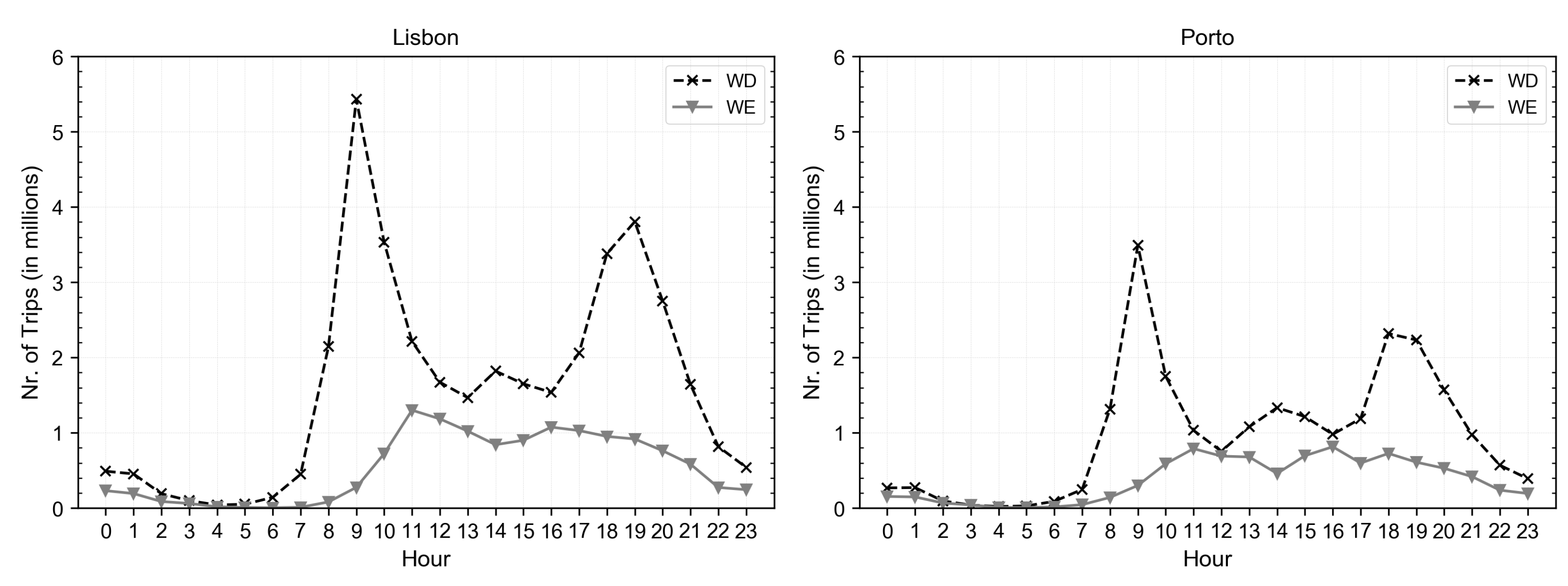
A recent survey by INE has gathered mobility patterns in Portugal for 2017. This survey infers that the number of trips in both weekdays and weekends is mainly made by car (67.6% in Porto and 58.9% in Lisbon). In the weekdays, the main purpose of these trips is commuting to work. In the weekends, it is for shopping. The distribution of the number of trips along the day for Lisbon and Porto is depicted for both weekdays (WD) and weekends (WE) in Figure 10. The trip corresponding “hour” represents the time of arrival at the destination, which means that actual on-road peaks happen early on. Considering average commuting times, the lag could be between 30 to 45 min. This will allow us to cross NO${}_x$ traffic AQMS with typical daily cycle traffic flows (trips). Thus, trips will serve as another indicator of urban mobility used to reflect NO${}_x$ emissions throughout the day in both WE and WE. It has been proved that the majority of tailpipe NO${}_x$ emissions are in fact NO [40], which by means of Equation (1) reaction, form NO${}_2$.

To research trends in ground-level O${}_3$ in terms of WD versus WE and determine the weekend effect, the following metric proposed in the authors previous work [4] will be used:

$$\mathrm{weekend}\mathrm{effect}{\mathrm{O}}_3 (\%) =\left({\displaystyle \frac{{\mathrm{Weekend}}_{\mathrm{peak}}-{\mathrm{Weekday}}_{\mathrm{peak}}}{{\mathrm{Weekend}}_{\mathrm{peak}}}}\right)\times 100$$

(8)

In Equation (8), we calculate the percentage by which the weekend effect has increased or decreased from weekday to weekend. To make use of this equation, we first find peak daily O${}_3$ concentrations. In other words, we calculate the maximum daily O${}_3$ concentrations for each day, in our case in ppb, and then monthly average these values for both weekend and weekday. These monthly values are then plugged into Equation (8) giving us the corresponding weekend effect percentage, which can be positive or negative. A positive weekend effect means that O${}_3$ concentrations were generally higher on weekends than on weekdays. A negative weekend effect means the opposite and that we did not observe the weekend effect.

Afterwards, to further our understanding of NO${}_x$-O${}_3$ relationship and how that might possibly relate with VOCs, we applied a similar methodology to Song et al. 2011 [41] which compares averaged daily concentrations of O${}_3$ versus NO${}_x$. We use this methodology to then compare traffic versus non-traffic AQMS and comment on NO${}_x$ sensitivity.

To finish our methodology section, we remark that unfortunately there is only one traffic related AQMS that is in Lisbon as seen in Figure 6 or Table 1. Nevertheless, for Lisbon, it will be possible to assess the differences between traffic and non-traffic AQMS. It is our objective to make comments recognizing weekend effect seasonality and its progression over the years. Despite not having traffic AQMS for Porto and Coimbra, these non-traffic (background) AQMS will be used for hourly and monthly weekend effect comparisons between all stations.

All the historical data is in a supplementary file. The Python file to manage the data (alpha version), is also available in the supplementary files.

It should be stated that for the 8-hour daily max calculations, we used the methodology stated by Directive 92/72/EEC. It assigns three 8-hour periods to each day. The first period starts in the first day of measurements at 17 h (so the period 17–1 h is the first 8-h period of a day followed by 1–9 h and 9–17 h) [42]. Then, the max daily value is selected and annual averaged. The remaining calculations are straightforward and include means and maximums. This can be searched in the Python code. When some different data interpretation is made in this paper, as seen in WD and WE, it is explained or referred to Equation (8).

3. Results

In this section, we present hourly, daily, monthly and annual trend data for NO${}_2$, NO, O${}_3$, and GR for 10 stations (7 AQMS + 3 WS). Of these stations, 6 are in Lisbon, 2 in Porto and 2 in Coimbra. This means that every region has at least 1 AQMS and 1 WS. There is only one traffic AQMS type which is in Lisbon, the rest were considered non-traffic. In graphical representations it will often be seen traffic as “(T)” and non-traffic as “(NT)”. We joined the Industrial AQMS with the background AQMS as it was found that they represent the same trend, amplitude of values and overall concentrations as the background stations. We also note that since there were no traffic AQMS in Porto or Coimbra, some graphical presentations were only made for Lisbon, as it will be stated in the corresponding Figure legends. Usually, these Lisbon representations happen when comparing traffic versus non-traffic since Porto and Coimbra do not have traffic AQMS.

The order of presentation will start with hourly trends and work towards daily (with statistical analysis), monthly, yearly, seasonal, weekend effect (WD versus WE), and end with a general view and comments on the data.

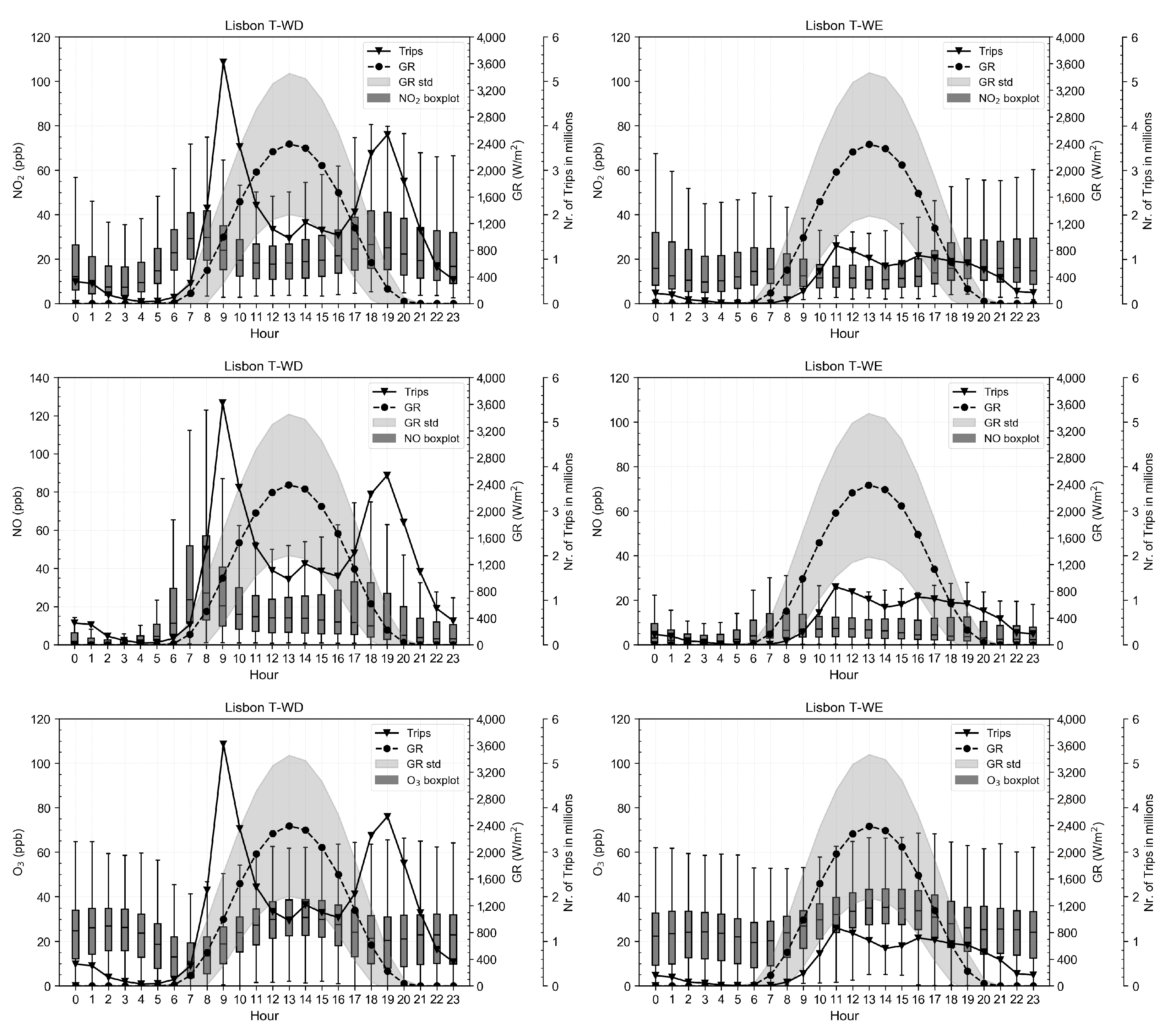
To better understand daily trends of NO${}_2$ and O${}_3$, we crossed the number of trips by hour mentioned in Figure 10, with NO${}_2$, GR, and O${}_3$. We also compared traffic, non-traffic, WD and WE. We should see clear differences between the most active parts of the day/week and pollutant peaks. We should not forget that the hour in the trip metric represents the arrival at the destination. This explains the lag of 30 to 45 min from pollutant peak concentrations to trip peaks.

In Figure 11, there is a clear hourly trend for all pollutants. During the night from 2 to 4 h, on the periods of least activity, the lowest median values for NO and NO${}_2$ are observed. This happens for Coimbra and Porto as well (see supplementary graphics).

In the morning, from 6 until 8 h there is a significant increase in NO${}_2$ and NO. This coincides with the trips taken by the population data seen in Figure 10.

Lisbon traffic AQMS presents the highest concentrations of NO and NO${}_2$. For NO${}_2$ in the traffic AQMS, the maximum absolute value reached is 80 ppb. This happens during WD at 8 h. The complexity of predicting O${}_3$ resides in its interactions with other gases, such as NO${}_2$ and NO, but as well as its interaction with GR. As NO${}_2$ production subsides, the increase in GR throughout the 12–16 h provokes production and accumulation of O${}_3$ through reaction Equations (1), (4) and (6). These processes cause the peaks seen in the figure. These concentrations can become consistently high during periods of high GR as shown in the figure. Still referring to the traffic AQMS in Figure 11, we can attest that the O${}_3$ cycle presents a clear trend over all years of data and has a correlation with GR. There is also a correlation between emissions of NO${}_2$, NO, and trips which are all coincident in time. These visual affirmations are confirmed by the statistical analysis in

Table 3. Pearson correlation table for all AQMS data (N = 424,891).

Variables	1.	2.	3.	4.
1. NO${}_2$	—
2. NO	0.64	—
3. O${}_3$	−0.52	−0.37	—
4. GR	−0.19	−0.06	0.45	—

. Differences between WD and WE are not obvious but will be researched in more detail later. Porto AQMS despite being a non-traffic AQMS, displays similar behaviors to Lisbon traffic AQMS (supplementary graphics).

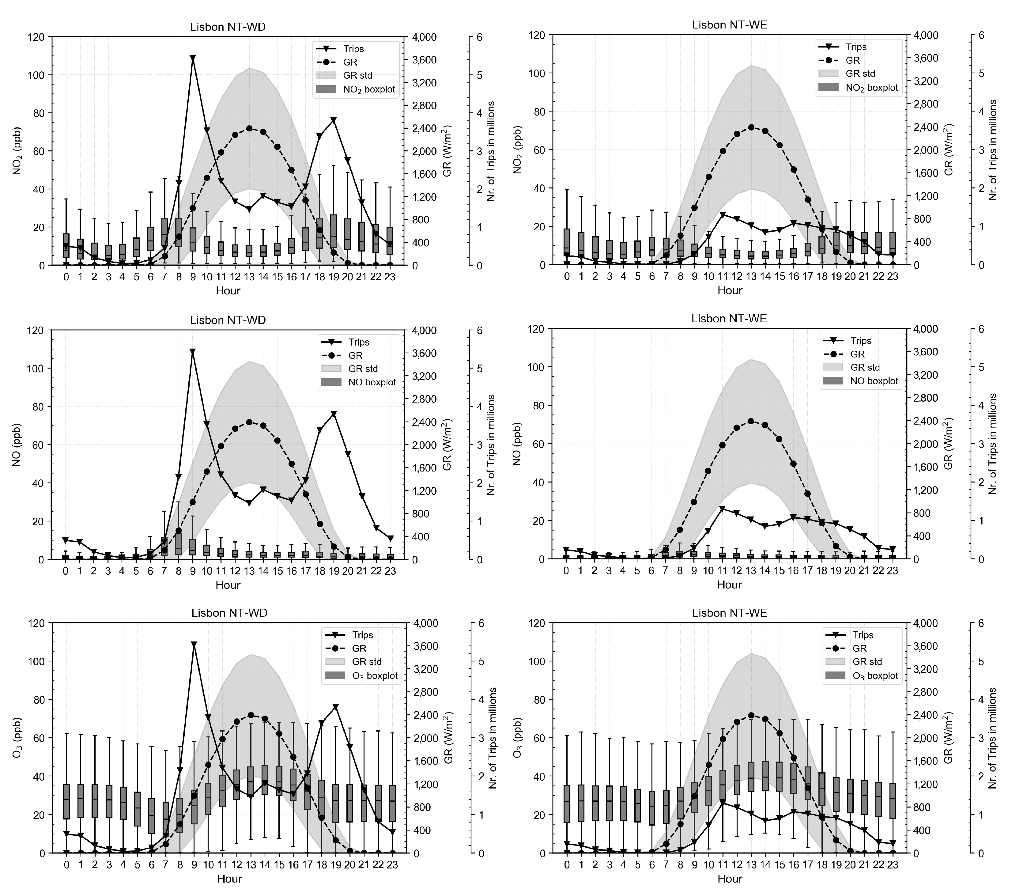
Next, we do the same analysis but for Lisbon non-traffic AQMS. It is expected that we have smaller NO${}_2$ and NO peaks as these AQMS are not right next to high intensity traffic roads. Looking at Figure 12, we can effectively verify that the peaks of NO${}_2$ and NO present lower overall values; however, O${}_3$ has increased. For the non-traffic AQMS the maximum NO${}_2$ registered value is of 46.8 ppb, a difference of 33.2 ppb versus the traffic AQMS. Both the lowest NO${}_2$ peak hour and highest O${}_3$ peak hour happen on the non-traffic AQMS during WE. The non-traffic AQMS during WE has roughly 5 ppb higher maximums in peak hours than during WD. Coimbra has a similar behavior to non-traffic AQMS with the lowest NO${}_2$ maximum of 35 ppb registered and the highest O${}_3$ maximum of 70 ppb. Our values and trends are in accordance with the values in Turia river basin [43] which observed that AQMS further away from traffic registered lower concentrations of NO${}_2$ than AQMS closer to the city and vice versa for O${}_3$. In Nuria Castell-Balaguer et al. 2012 [43] the argument that breeze plays a role in carrying O${}_3$ pollution along with primary pollutants is made. We understand this statement arises from peak delays of NO${}_2$ from traffic AQMS to non-traffic AQMS which implies that pollutants were carried to locations with no traffic emissions sources. However, we do not observe these peak shifts which leads us to lean towards the remarks made in F. Ahamad et al. 2014 [44]. It states that local influence of traffic is the main pollutant variation culprit. This does not mean that air transport does not play a role, as other studies have shown [45].

We have therefore established that clear daily trends are verifiable over all the years in study from 2010 until 2018, for Lisbon, Porto and Coimbra. There is also a good indication that combustion emissions from road transport are a major contributor to the daily trend cycles.

A more complete representation of all AQMS was computed in Figure 13. It shows how all AQMS compare with each other, including Porto and Coimbra non-traffic AQMS. From the figure, we can see the same trends for all stations, similar to what is shown in Figure 11 and Figure 12.

To elaborate on air mass transport and road emissions as stated previously, we investigate Olivais and Porto behavior seen in the Figure 13. We can see that Olivais has considerably higher NO${}_2$ peaks for a non-traffic AQMS. These peaks also seem to hold on high concentrations for longer than other AQMS. Porto also displays this pattern. There may be some air mass transport effect as both Porto and Olivais AQMS are situated south-east of major pollutant sources. Porto AQMS is downwind from Porto city and Olivais AQMS is downwind from Lisbon airport. As NO${}_x$ increases, so does the titration of O${}_3$. This would explain why these AQMS O${}_3$ concentrations are lower than expected for non-traffic AQMS. It is also worthy of note that some of these city-to-city differences, such as non-traffic Coimbra and Porto having generally lower O${}_3$ and NO${}_2$ than traffic Entrecampos, can potentially be explained by the differences in peak radiation as Porto and Coimbra have relatively less average radiation than Lisbon due to their geographic location.

It would be interesting in future analysis to include data from SARS-CoV-2 outbreak periods, which include the airport shutdown, and see if this is verifiable. It would also be interesting to see how weekend lockdowns have affected WD and WE relationship as every AQMS shows an increase of O${}_3$ during the weekend due to less NO${}_2$ and NO emissions (further corroborated in Figure 16).

Still in Figure 13, similar to what is seen in Nuria Castell-Balaguer et al. 2012 and other studies [44,46], O${}_3$ hourly maximums are achieved at 13–15 h, meaning they occur 1 to 3 h after solar peak. This is in accordance with GR having a pivotal role in O${}_3$ formation. Therefore, GR appears to be a good indicator for daily O${}_3$ variations. To verify this statement, a statistical analysis (Pearson correlation) was conducted and can be seen in Table 3. All the data presented is congruent in time, meaning that if a value is missing for any given hour for a certain variable, the whole hour for all variables is discarded. Thus, from Table 3, we observe that for all the data in study, GR-O${}_3$ presents a correlation coefficient of 0.45. This value is in line with the 0.4 to 0.6 range cited in other works [23,25]. Succinctly, this means that up to 45% of O${}_3$ variation in Portugal can be attributed to GR. We can also confirm all the visual observations and correlations of NO, NO${}_2$ and O${}_3$ in Figure 11 and Figure 12.

Still on the topic of correlations and applying Song et al. 2011 method [41], Figure 14 show us the negatively correlated averaged daily NO${}_x$-O${}_3$ plots for both traffic and non-traffic AQMS, as well as the quadratic equation that best fits the data.

In Figure 14, both the traffic and non-traffic AQMS present similar quadratic equations. We also sub-divided this correlation into several periods, such as WD vs. WE and economic recession vs. economic recovery, seen in the supplementary files, but found no meaningful differences when compared with the overall 2010–2018 figure trends. The implications in NO${}_x$ sensitivity and the theoretical basis for this analysis is best quoted by Hashim et al. 2021, taken from Seinfeld et al. 2006 [8,11]. It tells us that while instantaneous reaction dynamics during the day affect the production rate of O${}_3$, the correlations between averaged NO${}_x$ and O${}_3$ concentrations over the years reflect the mixed effects of chemical reactions, transport patterns, atmospheric dispersion, etc. Therefore, in Figure 14, we can observe that throughout the 8 years of plotted data, there has been a consistent negative correlation between NO${}_x$ and O${}_3$, which points toward Lisbon possibly not being sensitive to NO${}_x$, but sensitive to VOC instead. We reiterate that to make more concise arguments, we would need more VOC data which is not sufficiently available for the 8-year historical analysis comparison. Hopefully, going forward, with the increase of data availability from the crescent adoption of low-cost sensors, as stated by the author in another work [47], we can see these data availability flaws fixed. Nonetheless, we can still suggest with good grounds the possibility that Lisbon was VOC–sensitive from 2010–2018, but recognize more research is needed [11,48].

We have sub-divided this correlation into several periods, such as WD vs. WE, economic recession vs. economic recovery, but found no meaningful difference pertaining to its NOx sensitivity.

Moving from daily data to monthly data, we present an analysis of all stations in Figure 15. Monthly data exhibits seasonality trends for all stations. When comparing the pollutants with each other we notice from Figure 13 how the GR, O${}_3$ and NO${}_2$ mean peaks do not align in a similar or inverse relationship. Instead, we notice that the O${}_3$ peaks occur as GR increases but start to descend when maximum GR is reached. Furthermore, looking at Figure 13, O${}_3$ peaks seem to be in accordance with Cooper et al. 2014 [19] which states that western Europe typically experiences a springtime peak (May). Regardless, it does appear that Porto and Coimbra peak one month earlier to all the remaining AQMS. Several elements could be at play here as the locations topography and latitude are different. Coimbra and Porto do have lower GR than Lisbon, but how much of a role it plays in this early springtime peak could not be ascertained.

Coimbra and Porto register mean concentration peaks of 31.9 and 30.6 ppb in April while the remaining AQMS register their peaks in May. Escavadeira registered the highest monthly mean peak of 39.3 ppb. These values are in line with other studies [28].

In Portugal, periods of high GR typically occur between May and August (spring-summer). The lowest mean NO${}_2$ values registered happen in July for all AQMS except Entrecampos (August), yet the highest mean O${}_3$ concentrations give place in May for most AQMS. What we are trying to hint at, is the seeming disconnect between O${}_3$ and NO${}_2$ peaks in monthly trends, they are still negatively correlated but their monthly peaks diverge. This can be explained through urban mobility indicators. We stress how mobility trends play a contributing role to air pollutant dynamics. The months of July and August are often associated with vacation time or school break period in Portugal. Thus, we register the lowest NO${}_2$ concentrations during summertime as the circulating vehicle stock decreases considerably [47]. During the winter, as everyone is back from vacation and GR values start decreasing, we see the highest mean peaks of NO${}_2$. It can be inferred that circulating car stock has a major impact in NO and NO${}_2$ emissions and consequently, through Equations (4) and (6), impact O${}_3$ formation.

Moving from monthly data to yearly trends and returning to the briefly mentioned subject of weekend effect seasonality, we wanted to understand how it has progressed over the years, and how traffic and non-traffic compare. For this, we elaborated the heatmaps seen in Figure 16. These O${}_3$ heatmaps show us the percentage of weekend effect on any given year and month in study. This percentage is calculated according to Equation (8) as previously explained. Positive percentages mean that concentrations of O${}_3$ on the WE were higher than concentrations of O${}_3$ on WD. This means that if we have a red box in any given month of the year, on average that month registered the weekend effect. Negative percentages (blue boxes) mean the opposite, no weekend effect. White blocks mean that more than 25% of data is missing, and the month was discarded.

We retain from Figure 16 that the weekend effect is more dominant in the traffic AQMS than in the non-traffic AQMS. The non-traffic AQMS are more balanced but still present a majority of weekend effect. There appears to exist some seasonality but to confirm this is the case, we consider

Table 4. Seasonal averages (%) for all AQMS.

AQMS	Spring (%)	Summer (%)	Autumn (%)	Winter (%)
Lisbon T	2.2	6.1	6.7	4.7
Lisbon NT	0.3	6.4	3.6	5.2
Porto NT	7.1	6.8	6.7	7.3
Coimbra NT	5.3	5.2	5.5	7.0

.

Porto and Coimbra, despite having relatively high spring and summer percentages, reach their highest weekend effect averages in winter, but do not seem to display any significant seasonality. The most notable seasonality trend happens for both traffic and non-traffic AQMS in Lisbon, which have their relatively lowest weekend effect percentage in the spring. We remind that looking at Figure 15, spring is when we achieve peak O${}_3$ means in all AQMS. However, Porto and Coimbra, which have similar monthly mean trends, do not manifest this behavior.

When analyzing yearly weekend effect trends we notice that Lisbon also has a different behavior to Coimbra and Porto. Lisbon seems to follow the fuel sales indicator more closely than Coimbra and Porto, as seen in Figure 8. The global period of 2010–2018 also acts in accordance with the same upward trend of car stock data in Figure 9. It is a possibility that Lisbon traffic AQMS not only felt the economic crash the soonest (2011–2012), as it might have recovered faster too. Still for Lisbon AQMS, the weekend effect was highly intensified afterwards, in 2014 and 2015, showing the highest monthly differential of 41.5% between WD and WE peaks in October. Afterwards, in 2016, 2017, and 2018, August presents the most consistent weekend effect with 24.5, 31.9 and 26.9% O${}_3$ increase from WD to WE. Regardless of the yearly differences, the global upwards trend for 2010–2018 is verified for all AQMS, starting with less weekend effect in 2010 and ending with relative higher percentages in 2018, as seen in Figure 17.

To summarize this weekend effect section, only the traffic AQMS follows both the increasing global trends of O${}_3$ concentrations (Figure 18) and increasing weekend effect (Figure 17) over the 2010–2018 period. This is in line with several other studies [49]. Porto and Coimbra have discrepancies that do not allow us to make the same claim. Once again, these can have many causes, different urban mobility indicators, different topology, different latitudes, etc.

To compare our percentage weekend effect results with other studies, the same metric would have to be used. The most commonly used metric was proposed by Altshuler et al., 1995 [6]. This metric takes into account the percentage difference between Wednesday (weekday) and Sunday (weekend); however, we consider that this metric is limited and possibly outdated. Regardless, according to Altshuler metric, we considered the summer months only. Through their metric, for the traffic AQMS (2010–2018), we obtain an average weekend effect of 28%. Using our metric, we register 11.6%. Considering the 28% results, it would seem that we have a similar weekend effect to Arizona [50].

The authors argue that while situations such as economic recessions or pandemic outbreaks provoke a decrease in NO${}_x$ and increase O${}_3$, they also seem to suppress the weekend effect in Lisbon but not in Porto or Coimbra. This is odd considering that the weekend effect has been theorized to have a correlation with the weekly pattern of traffic flow [5] and would be expected to have similar behavior with a yearly decrease of the traffic flow (NO${}_x$ emissions), but this was not the case for all AQMS. Further research into the weekend effect considering more economic data, urban mobility indicators and VOCs is required.

Moving from monthly data to yearly trends, we reproduced Figure 2 but for Portugal. We also added fuel sales and NO${}_2$ 1-h daily max concentrations for ease of interpretation. We apply the same 8-hour daily max for O${}_3$ annual mean calculations, as specified by EEA (European Environment Agency) [42]. The result can be seen in Figure 18.

If we compare Figure 18 with Figure 2, the similarity between the European and Portuguese trend for O${}_3$ annual mean is striking despite the 10-year difference. In both figures trend lines appear to be converging towards each other and have a set of sharp peaks. We do not elaborate as to why the 2003 O${}_3$ sharp peak happened in Figure 2 but it could possibly be connected to the 2000 financial crisis. We draw this parallel because an economic recession is most likely the culprit for Lisbon O${}_3$ peak of 39.3 ppb annual mean in 2013 seen in Figure 18 just as it is possible that the economic crisis of 2000 was the culprit of the European O${}_3$ annual mean peak of 42.5 ppb in 2003. We make this economic connection for Portugal based on the established relationship of vehicle stock and GDP, seen in Figure 7, and GDP and fuel sales, seen in Figure 8. Thus, the vehicle stock shows a sharp drop which is correlated with fuel sales, and so, we are expected to see a decrease in NO${}_2$, which we do. This sharp and continuous NO${}_2$ decrease caused by decreasing fuel sales might have caused the 2013 O${}_3$ peak. After 2013, NO${}_2$ is also well correlated with the number of total vehicles and car stock seen in Figure 7 and Figure 9.

There have been global efforts to balance the increasing vehicle circulation through mitigation measures which have effectively helped reduce possible NO${}_x$ as cited in David C. Carslaw et al. 2019. These measures include Euro 6, which was put in place in 2014 limiting NO₂ emissions at the tailpipe from 0.18 to 0.06 ppb. This is especially important considering the road transport industry impact depicted in Figure 1. However, for Portugal, these do not seem able to counteract both the increasing car stock and the aging car stock which went from 7.2 in 2010 to 12.7 years in 2019 [36]. In other words, this reveals that a lot of circulating diesel vehicles in Portugal do not comply with Euro 5 and 6 emission standards.

It has been shown in F. Zhao et al. 2020 [51] that critical events such as the SARS-CoV-2 outbreak cause sharp reductions of NO${}_x$ emissions. Even if we were able to achieve full mitigation similar to these critical events, F. Zhao et al. 2020 states that this decrease took no role on the mitigation of O${}_3$ pollution, but even caused the increase of O${}_3$ concentration as corroborated by Bauwens et al. 2020 [10].

Thus, we have established that much like the SARS-CoV-2 outbreak, critical events such as economic recessions take their toll in fuel sales and total circulating stock. We make the argument that as shown by Portuguese pollutant trend data, NO${}_2$ clearly decreases from traffic to non-traffic AQMS, from weekday to weekend, and even from school period to school break (winter to summer). Meanwhile O${}_3$ often increases during these periods, so it is hypothesized that if we were to achieve full mitigation tomorrow (including road transport), or if the fleet became all electric (100% EV), it is possible that unprecedented high O${}_3$ concentrations could be observed.

4. Conclusions

The aim of this work was to historically review Lisbon, Porto and Coimbra and observe daily, monthly and yearly trends as well as assess seasonality and relationships between all pollutants. We also investigated WD and WE as well as compare different types of AQMS. The results obtained have allowed us to make certain connections with urban mobility indicators and economy (car stock and fuel sales) which will be summarized when answering the proposed research questions:

(a)

How do daily, monthly, and annual trends of NO${}_x$ and O${}_3$ for Lisbon, Porto and Coimbra compare?

(b)

Are these trends the same over all periods for all AQMS?

(c)

Are NO${}_2$ peaks coincident with NO peaks?

(d)

Is hourly O${}_3$ well correlated with global radiation (GR) and NO${}_x$ (NO${}_2$ + NO) emissions over the years?

(e)

How does the weekend effect compare with other studies? Does it present trends and seasonality?

(f)

Has O${}_3$ been increasing or decreasing throughout the years? How do traffic AQMS compare with non-traffic?

(g)

Can we relate NO${}_2$ and O${}_3$ with the number of vehicles, car stock (age and technology), European standards and fuel sales?

(h)

If so, how has traffic affected NO${}_2$ and O${}_3$ air pollution?

(i)

Can we infer EV influence?

Our answers are as follows:

(a)

Daily trends are similar between all AQMS. During WD, NO${}_2$ median peaks occur at 8 h and O${}_3$ medians peak at 13–15 h. During WE, NO${}_2$ median peaks occur at 7 h instead, and O${}_3$ medians peak at 13–15 h as well. These O${}_3$ peaks occur 1 to 3 h after GR peaks. Monthly trends show how all AQMS have spring mean peaks; however, it is during summertime that the absolute maximums are reached. Yearly trends are similar for all AQMS with differences only in absolute values. The traffic AQMS of Entrecampos is the most NO${}_2$ polluted while Coimbra is the least. Inversely, the Lisbon traffic AQMS is the least O${}_3$ polluted while Escavadeira and Coimbra are the most. Their mean values reside between 30–45 ppb which is in line with other studies [28].

(b)

No, while overall yearly trends are similar, there are some differences for certain periods. Coimbra and Porto consistently have mean O${}_3$ spring peaks 1 month earlier than all the remaining AQMS (Lisbon). Over the years, trends for NO${}_2$ and O${}_3$ show better correlation during the economic events of 2011–2013 than the remaining years. More indicators and further research is needed to understand why.

(c)

NO${}_2$ and NO peaks are coincident in time for all AQMS. They are also correlated with urban mobility indicators such as trips seen in Figure 10.

(d)

O${}_3$ is well correlated with hourly NO${}_2$ emissions and GR, yet there are some peak delays in relation to each other. Factors such as air mass transporting and other non-accounted pollutants may play a role in these dynamics. There is also indication that both the Lisbon traffic and non-traffic AQMS are not NO${}_x$ sensitive but possibly VOC–sensitive over the years. Non-traffic AQMS is possibly more VOC–sensitive than the traffic AQMS due to a higher negative correlation of NO${}_x$-O${}_3$. In other words, average O${}_3$ concentrations exponentially increase as NO${}_x$ decreases.

(e)

Weekend effect is in line with other studies and would be comparable with Arizona, using Altshuler et al., 1995 [6] metric. However, using our metric, we noted that Lisbon has a very low spring weekend effect. The same cannot be said for Porto and Coimbra which present no significant monthly seasonality and remain relatively stable throughout the year. Despite this, a case can still be made about weekend effect trends being correlated with urban mobility indicators. From Figure 17, it is possible that Lisbon AQMS felt the economic impact sooner than Coimbra and Porto or in a higher capacity and should be further investigated. Regarding the whole 2010–2018 period, the weekend effect is trending upwards. Using our metric for the relatively stable 2015–2018 period, we have the following weekend effect percentages: Lisbon traffic (11.7%), Lisbon non-traffic (5.8%), Porto (8.4%) and Coimbra (7.6%).

(f)

For the Lisbon traffic AQMS 8-hour daily max concentrations, O${}_3$ has remained relatively stable going from 31.2 ppb in 2010 to 31.7 in 2018. The same relatively stable trends were verified for the background and industrial AQMS (non-traffic) but with higher values, respectively ranging from 34.8 and 36 ppb in 2010 to 33.4 and 35 ppb in 2018. Our data is in line with what has been registered from 2000 until 2010 in Europe as seen in Figure 2. The main difference is that Portugal has shown slightly higher concentrations of O${}_3$ than what was observed in the past in Europe. For a direct comparison we look at the traffic AQMS, overall, the Portuguese values fluctuate between 28–35 ppb while past traffic European measurements range between 27–31 ppb [33].

(g)

We observe global yearly trends using car stock, fuel sales and GDP, seen in Figure 8 and Figure 9. Lisbon seems to follow these trends more closely while Porto and Coimbra have an apparent 1–2 years delay. We do not know what has caused this apparent 1–2 years peak delay, more research is needed. At smaller scales (days and months), besides the trip indicator, most other indicators in the research cannot be used to understand NO${}_2$ and O${}_3$ relationship.

(h)

We can make claims, verified by other researchers [16,40], that reductions in car stock or emission mitigation can reduce NO${}_2$ which in turn can increase O${}_3$ [44,51]. Our data indicates this is also the case for Portugal.

(i)

Although it is unlikely that so far EVs have played any major role in mitigating NO${}_x$, we can infer that an exponential increase in EV car stock can alter current NO${}_2$-O${}_3$ balance and trends. Also, as we continue to renew the car stock and acquire more Euro 6 vehicles, we can potentially have this counteracted effect of lowering NO${}_x$ but increasing O${}_3$ concentrations over the coming years [40].

Our closing statements are that it is impossible to disconnect air pollution from their emission sources. These emission sources are part of a set of factors (economy, car stock, and fuel sales) which are an important part of urban mobility indicators. Emission mitigation also plays a role and while some authors have argued that absolute NO${}_x$ and NO${}_2$ emitted by most Euro 6 vehicles have decreased substantially, reducing the importance of NO${}_x$, we are inclined to disagree. With side effects such as O${}_3$ increase, it appears that NO${}_x$ has regained importance. More research using urban mobility indicators, VOCs, wind data, and more AQMS and year coverage is necessary to truly understand O${}_3$, NO and NO${}_2$ relationships over the years. From what was established in this research relating to critical events, meaning the reduction of NO${}_x$ but consequent increase in O${}_3$ concentrations, it is plausible that in a future scenario where mitigation is aggressively achieved, through emission standards and/or a shift of car stock to full EV, an unprecedented increase in O${}_3$ concentrations might take place.