Time Series Analysis of Evaporation Duct Height over South China Sea: A Stochastic Modeling Approach

Abstract

The evaporation duct could significantly affect the work status of maritime microwave communication systems in the South China Sea. Therefore, the exact forecasting of the evaporation duct is vital for the normal operation of the systems. This study presents a stochastic modeling approach to predict the future trends of the evaporation duct over the South China Sea. The autoregressive integrated moving average (ARIMA) model has been used for modeling the monthly evaporation duct height estimated from the Climate Forecast System Reanalysis dataset released by the National Centers for Environment Prediction. The long-term evaporation duct height data were collected for a period of 10 years from 2008 to 2017. The analysis of correlation function reveals the existence of seasonality in the time series. Therefore, a seasonal ARIMA model with the form as ARIMA (0,0,1) × (0,1,2)${}_{12}$ is proposed by fitting the monthly data optimally. The fitted model is further used to forecast the evaporation duct variation for the year 2018 at 95% level of confidence, and high-accuracy results are obtained. Our study demonstrates the feasibility of the proposed stochastic modeling technique to predict the future variations of the evaporation duct over South China Sea.

1. Introduction

High-speed trans-horizon wireless marine communication has always been a challenge due to the contradiction between the transmission distance and channel capacity [1,2]. The wirless communication via evaporation duct provides a possible way to satisfy the need for long distance and high capacity at the same time [3]. As a special atmospheric layer resulting from the sea surface evaporation, the evaporation duct could trap radio waves within the evaporation duct layer. This would enable the evaporation duct to act as a wireless communication channel. Therefore, studying the evaporation duct properties, while estimating their effect on a reliable over-the-sea wireless communication link, is essential [4,5].

Evaporation duct height (EDH), the difference in height between the top of trapping layer and the sea surface, is the most widely-used parameter to quantify the trapping ability. This parameter is also used to estimate the path loss when designing the wireless communication capacity. Regarding this, to analyze the historical characteristics of EDH and to carry out relevant future predictions could help the engineers gain further insight into the nature and the variation of the evaporation duct channel. Deep investigations have been conducted to explore the varying and distribution characteristics of EDH, and the results confirm the existence of the inherent principle in the spatial-temporal variation [6,7,8,9]. Given this, the attempt to take advantage of the spatial-temporal characteristics and use the time series analysis technique for analyzing the EDH variability attains significance.

The time series analysis technique is commonly used to identify the persistence pattern in a sequence and to predict the future behavior of the variable based on its past pattern [10]. Various approaches are applied to simulate the patterns. One of most popular approach is the Box-Jenkins modeling technique, which also known as autoregressive integrated moving average (ARIMA) model [11]. The ARIMA model is a linear combination of autoregressive and moving average components [12]. In the autoregressive component, the current observation is represented as a weighted average of previous observations, plus a random term that is uncorrelated as a weighted average of previous observations. In the moving average component, the current observation is represented as a weighted average of uncorrelated random terms of other observations. The application of ARIMA model has been successfully extended to various fields of climatology such as wind speed [13,14], precipitation [15], air temperature [16], sea surface temperature [17], and soil moisture [18]. Studies carried by Yang Shaobo also successfully demonstrate the ability of ARIMA model to predict the EDH variation in the following day [19].

The spatio-temporal variations of EDH over South China Sea (SCS) have been extensively evaluated using evaporation duct model and reanalysis data. Climatology of EDH variations in the South China Sea was studied and reported in [6,20]. Wireless communication link characteristics, such as the path loss distribution and fading characteristics, are then detailed calculated based on the climatology [21]. In this paper, more quantitative information on the long-term trends of EDH over SCS is to be revealed by using the time series models. The current work suggests an ARIMA model based on a stochastic process that uses the characteristics of the historical data and forecasts its future values.

The remainder of this paper is organized as follows: In Section 2, the data and method adopted in our research is described in details. In Section 3, we focus on the time series modeling of EDH based on the ARIMA model. In Section 4, the conclusion is given.

2. Data and Methodology

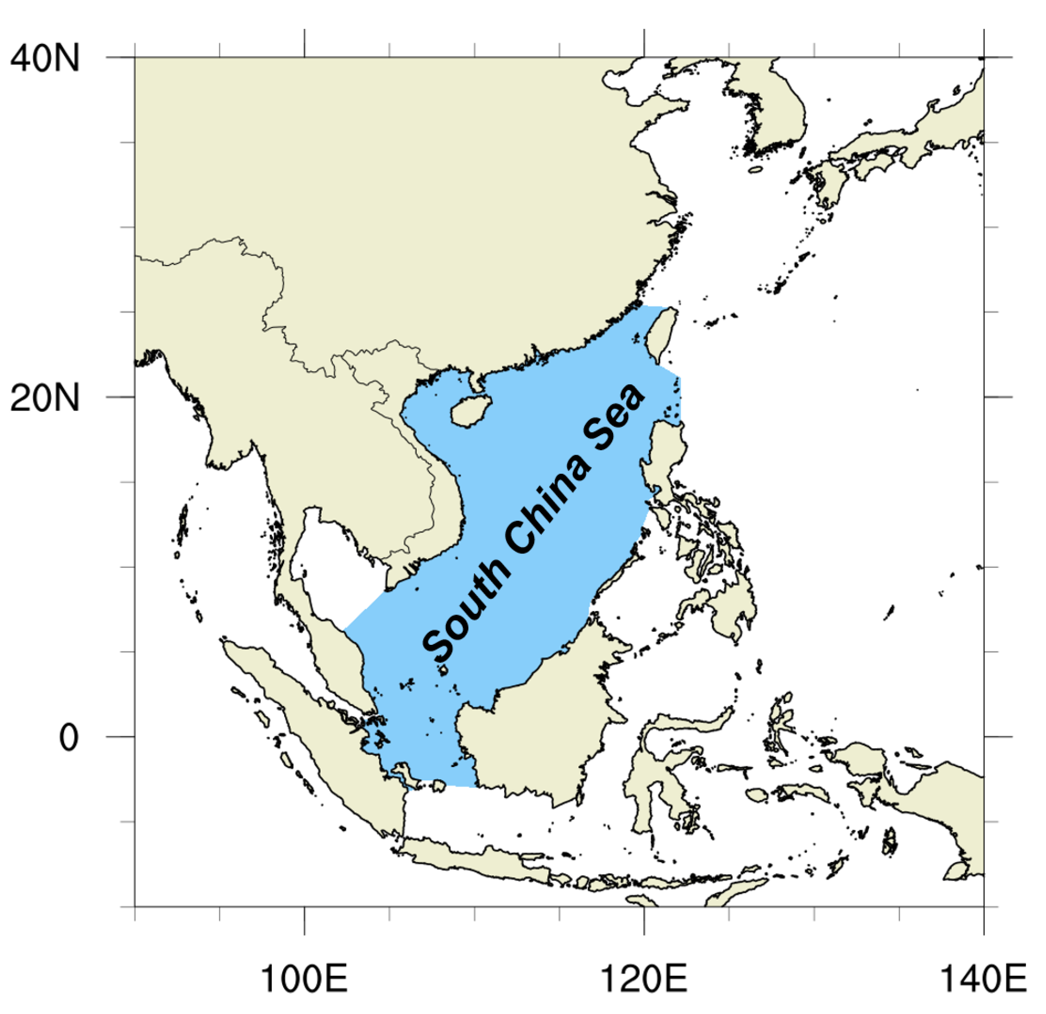
2.1. Study Area

As the largest semi-enclosed marginal sea in the northwest Pacific Ocean, SCS (Figure 1) is a hot spot for evaporation duct research. Numerous works have been published to establish a long-range radio link over South China Sea based on the evaporation duct channel [7,22,23,24]. However, without knowing the evaporation duct height, it is difficult to calculate the statistics of fading variations of the channel to estimate the fade margin to establish reliable high data rate wireless communication via evaporation duct. In this view, analysis of EDH characteristic over SCS is of particular concern for the present study.

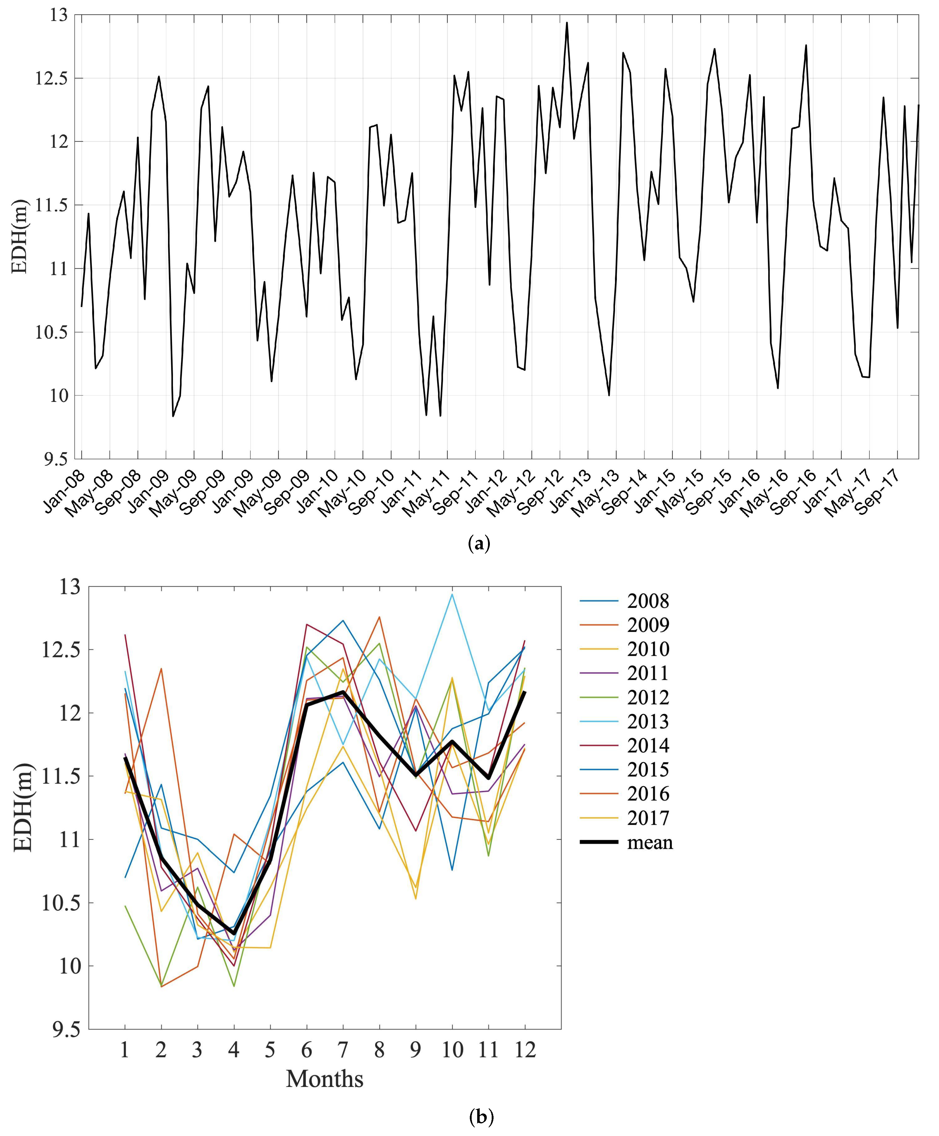
2.2. Monthly EDH Data

The monthly mean of EDH data from 2008 to 2017 has been retrieved from air-sea environmental data using evaporation duct model [25]. Based on the Monin-Obukhov similarity and Liu-Katsaros-Businger theories, the evaporation duct model estimates the EDH from local air-sea environmental conditions, including air temperature, sea surface temperature, specific humidity, surface wind speed, and pressure [26,27]. More details about the basic theory, model algorithm and parameterization schemes can be found in the authors’ recently published studies [6,7,8]. In our study, the data of air-sea variables are obtained from the reanalysis products of the National Centers for Environmental Prediction (NCEP) Climate Forecast System Reanalysis (CFSR) dataset [28]. A series of studies has been conducted on the comparison and evaluation of the EDH data obtained from this hybrid method with the measuring results from different sea areas including the South China Sea [6,20,29]. The studies have demonstrated satisfactory agreement between the retrieved EDH and practically measured EDH data, thus rendering the methodology suitable for the EDH monitoring and research. As a result, the application of stochastic time series modeling on the long-term monthly mean EDH can be performed with great accuracy.

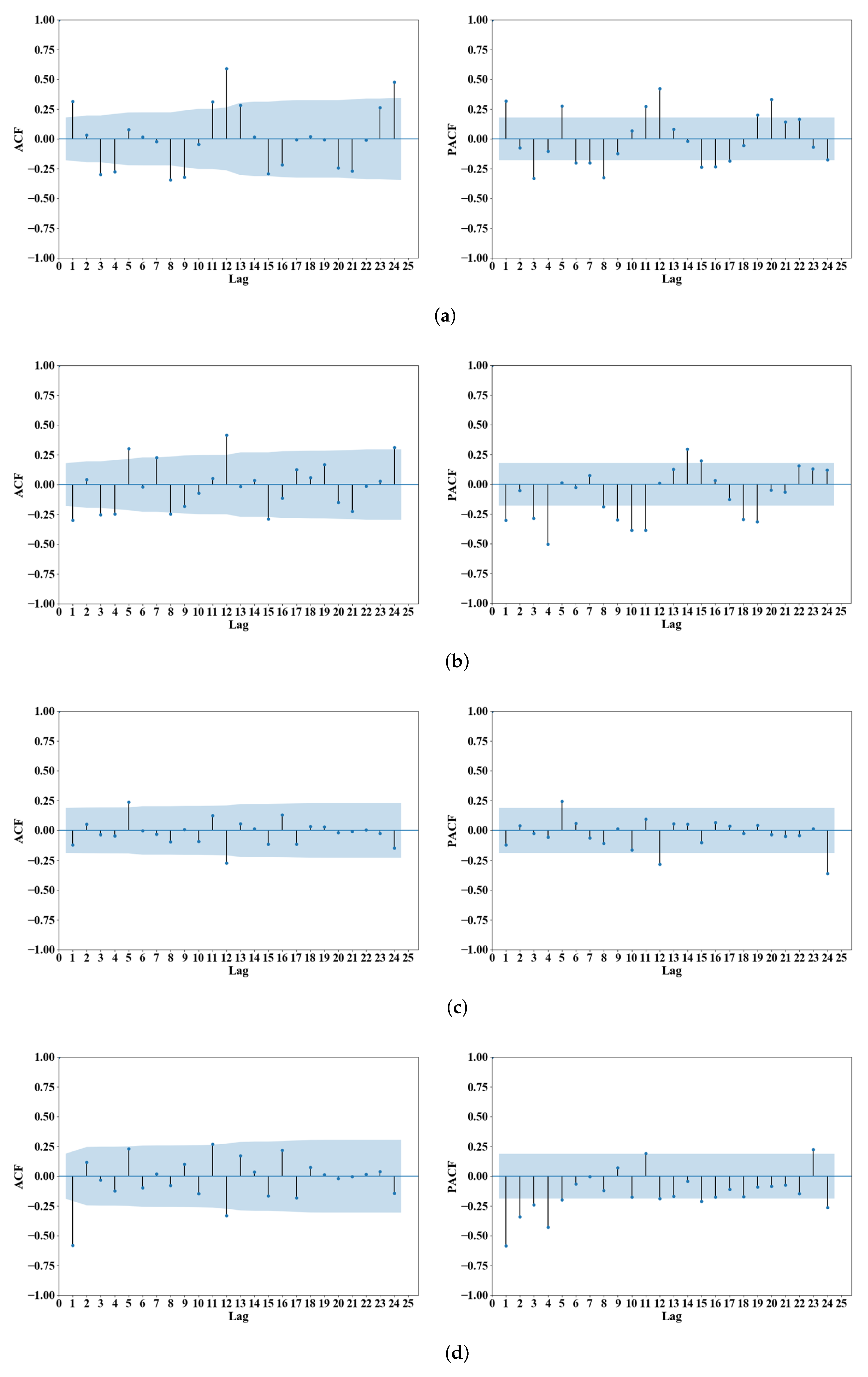
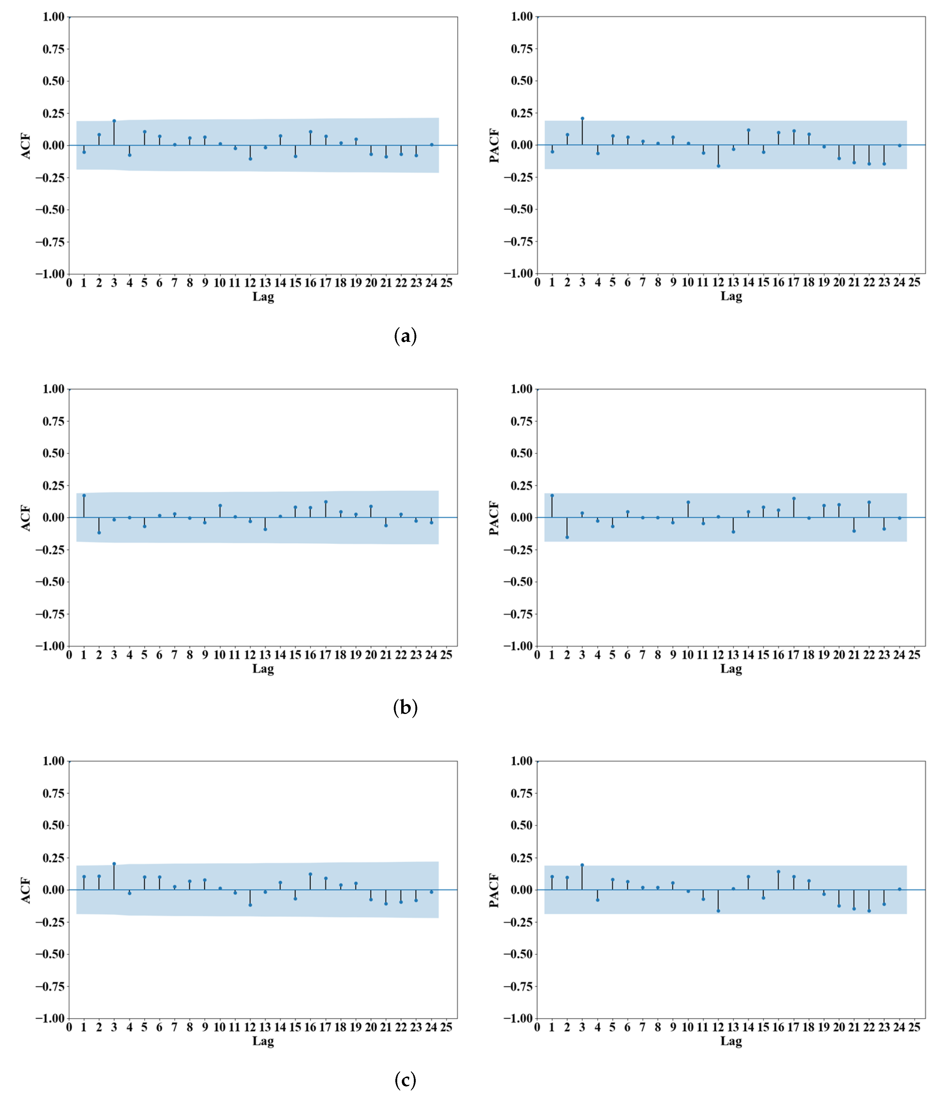
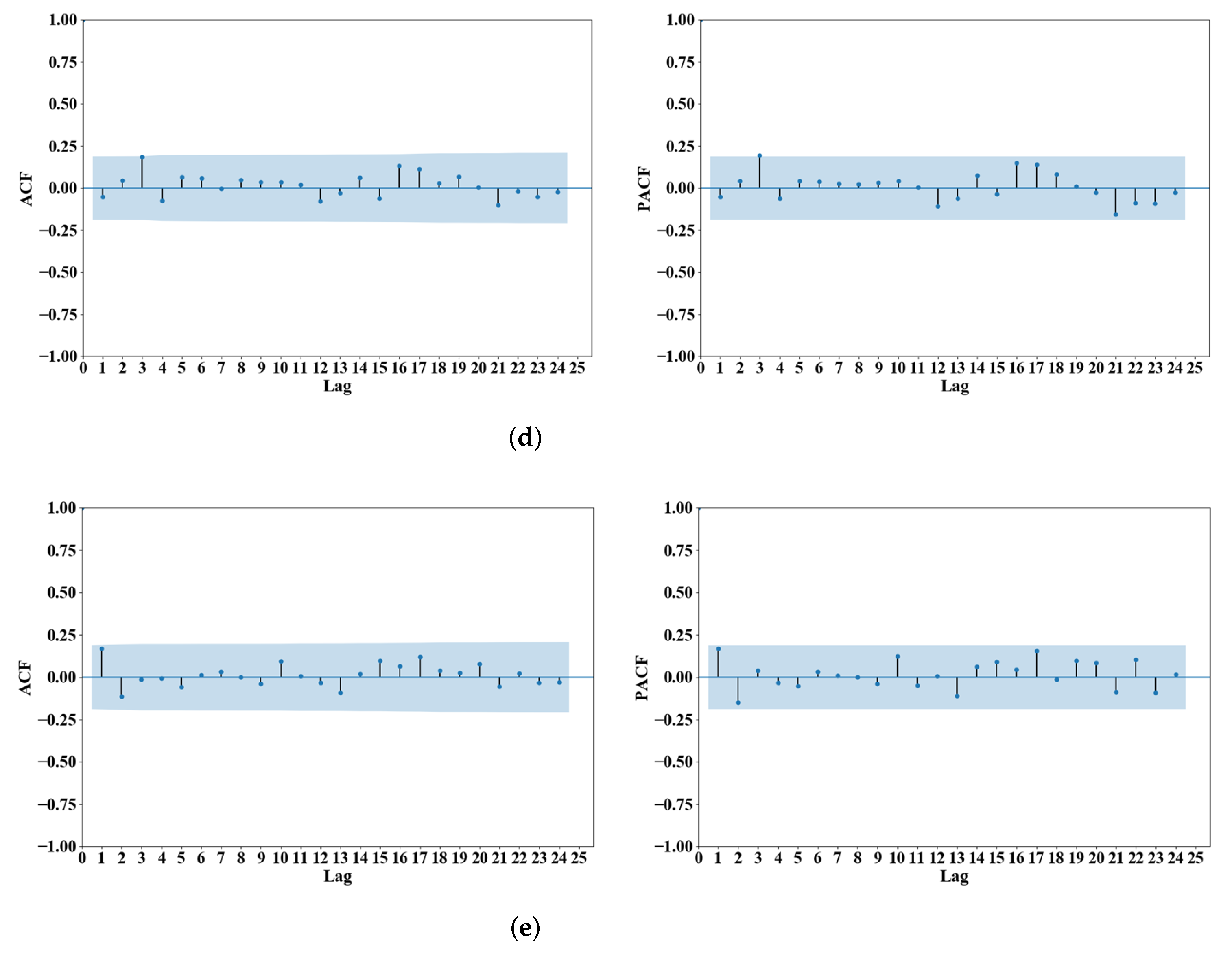
2.3. ARIMA Modeling Approach

ARIMA model consists of three parts, namely, AutoRegression, Integration and Moving Average. The autoregression part with lag order p refers to the current values $X_t$ as a function of past time series values $X_{t-1}$, $X_{t-2}$, $...$, $X_{t-p}$ and can be written as

$$\begin{array}{cc}\hfill X_t=& {\varphi }_1{X}_{t-1}+{\varphi }_2{X}_{t-2}+...+{\varphi }_p{X}_{t-p}+{\epsilon }_t\hfill \end{array}$$

(1)

where t denotes the time indices and the terms ${\varphi }_1$, ${\varphi }_2$, $...$, ${\varphi }_p$ are autoregressive coefficients that relate $X_t$ to $X_{t-1}$, $X_{t-2}$, $...$, $X_{t-p}$.

The moving average part of the model with lag q can be expressed in following form

$$\begin{array}{c}\hfill X_t={\epsilon }_t-{\theta }_1{\epsilon }_{t-1}-{\theta }_2{\epsilon }_{t-2}-...-{\theta }_q{\epsilon }_{t-q}\end{array}$$

(2)

where ${\epsilon }_{t-1}$, ${\epsilon }_{t-2}$, $...$, ${\epsilon }_{t-p}$ are the independent white noise sequence with zero mean and variance ${\sigma }^2$. ${\theta }_1$, ${\theta }_2$, $...$, ${\theta }_q$ are the moving average coefficients relating $X_t$ to ${\epsilon }_{t-1}$, ${\epsilon }_{t-2}$, $...$, ${\epsilon }_{t-p}$. If the time series is not stationary, differencing should be applied to stationalize the time series and this should correspond to the integration in the model with lag d. Hence, the ARIMA (p,d,q) can be mathematically written as

$$\varphi \left(B\right){(1-B)}^d{X}_t=\theta \left(B\right){\epsilon }_t$$

(3)

where B is the backshift operator, i.e., $B{X}_t=X_{t-1}$. The terms $\varphi \left(B\right)$ and $\theta \left(B\right)$ are the autoregressive and moving average operators, respectively, and can be written as

$$\varphi \left(B\right)=1-{\varphi }_1{B}^1-{\varphi }_2{B}^2-...-{\varphi }_p{B}^p$$

(4)

$$\theta \left(B\right)=1-{\theta }_1{B}^1-{\theta }_2{B}^2-...-{\theta }_q{B}^q$$

(5)

When the time series contains seasonality, a multiplicative seasonal ARIMA denoted as ARIMA (p,d,q) × (P,D,Q)${}_s$ is applied, where P,D,Q represent seasonal autoregression, seasonal differencing and seasonal moving average orders, respectively, and s denotes the seasonal cycle. The seasonality in the time series can be determined by the correlation function examing the lags significantly different from zero. A seasonal ARIMA (p,d,q) × (P,D,Q) built for the time series is defined as follows:

$${\varphi }_p\left(B\right){\Phi }_p\left(B^s\right){(1-B)}^d{X}_t={\theta }_q\left(B\right){\mathsf{\Theta }}_Q\left(B^s\right){\epsilon }_t$$

(6)

where B is the backshift or lag operator, s is the seasonal lag (in month for present study), ${\epsilon }_t$ represents error variables, d and D are non-seasonal and seasonal difference, $\varphi$ and $\Phi$ are the non-seasonal and seasonal autoregressive parameters, and $\theta$ and $\mathsf{\Theta }$ are the non-seasonal and seasonal moving parameters, respectively.

The methodology of ARIMA modeling approach contains iterative procedures to find the best-fit model of the internal structures of the time series through three steps, namely, identification, estimation and diagnostic checking. To identify a suitable model, the stationarity of the time series should be checked firstly. For non-stationarity time series, it is necessary to employ situable differencing process to achieve stationarity. The autoregression and moving average parts of the differenced time series are determined by the graphs of autocorrelation function (ACF) and partial autocorrelation function (PACF). Considering the ACF and PACF correlograms, several ARIMA models are identified as the alternatives. The best-fit model is mainly determined by normalized Bayesian information criterion (BIC) value. BIC is a comprehensive parameter to measure the overall fitness of a model as following equation

$$\mathrm{BIC}=-2ln\left(l_{max}\right)/n+kln\left(n\right)/n$$

(7)

where $l_{max}$ is the model’s maximum likelihood and n and k are the sample size and the number of estimated parameters, respectively.

If the preferred model is obtained, the next step is to estimate the model parameters. Once the model parameters are specified, ACF and PACF correlograms of the residuals, and the difference between the actual and fitted data, are plotted for diagnostic check. For a good ARIMA model, the residuals should be uncorrelated and distributed normally with a zero mean. At last, the best-fit model is used to forecast the future values of current time series.

2.4. Model Verification and Comparison Criteria

Several different consistency measures, including the root of the mean square error (RMSE) and mean absolute percentage error (MAPE), are adopted to evaluate the performances of proposed model. These two quantified error measures are given by

$$\mathrm{RMSE}=\sqrt{\frac{1}{N}\sum _{i=1}^N{(P_i-X_i)}^2}$$

(8)

$$\mathrm{MAPE}=\frac{1}{N}\sum _{i=1}^N\left|\frac{P_i-X_i}{P_i}\right|\times 100\%$$

(9)

where $P_i$ and $X_i$ are the predicted and observed values, respectively. N is the number of data.

3. Results and Discussion

3.1. Annual and Monthly EDH Variability

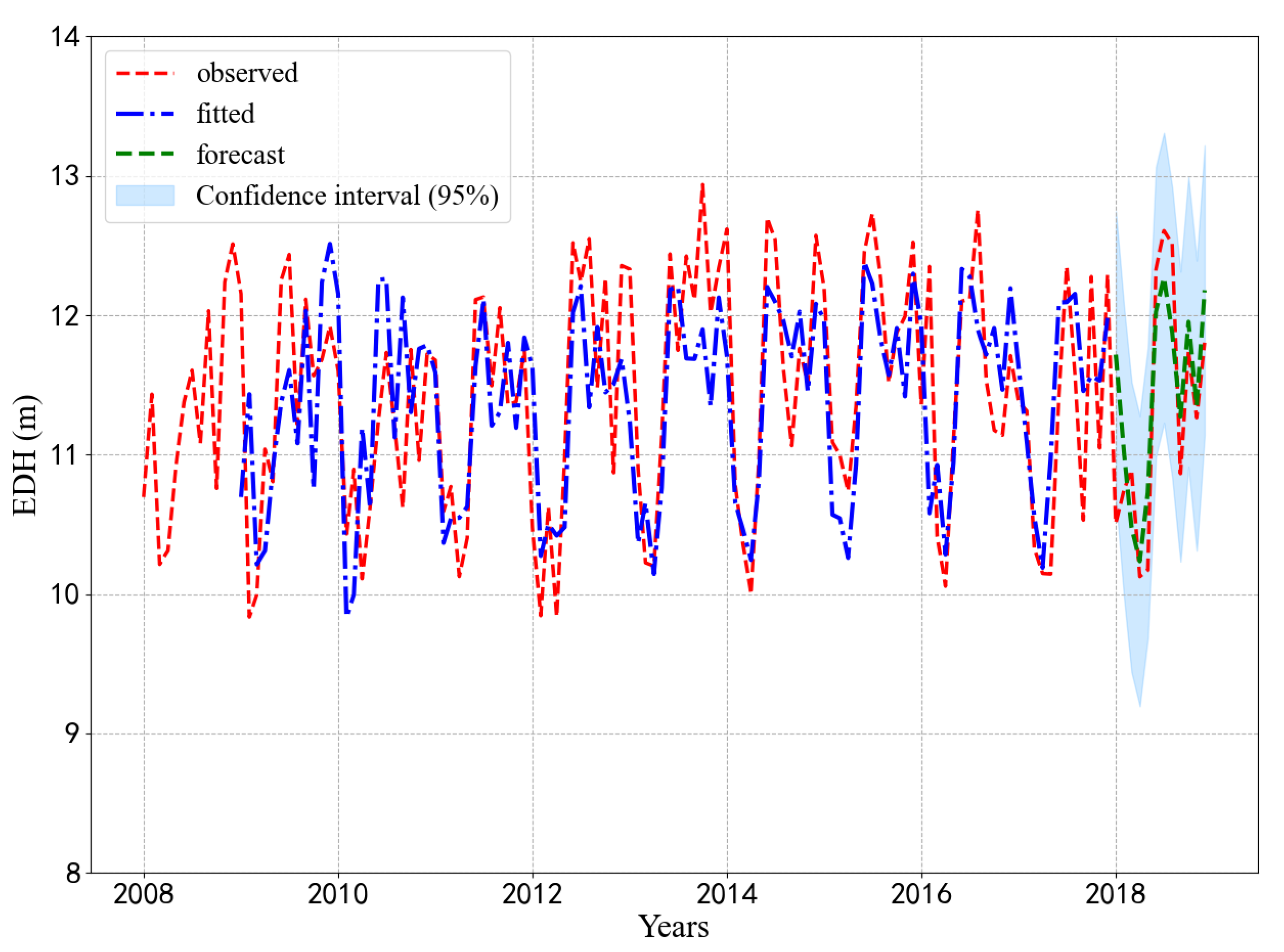
Figure 2a depicts the trend of evaporation duct height over the South China Sea from January to December in 10 years (2008–2017), where the bold black curve stands for the mean values. Figure 2b shows the long-term monthly average EDH variation over SCS from January 2008 to December 2017. There is a common trend of EDH observed in the seasons of each year. Generally, the overall level of EDH from January to May is lower than that of June to December. The peak values appear in June and July, and the nadirs are observed in the months of March and April. This variation is mainly attributed to the seasonal monsoon over the South China Sea [9]. The SCS is governed by the Southwest monsoon and northeast monsoon in summer and winter, respectively. Our previous research has pointed out that the evaporation duct height over South China Sea shows strong relevant to the sea surface wind and SST. The seasonality of the wind and SST patterns is charged for the seasonal variability in the EDH over the SCS. Further, the seasonality in the time series can be adpoted in the statistical model to determine the future trends of EDH.

3.2. ARIMA Modeling

The establishment of ARIMA model contains several iterative procedures, including model identification, model parameters estimation and model diagnostic checking. The monthly EDH data from 2008 to 2017 are used to train and obtain the optimal ARIMA model.

The model identification is mainly based on the autocorrelation function (ACF) and partial autocorrelation function (PACF) correlograms of the monthly EDH time series. Autocorrelation describes the correlations between each pair of points in the time series with a specific lag. Partial autocorrelation is used to identify the correlations between time series points with different lags. If the ACF and PACF sequence rapidly converges to zero with increasing lag values, the sequence is considered stationary. Figure 3 shows the ACF and PACF correlograms of the EDH time series with different differential options. The x-axis is the time lag indicating the separation steps, and the y-axis is the correlation value between $-1$ and +1. The blue shade represents the 95% confidence intervals.

Table 1. Estimated BIC values of different ARIMA models fitted to the data.

Model Num.	Model	BIC	RMSE	MAPE
1	(0,0,1) × (0,1,2)${}_{12}$	150.426	0.604	0.042
2	(1,0,1) × (0,1,2)${}_{12}$	150.649	1.066	0.051
3	(0,0,0) × (0,1,2)${}_{12}$	151.578	0.612	0.043
4	(1,0,0) × (0,1,2)${}_{12}$	152.178	0.605	0.043
5	(1,0,2) × (0,1,2)${}_{12}$	153.337	1.044	0.051

summarizes the BIC, RMSE and MAPE values of five best models among the different combinations of ARIMA model parameters to the data.

Figure 4 gives the ACF and PACF between the residuals at various lags of the five ARIMA models. Globally, the lags of all cases satisfy the 95% confidence criteria. Considering the autocorrelation coefficients of the residuals, all 24 autocorrelation coefficients are not statistically significant. This indicates that the residuals are similar to white noise and the models are a good fit. Individually, the model ARIMA (0,0,1) × (0,1,2)${}_{12}$ has the minimum BIC value and smallest RMSE and MAPE. As a result, model ARIMA (0,0,1) × (0,1,2)${}_{12}$ is considered as the best fit model and could be further applied in the following forecasts and analysis.

Once the model parameters are estimated, the model diagnostic checking is then performed, and a forecast of EDH for the next 12 months till December 2018 has been made at a 95% level of confidence. Figure 5 shows that the selected ARIMA model could simulate the seasonality well from the periodicity in the historical EDH series. The major feature of ARIMA model is that this modeling technique is rather simple and only fewer parameters are needed to make a good prediction. However, the random large fluctuations existing in the data that led to these extreme values may not be well represented by the model. Further evaluation of the model is conducted to compare the forecast values with the observed data till December 2018.

Table 2. Residuals of predicted and actual values of EDH for the model ARIMA (0,0,1) × (0,1,2)${}_{12}$ (unit:m).

Months	Actual	Predicted	Residuals
January 2018	10.508	11.718	−1.210
February 2018	10.747	11.017	−0.270
March 2018	10.887	10.480	0.407
April 2018	10.124	10.235	−0.111
May 2018	10.171	10.728	−0.557
June 2018	12.326	12.024	0.302
July 2018	12.607	12.268	0.339
August 2018	12.512	11.876	0.636
September 2018	10.863	11.273	−0.410
October 2018	11.748	11.954	−0.206
November 2018	11.264	11.351	−0.087
December 2018	11.803	12.180	−0.377

shows the residuals between the predicted and observed data are within ±0.5 for the whole period, except for the months of January and August. This may result from the linear characteristics of the ARIMA model [10,12]. Recently, a new software package, namely, Jumps Upon Spectrum and Trend (JUST), has been proposed to detect potential jumps in non-stationary time series and predict future trends [30,31]. This method is based on the spectral analysis and may also solve the non-stationary EDH time series forecasting. This will be part of our next research project. Generally, the prediction accuracy of the selected ARIMA (0,0,1) × (0,1,2)${}_{12}$ is satisfactory and the model can be further extended to the months where the observed data are not available.

4. Conclusions

The study discusses the stochastic modeling of evaporation duct height over South China Sea for the period from 2008 to 2017. ARIMA models are analyzed to fit and forecast the monthly EDH data. Seasonal differencing is used to remove the seasonality and make the time series stationary. Correlation analysis is conducted to the differenced series in terms of the ACF and PACF, and the significant lags are adopted to calculate the order of the ARIMA models. Based on evaluation criteria, it is found that ARIMA (0,0,1) × (0,1,2)${}_{12}$ model is adequate for simulating the EDH. Further, prediction has been conducted based on the proposed model for the year 2018. The results shows a high degree of fitness between the forecasted and observed values. Obviously, there are also some discrepancies, which probably come from the inherent linearity of the model. Improving the forecasting ability of our proposed model should be part of our future work.

References

1. Dinc, E.; Akan, O. Beyond-line-of-sight communications with ducting layer. IEEE Commun. Mag. 2014, 10, 37–43. [Google Scholar] [CrossRef]
2. Wang, J.; Zhou, H.; Li, Y.; Sun, Q.; Wu, Y.; Jin, S.; Quek, T.Q.; Xu, C. Wireless channel models for maritime communications. IEEE Access 2018, 6, 68070–68088. [Google Scholar] [CrossRef]
3. Woods, G.S. High-Capacity, Long-Range, Over ocean microwave link using the evaporation duct. IEEE J. Ocean. Eng. 2009, 3, 323–330. [Google Scholar] [CrossRef]
4. Zhang, Q.; Yang, K.D.; Shi, Y.; Yan, X.D. Oceanic propagation measurement in the northern part of the South China Sea. In Proceedings of the IEEE OCEANS 2016-Shanghai, Shanghai, China, 10–13 April 2016. [Google Scholar]
5. Zhang, Q.; Yang, K.D. Study on evaporation duct estimation from point-to-point propagation measurements. IET Sci. Meas. Technol. 2018, 4, 456–460. [Google Scholar] [CrossRef]
6. Shi, Y.; Yang, K.D.; Yang, Y.X.; Ma, Y.L. A new evaporation duct climatology over the South China Sea. J. Meteorol. Res. 2015, 5, 764–778. [Google Scholar] [CrossRef]
7. Zhang, Q.; Yang, K.D.; Shi, Y. Spatial and temporal variability of the evaporation duct in the Gulf of Aden. Tellus A 2016, 68, 29792. [Google Scholar] [CrossRef] [Green Version]
8. Yang, K.D.; Zhang, Q.; Shi, Y.; He, Z.Y.; Lei, B.; Han, Y.N. On Analyzing Space-time Distribution of Evaporation Duct Height over the Global Ocean. Acta Oceanol. Sin. 2016, 7, 20–29. [Google Scholar] [CrossRef]
9. Yang, K.D.; Zhang, Q.; Shi, Y. Interannual variability of the evaporation duct over the South China Sea and its relations with regional evaporation. J. Geophys. Res. Oceans 2017, 8, 6698–6713. [Google Scholar] [CrossRef]
10. Ghaderpour, E.; Pagiatakis, S.D.; Hassan, Q.K. A Survey on Change Detection and Time Series Analysis with Applications. Appl. Sci. 2021, 11, 6141. [Google Scholar] [CrossRef]
11. Box, G.E.P.; Jenkins, G.M.; Reinsel, G.C.; Ljung, G.M. Time Series Analysis: Forecasting and Control; John Wiley and Sons Inc.: Hoboken, NJ, USA, 2015; p. 712. [Google Scholar]
12. Kozitsin, V.; Katser, I.; Lakontsev, D. Online Forecasting and Anomaly Detection Based on the ARIMA Model. Appl. Sci. 2021, 11, 3194. [Google Scholar] [CrossRef]
13. Sim, S.K.; Maass, P.; Lind, P.G. Wind speed modeling by nested ARIMA processes. Energies 2019, 12, 69. [Google Scholar] [CrossRef] [Green Version]
14. Eymen, A.; Köylü, Ü. Seasonal trend analysis and ARIMA modeling of relative humidity and wind speed time series around Yamula Dam. Meteorol. Atmos. Phys. 2019, 3, 601–612. [Google Scholar] [CrossRef]
15. Odai, A.; Babbar, R.; Karmaker, T. Trend analysis and ARIMA modeling for forecasting precipitation pattern in Wadi Shueib catchment area in Jordan. Arab. J. Geosci. 2019, 2, 27. [Google Scholar]
16. Wang, H.; Huang, J.J.; Zhou, H.; Zhao, L.X.; Yuan, Y.B. An Integrated Variational Mode Decomposition and ARIMA Model to Forecast Air Temperature. Sustainability 2019, 11, 4018. [Google Scholar] [CrossRef] [Green Version]
17. Salles, R.; Mattos, P.; Iorgulescu, A.D.; Bezerra, E.; Lima, L.; Ogasawara, E. Evaluating temporal aggregation for predicting the sea surface temperature of the Atlantic Ocean. Ecol. Inform. 2016, 36, 94–105. [Google Scholar] [CrossRef]
18. Natsagdorj, E.; Renchin, T.; Maeyer, P.D.; Darkhijav, B. Spatial Distribution of Soil Moisture in Mongolia Using SMAP and MODIS Satellite Data: A Time Series Model (2010–2025). Remote Sens. 2021, 13, 347. [Google Scholar] [CrossRef]
19. Yang, S.B.; Liu, S.H.; Li, X.F.; Zhong, Y.; He, X.; Wu, C. The short-term forecasting of evaporation duct height (EDH) based on ARIMA model. Multimed. Tools Appl. 2016, 23, 24903–24916. [Google Scholar] [CrossRef]
20. McKeon, B.D. Climate Analysis of Evaporation Ducts in the South China Sea. Master’s Thesis, Naval Postgraduate School, Monterey, CA, USA, 2013. [Google Scholar]
21. Zaidi, K.S.; Jeoti, V.; Drieberg, M.; Awang, A.; Iqbal, A. Fading characteristics in evaporation duct: Fade margin for a wireless link in the South China Sea. IEEE Access 2018, 6, 11038–11045. [Google Scholar] [CrossRef]
22. Shi, Y.; Yang, K.D.; Yang, Y.X.; Ma, Y.L. Experimental verification of effect of horizontal inhomogeneity of evaporation duct on electromagnetic wave propagation. Chin. Phys. B 2015, 4, 044102. [Google Scholar] [CrossRef]
23. Shi, Y.; Yang, K.D.; Yang, Y.X.; Ma, Y.L. Influence of obstacle on electromagnetic wave propagation in evaporation duct with experiment verification. Chin. Phys. B 2015, 4, 054101. [Google Scholar] [CrossRef]
24. Shi, Y.; Zhang, Q.; Wang, S.W.; Yang, K.D.; Yang, Y.X.; Yan, X.D.; Ma, Y.L. A comprehensive study on maximum wavelength of electromagnetic propagation in different evaporation ducts. IEEE Access 2019, 7, 82308–82319. [Google Scholar] [CrossRef]
25. Zhang, Q.; Yang, K.D.; Yang, Q.L. Statistical analysis of the quantified relationship between evaporation duct and oceanic evaporation for unstable conditions. J. Atmos. Ocean. Technol. 2017, 11, 2489–2497. [Google Scholar] [CrossRef]
26. Babin, S.M.; Dockery, G.D. LKB-based evaporation duct model comparison with buoy data. J. Appl. Meteorol. 2002, 4, 434–446. [Google Scholar] [CrossRef]
27. Frederickson, P.A.; Davidson, K.L.; Goroch, A.K. Operational Bulk Evaporation Duct Model for MORIAH Version 1.2.; Tech. Rep.; Naval Postgraduate School: Monterey, CA, USA, 2000. [Google Scholar]
28. Saha, S.; Moorthi, S.; Pan, H.L.; Wu, X.; Wang, J.; Nadiga, S.; Tripp, P.; Kistler, R.; Woollen, J.; Behringer, D.; et al. The NCEP climate forecast system reanalysis. Bull. Am. Meteorol. Soc. 2010, 8, 1015–1058. [Google Scholar] [CrossRef]
29. Frederickson, P.A.; Murphree, J.T.; Twigg, K.L.; Barrios, A. A modern global evaporation duct climatology. In Proceedings of the IEEE International Conference on Radar, Adelaide, SA, Australia, 2–5 September 2008; pp. 292–296. [Google Scholar]
30. Ghaderpour, E.; Vujadinovic, T. Change Detection within Remotely Sensed Satellite Image Time Series via Spectral Analysis. Remote Sens. 2020, 12, 4001. [Google Scholar] [CrossRef]
31. Ghaderpour, E.; Vujadinovic, T. The Potential of the Least-Squares Spectral and Cross-Wavelet Analyses for Near-Real-Time Disturbance Detection within Unequally Spaced Satellite Image Time Series. Remote Sens. 2020, 12, 2446. [Google Scholar] [CrossRef]
Figure 1. Location of the study area: South China Sea (shaded in blue).
Atmosphere 12 01663 g001
Figure 2. Monthly Variation of EDH during 2008–2017 over South China Sea (a) monthly trend (b) long-term monthly average.
Atmosphere 12 01663 g002
Figure 3. ACF and PACF plots of EDH time series with different differencing combinations: (a) ithout differencing, (b) with non-seasonal differencing, (c) with seasonal differencing and (d) with non-seasonal and seasonal differencing both.
Atmosphere 12 01663 g003
Figure 4. Estimated residual ACF and PACF using different ARIMA models. (a) ARIMA (0,0,1) × (0,1,2) 12 . (b) ARIMA (1,0,1) × (0,1,2) 12 . (c) ARIMA (0,0,0) × (0,1,2) 12 . (d) ARIMA (1,0,0) × (0,1,2) 12 . (e) ARIMA (1,0,2) × (0,1,2) 12 .
Atmosphere 12 01663 g004aAtmosphere 12 01663 g004b
Figure 5. Time series plots showing the observed data EDH (red line) and modeled output (blue line) values for the model ARIMA (0,0,1) × (0,1,2) 12 . The forecast values for the year 2018 (green line) are shown with the 95% confidence intervals(shaded region).
Atmosphere 12 01663 g005