Construction of a Simple Domeless Net Radiometer for Demonstrating Energy Balance Concepts in a Laboratory Activity

Abstract

Even though energy balance concepts are fundamental to solutions of problems in a number of disciplines in the agricultural and life sciences, they are seldom demonstrated in a laboratory activity. Here, we introduce a simple domeless net radiometer to demonstrate how the surface temperature of an object aboveground is regulated by the properties of the surfaces and environmental conditions. The device is based on the early designs of all-wave net radiometers and is composed of a foam disc with its opposing surfaces coated with either white or black paint. Temperatures of the disc’s surfaces are monitored using thermocouple temperature sensors. Using a combination of solar irradiance, albedo of the ground surface, air temperature, and wind speed measurements, the temperatures of the disc’s surfaces can be calculated by means of an energy balance model. We found good agreement between calculated and measured temperatures. In addition to demonstrate important physical concepts under natural outdoor conditions, we believe that the proposed laboratory activity will benefit students by allowing them to gain some experience and practical skills in working with environmental sensors, programming data acquisition systems, and analyzing data. Stimulating students’ creativity as well as developing their analytical and problem-solving skills is another goal of the proposed activity.

1. Introduction

The energy balance concept is fundamental to a number of disciplines that study how organisms and objects are influenced by the environment in which they reside (e.g., agronomy, soil science, micrometeorology, plant physiology, ecology, and hydrology). Such interactions are described by energy and mass fluxes, where the status of environmental variables and the properties of the surface of interest determine the rate of these exchanges. For example, the temperature of any surface (e.g., soil, plant, or animal) depends, in part, on how much radiation is absorbed and re-emitted, how much water is available for evaporative cooling, and how much energy is transported to or from the surface by convective currents or by thermal conduction. Because temperature is a fundamental driver of nearly all biological processes, the energy balance is intrinsically related to the growth of living organisms. Therefore, the energy balance is a unifying concept that allows one to understand how energy is absorbed and partitioned by a given surface. Undergraduate and graduate courses dealing with aspects of environmental physics usually demonstrate these concepts with numerical examples taken from textbooks [1,2] rather than in a field activity. Here, we describe an inexpensive domeless net radiometer that can be easily constructed for a laboratory activity to demonstrate how environmental conditions and surface properties determine surface temperature by means of an energy balance analysis. The device consists of a foam disc where its upper and lower surfaces are painted either black or white and its surface temperatures are monitored using thermocouple temperature sensors. The design of the disc is based on the early designs of all-wave net radiometers [3,4,5,6,7,8,9,10,11,12,13]. The goal of the activity is to demonstrate that the temperatures calculated by means of the energy balance approach follows closely those measured. We first discuss the theory necessary to obtain the solution for the disc’s energy balance, then describe its construction and how we intended its use in a laboratory experiment for an environmental physics class. Lastly, we present some data from a laboratory activity using the discs that students constructed in our classes. In our discussion, we also included questions that can be posed to students in order to stimulate discussions. For example, the foam disc we used was dry, so evaporative cooling was not a component of the energy balance (an analog for a non-transpiring leaf). What would you predict to happen if the surfaces were wet? This leaves a challenge for students wanting extra credit by creating a disc with wet surfaces.

2. Materials and Methods

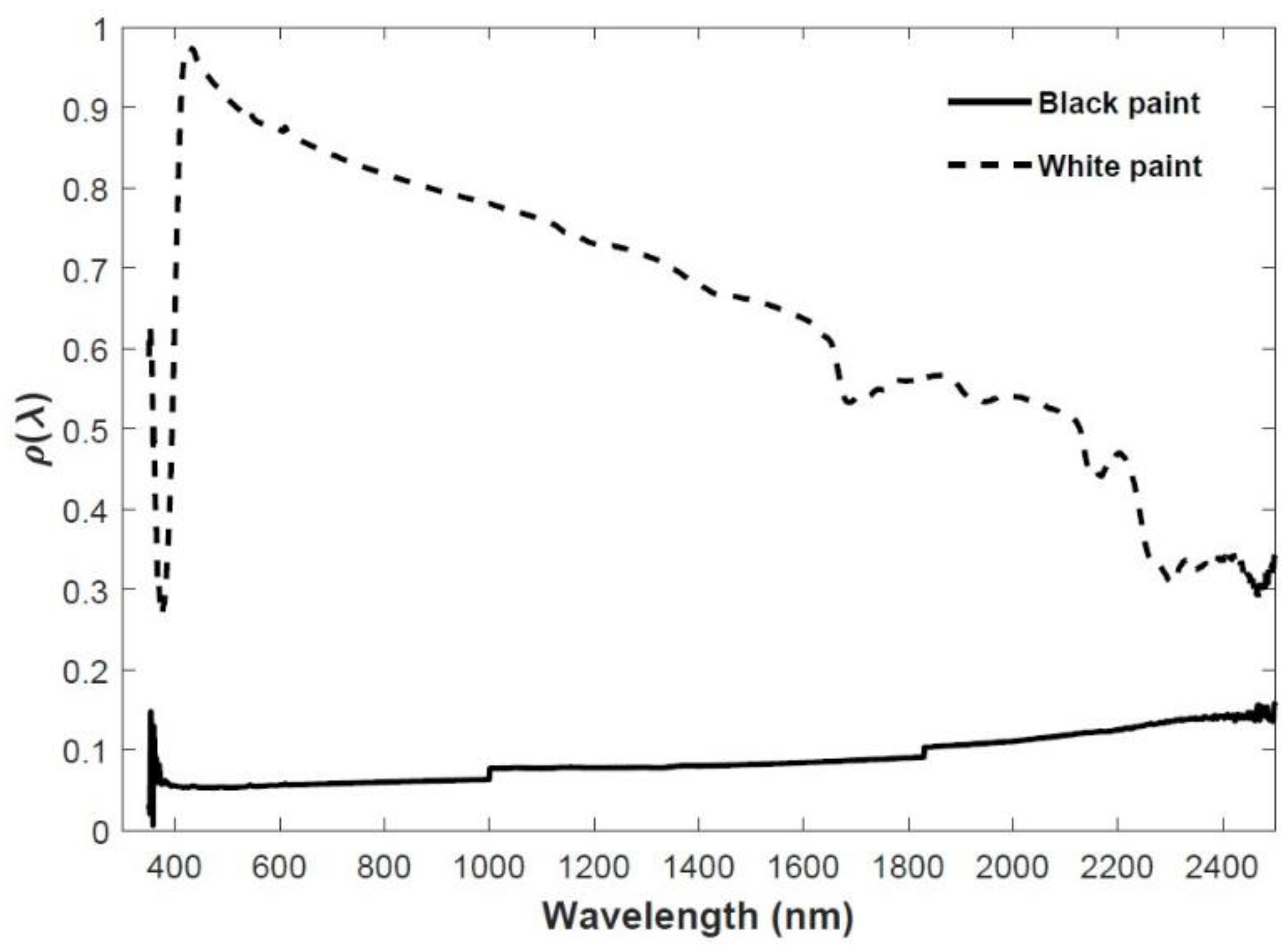
2.1. Theory

The energy balance of a surface of the disc can be written as

R_n + LE + H + G = 0,

(1)

where Rn is the net radiation, LE is the latent heat flux density (i.e., energy flux associated with evaporation of water), H is the sensible heat flux density (i.e., energy flux associated with convective air currents), and G is the energy flux density associated with conduction in the foam (heat storage ignored), all in units of W m⁻². Because the disc we used was dry, Equation (1) reduces to

R_n + H + G = 0.

(2)

If the disc is placed horizontally above the ground, Equation (2) yields

$$\left(1-{\mathsf{\rho }}_{\mathrm{U}}\right){\mathrm{R}}_{\mathrm{s}}+{\mathsf{\epsilon }}_{\mathrm{U}}{\mathrm{LW}}_{\mathrm{i}}-{\mathsf{\epsilon }}_{\mathrm{U}}{\mathsf{\sigma }\mathrm{T}}_{\mathrm{U}}^4-{\mathrm{g}}_{\mathrm{Ha}}{\mathrm{c}}_{\mathrm{p}}\left({\mathrm{T}}_{\mathrm{U}}-{\mathrm{T}}_{\mathrm{air}}\right)-\mathsf{\lambda }\frac{\left({\mathrm{T}}_{\mathrm{U}}-{\mathrm{T}}_{\mathrm{L}}\right)}{\Delta \mathrm{z}}=0$$

(3)

where ρ_U is the albedo of the upper surface of the disc, R_s is solar irradiance, ε_U is the thermal emissivity of the upper surface, LW_i is the incoming longwave radiation from the sky, σ is the Stefan–Boltzmann constant (5.67 × 10⁻⁸ W m⁻² K⁻⁴), T_U is the temperature of the upper surface (K), g_Ha is the convective conductance for heat transport (mol m⁻² s⁻¹), c_p is the specific heat of air (29.3 J mol⁻¹ K⁻¹), T_air is the air temperature (K), λ is the thermal conductivity of the foam from which the disc was constructed (W m⁻¹ K⁻¹), T_L is the temperature of the lower surface of the disc (K), and Δz is the thickness of the disc (m). Similarly, the energy balance equation for the lower surface of the disc can be written as

$$\left(1-{\mathsf{\rho }}_{\mathrm{L}}\right){\mathrm{R}}_{\mathrm{sr}}+{\mathsf{\epsilon }}_{\mathrm{L}}{\mathrm{LW}}_{\mathrm{e}}-{\mathsf{\epsilon }}_{\mathrm{L}}{\mathsf{\sigma }\mathrm{T}}_{\mathrm{L}}^4-{\mathrm{g}}_{\mathrm{Ha}}{\mathrm{c}}_{\mathrm{p}}\left({\mathrm{T}}_{\mathrm{L}}-{\mathrm{T}}_{\mathrm{air}}\right)-\mathsf{\lambda }\frac{\left({\mathrm{T}}_{\mathrm{L}}-{\mathrm{T}}_{\mathrm{U}}\right)}{\Delta \mathrm{z}}=0$$

(4)

where ρ_L is albedo of the lower surface, R_sr is the reflected solar irradiance from the ground surface beneath the disc, ε_L is the thermal emissivity of the lower surface, and LW_e is the emitted longwave radiation by the ground surface underneath the disc. The conductance g_Ha for a flat plate under laminar forced convection conditions can be calculated as [1]

$${\mathrm{g}}_{\mathrm{Ha}}=0.135\sqrt{\frac{\mathrm{u}}{\mathrm{d}}}$$

(5)

where 0.135 is constant associated with the Nusselt number (where the molar density, kinematic viscosity, and thermal diffusivity of air are evaluated at 20 °C), u is wind speed (m s⁻¹) and d is the disc characteristic dimension (m). For a circular disc, d can be calculated as [1]

$$\mathrm{d}=0.81\mathrm{w}$$

(6)

where w is the disc diameter (m). Equation (5) is multiplied by an enhancement factor to account for increased conductance under turbulent conditions (e.g., a factor of 1.25 is typically used [1]).

Values of T_U and T_L can be obtained by iterative solution of Equations (3) and (4). This can be accomplished in several ways. Microsoft Excel has an Add-In named Solver. To use Solver, two cells containing value of T_U and T_L are established. Initially, both surface temperatures are set to T_air. Two cells containing Equations (3) and (4) are then established. The sum of the absolute values of Equations (3) and (4) is calculated in a cell that is set as the objective cell whose value is to be minimized. Solver then finds values of T_U and T_L that yields the best energy balance for the combined surfaces. This Solver routine can be automated by creating a macro and can also be extended to solve many rows of data. Another possibility is to enable the iterative calculation feature on Excel to solve Equations (3) and (4). Other root finding methods can be used to find T_U and T_L, however we decided to use Solver since most students are familiar with analyzing data in Microsoft Excel.

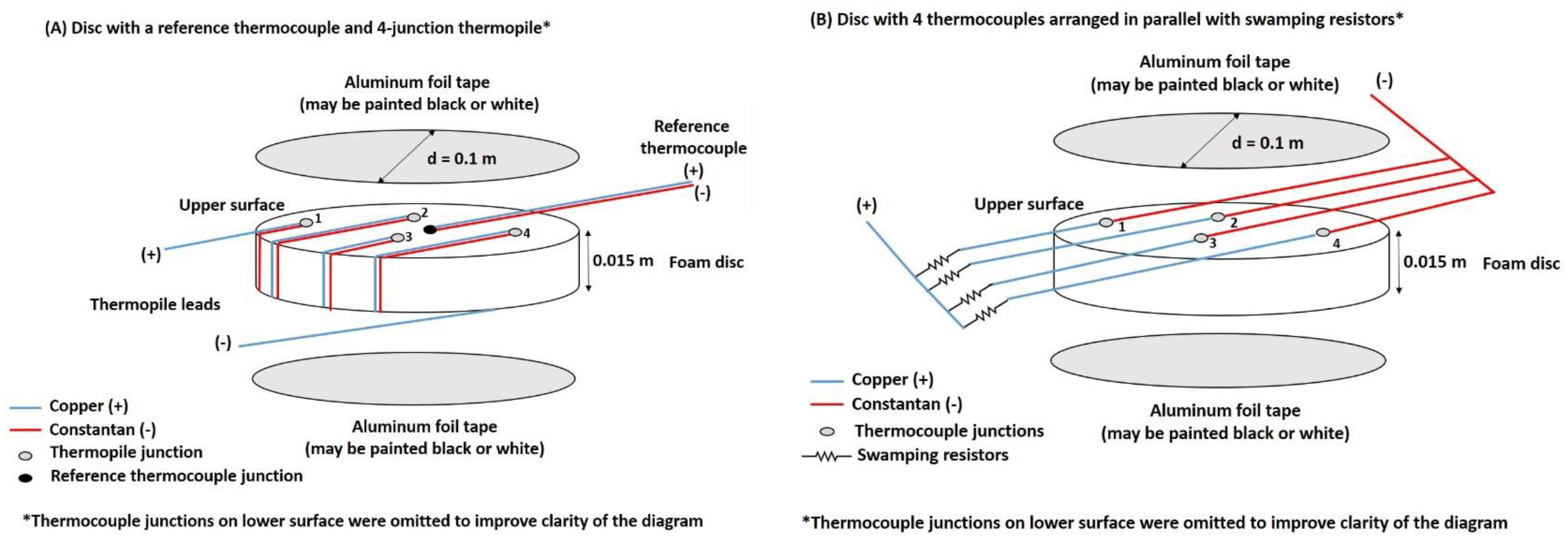
2.2. Disc Construction

The discs we built with students were made from 15 mm thick polystyrene foam cut to a diameter of 0.1 m. According to the specifications provided by the manufacturer, the foam had a thermal conductivity of 0.029 W m⁻¹ K⁻¹. Type T thermocouples were used to measure the temperature of the upper and lower surfaces [14,15,16,17,18,19,20,21,22,23,24,25,26]. Different thermocouple arrangements can be used to determine the temperature of the surfaces (Figure 1). One possibility is to place an independent thermocouple on one surface and construct a thermopile, where a number of junctions are placed on both surfaces in a series fashion, to obtain a temperature difference between the surfaces (Figure 1A). Another option is to use thermocouples connected in parallel to obtain a spatial average temperature. In such arrangement swamping resistors should be used (Figure 1B). It is generally recommended to use 200 Ω ± 1% resistors when connecting thermocouples in parallel [14]. Aluminum foil tape was used to cover both surfaces of the disc, as well as hold the thermocouple junctions in place. A small piece of cellulose acetate office tape was used to electrically isolate the thermocouple junctions before adding the aluminum foil tape. Lastly, one surface was painted black, and one was painted white with outdoor acrylic house paint. Our measurements of the spectral reflectivities in the solar radiation band (350 to 2500 nm) of the black and white paints we used are shown in Figure 2. Their albedos were determined using reference spectral solar irradiance data for an absolute air mass of 1.5 (G-173, American Society of Testing and Materials) and the following equations

$${\mathsf{\rho }}_{\mathrm{white}}=\frac{{{\displaystyle \int }}_{350}^{2500}\mathsf{\rho }\left(\mathsf{\lambda }\right)\mathrm{I}\left(\mathsf{\lambda }\right)\mathrm{d}\mathsf{\lambda }}{{{\displaystyle \int }}_{350}^{2500}\mathrm{I}\left(\mathsf{\lambda }\right)\mathrm{d}\mathsf{\lambda }}=0.80$$

(7)

$${\mathsf{\rho }}_{\mathrm{black}}=\frac{{{\displaystyle \int }}_{350}^{2500}\mathsf{\rho }\left(\mathsf{\lambda }\right)\mathrm{I}\left(\mathsf{\lambda }\right)\mathrm{d}\mathsf{\lambda }}{{{\displaystyle \int }}_{350}^{2500}\mathrm{I}\left(\mathsf{\lambda }\right)\mathrm{d}\mathsf{\lambda }}=0.06$$

(8)

where ρ(λ) is the reflectivity of the paint and I(λ) is solar irradiance at a specific wavelength (λ). The integrals were carried out numerically by means of the trapezoidal method of integration. The thermal emissivities of both paints was assumed to be 0.95. Discs built by students are shown in Figure 3.

2.3. Proposed Laboratory Activity

The objective of the laboratory activity was to compare the calculated surface temperatures of the disc surfaces to those measured using the thermocouples. The data we present in this paper are for two discs that were constructed by students and that were mounted in a mast at a height of about 0.5 m and parallel to a turf grass field. Disc 1 had the white surface facing the sky and the black surface facing the ground, whereas Disc 2 was the opposite (Figure 3b). At the same height of the discs, we also set up a four-channel net radiometer (model CNR1, Kipp & Zonen, Delft, The Netherlands), a cup anemometer (model 12102, R.M. Young Co., Traverse City, MI, USA), and a unshielded fine-wire type T thermocouple. Measurements of R_s, R_sr, LW_i, and LW_e were obtained from the net radiometer. The thermocouple provided measurements of T_air. The cup anemometer provided wind speed measurements needed to calculate g_Ha. A data logger (model CR23X, Campbell Scientific, Logan, UT, USA), controlled the sensors and measurements were averaged over 10 min intervals. The discussion of the data would be carried out during class sections as a group. Data analysis would be performed individually by the students as part of their homework.

When a net radiometer is not available, the radiation balance can be estimated using a pyranometer and an infrared thermometer (IRT). The pyranometer would provide values of R_s and R_sr can be calculated using an estimate of the albedo of the surface underneath the discs (e.g., if the surface is grass then assuming an albedo of 0.23 is adequate). Using air temperature data, LW_i can be estimated using the Stefan–Boltzmann equation and an estimate of sky emissivity (ε_sky) as [1,2]

$${\mathsf{\epsilon }}_{\mathrm{sky}}=\left(1-0.84\mathrm{c}\right)[9.2\times {10}^{-6}{\left(273.15+{\mathrm{T}}_{\mathrm{air}}\right)}^2]+0.84\mathrm{c}$$

(9)

where c is the sky cloud cover fraction. When under clear sky conditions c is set to 0, whereas under completely overcast conditions c is set to 1. The IRT may be pointed to the surface underneath the disc to obtain an estimate of surface temperature, which may then be used to estimate LW_e by means of the Stefan–Boltzmann equation. This approach to calculate the components of the radiation balance is only an approximation, and it may introduce errors in the energy balance calculations for the disc. If a four-channel net radiometer is available, its use is preferred. Lastly, students who are interested in the heat balance at night may use a 2-D sonic anemometer instead of a cup anemometer. Free convection may play an important role in sensible heat transfer in calm nights with low wind speeds. Cup anemometers are known to have stalling speeds of about 0.2 m s⁻¹ which is inappropriate for measuring low wind speeds. Equations for g_Ha under free convection conditions are given in environmental physics textbooks [1,2].

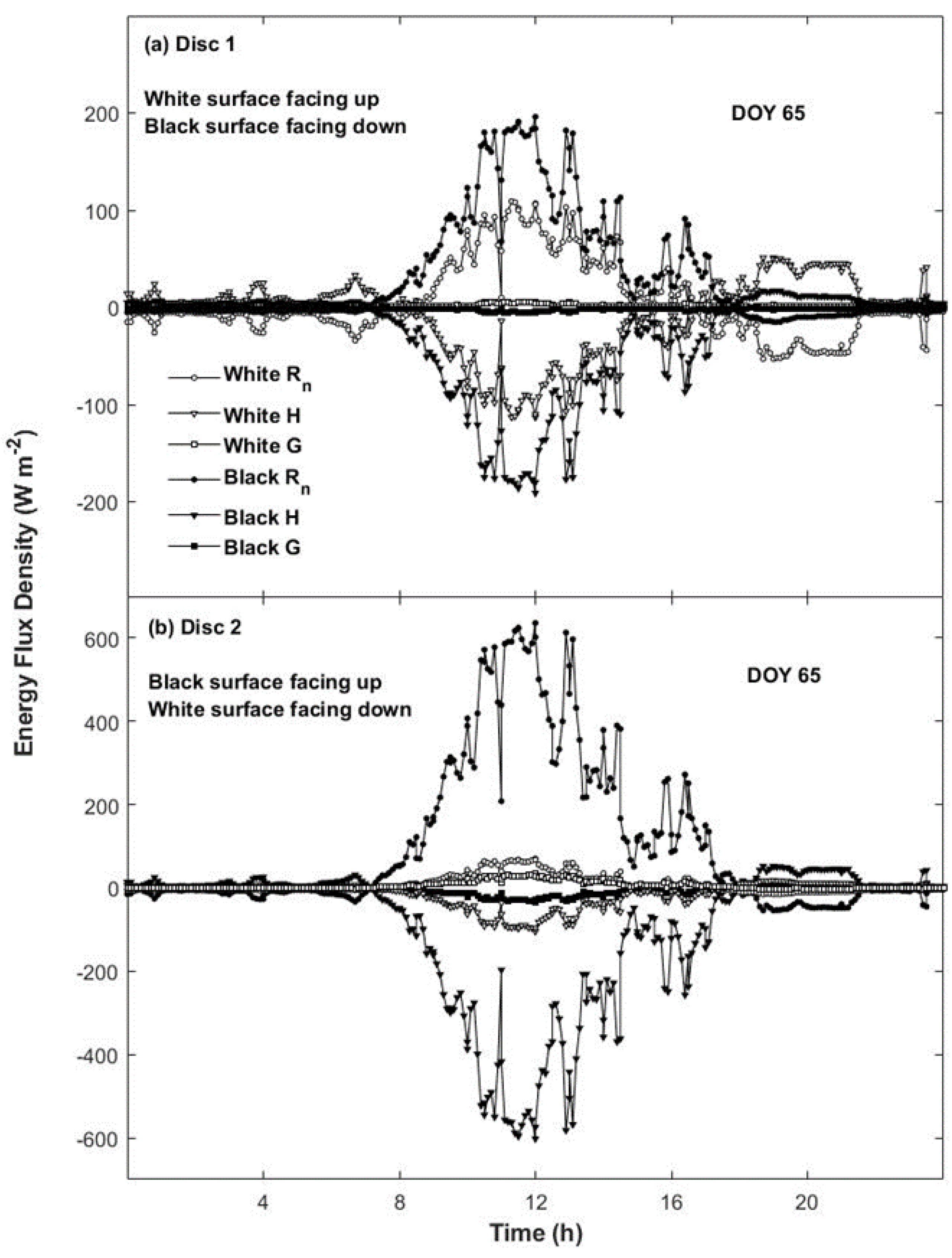
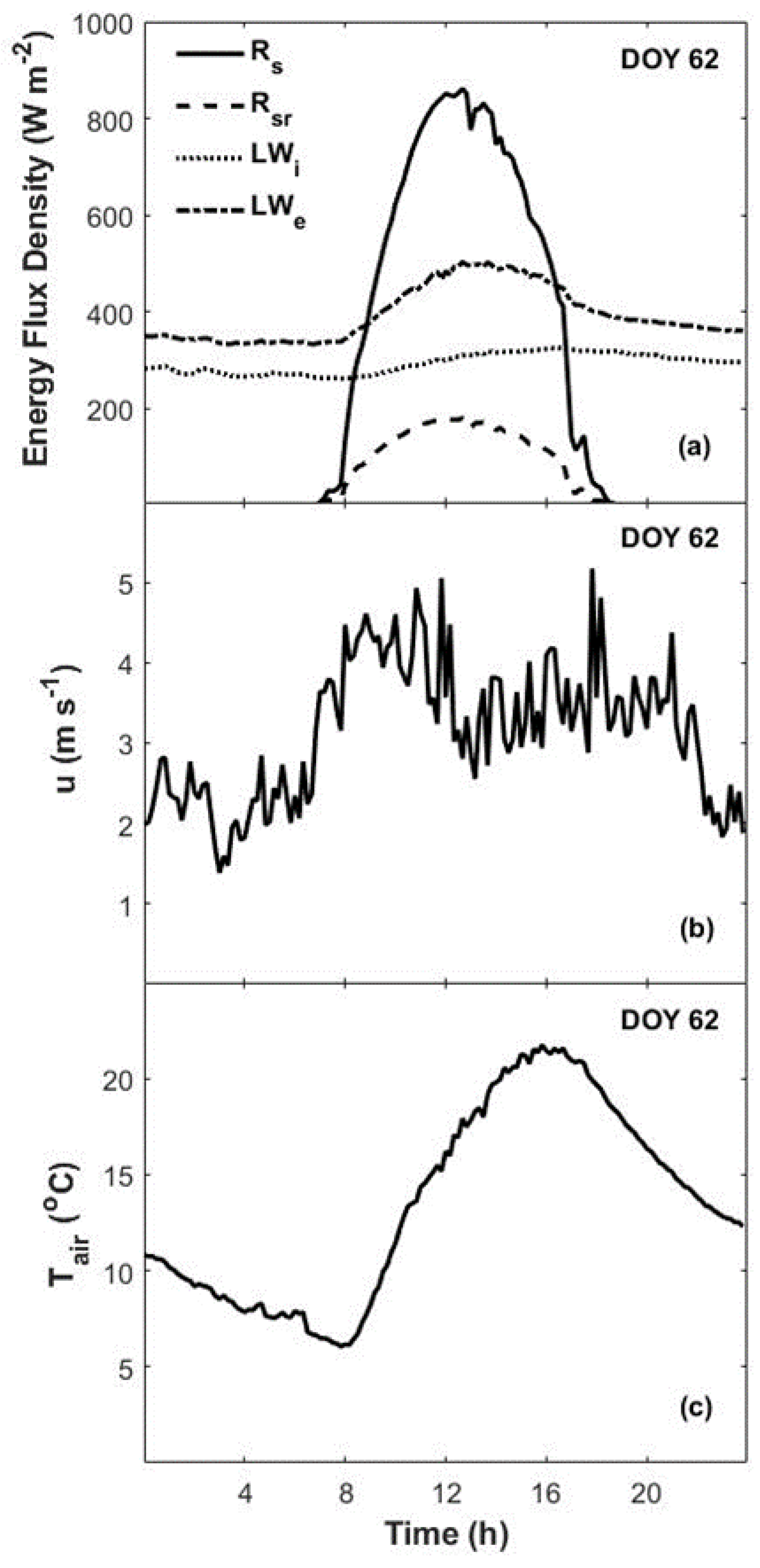
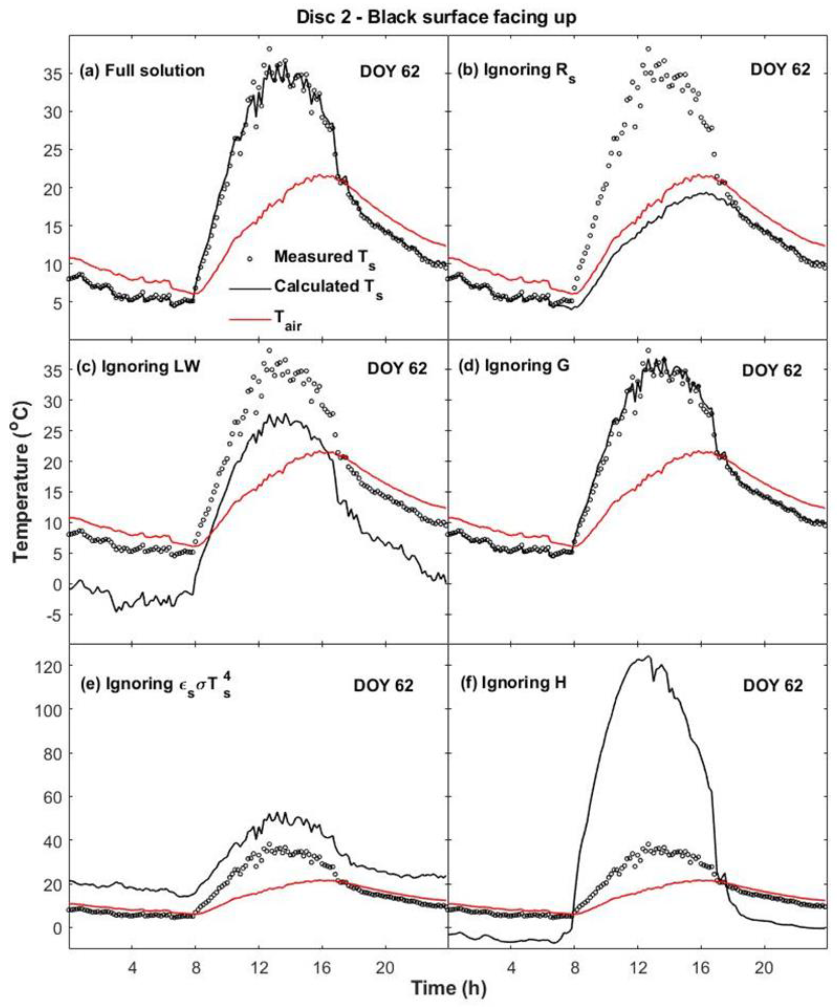
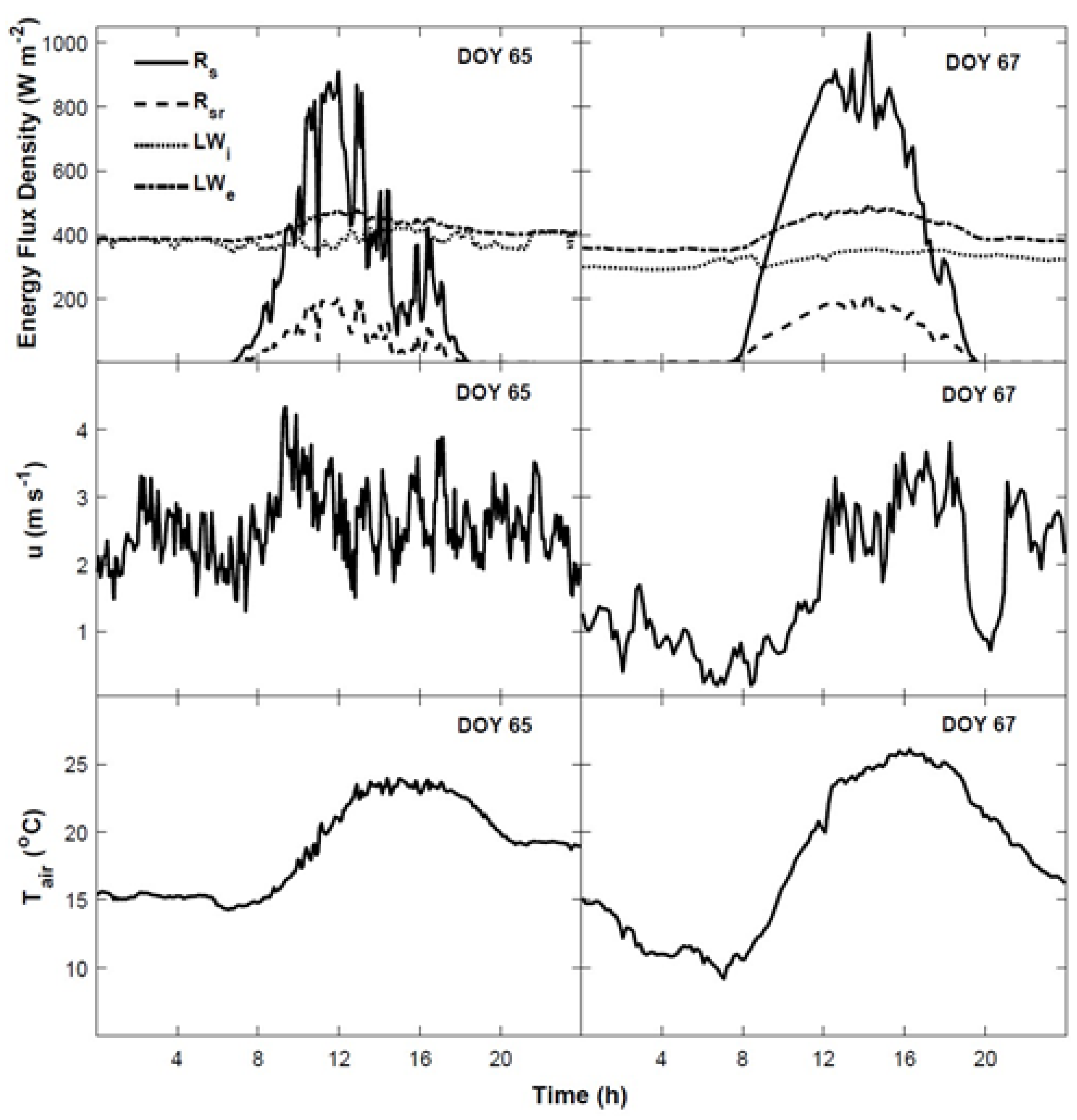
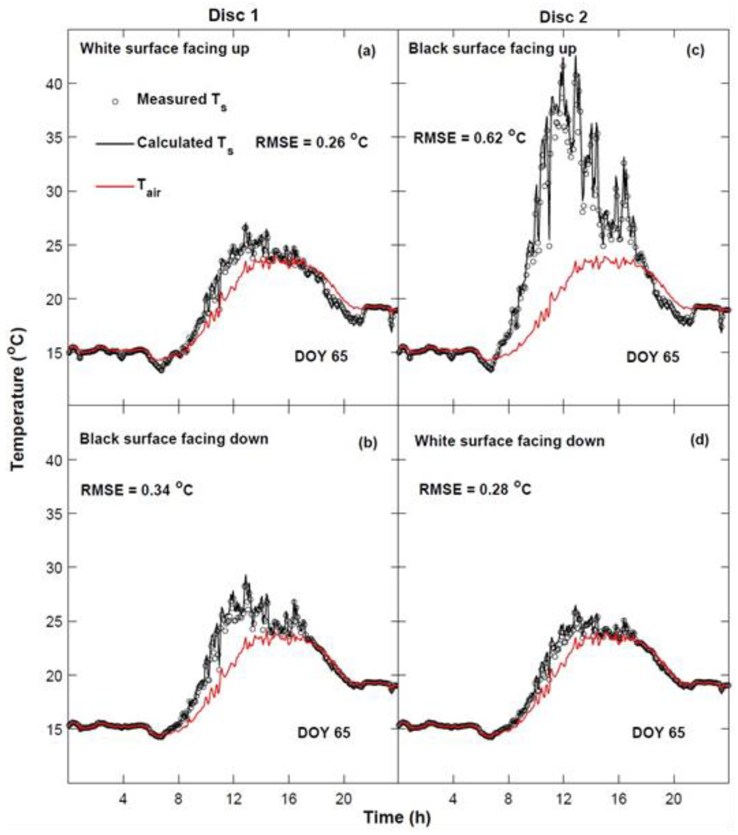
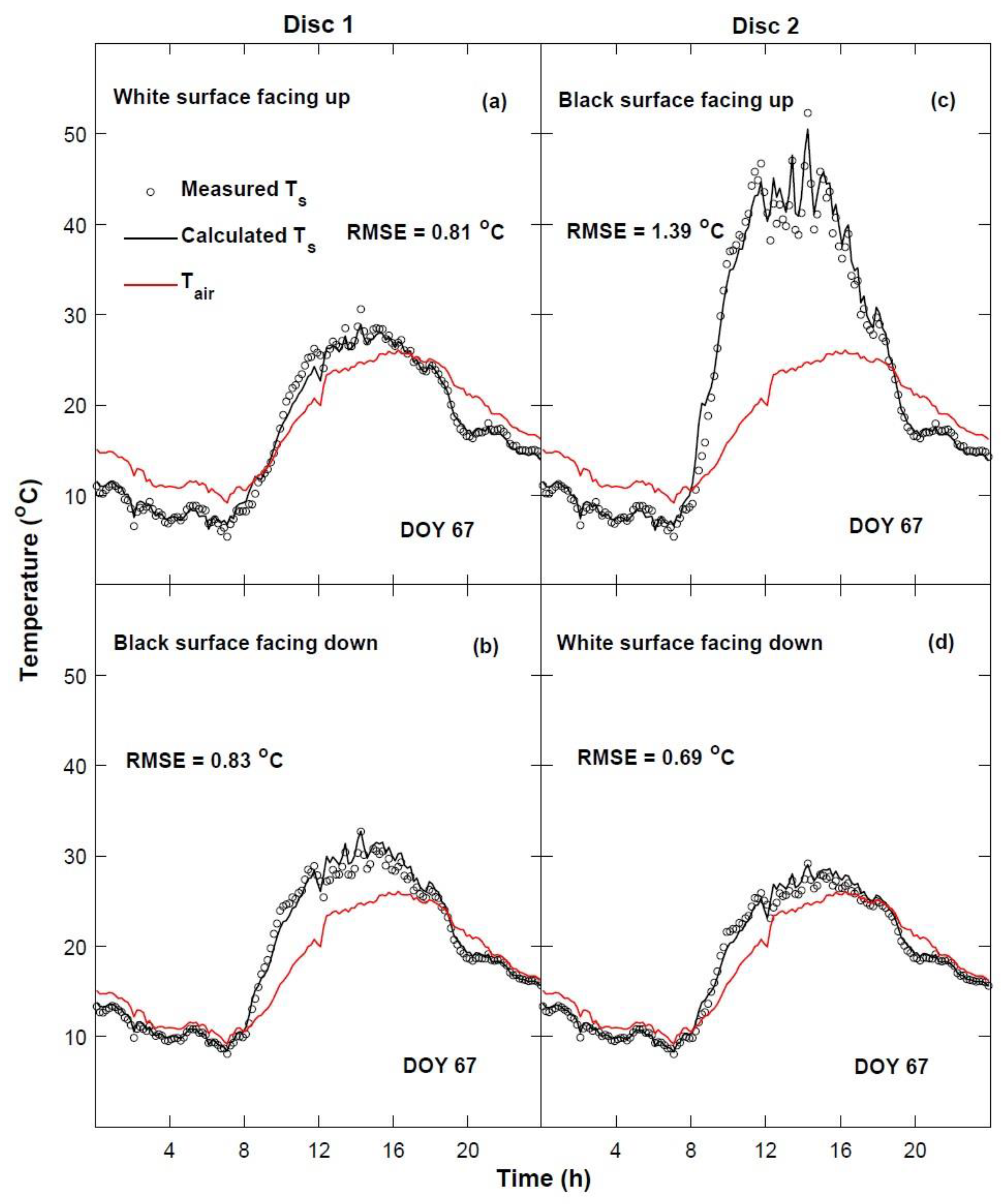
3. Results and Discussion

Environmental conditions on days of year (DOY) 65 and 67 are presented in Figure 4. DOY 65 was a windy day with cloudy skies. Total R_s, R_sr, LW_i, and LW_e were 14 MJ m⁻², 3 MJ m⁻², 33 MJ m⁻², and 36 MJ m⁻², respectively. Average T_air was 19 °C and average u was 3 m s⁻¹. DOY 67 was a clear day with low wind speeds. Total R_s, R_sr, LW_i, and LW_e were 23 MJ m⁻², 5 MJ m⁻², 28 MJ m⁻², and 35 MJ m⁻², respectively. Average T_air was 18 °C and average u was 2 m s⁻¹. Differences in LW_i between DOY 65 and 67 are due to the effect of clouds, which increased the emissivity of the atmosphere. This was evident during the night on DOY 65, when the longwave balance was close to zero, whereas on DOY 67 it was negative, indicating that the surface underneath the discs was cooling through the emission of longwave radiation.

In general, a good agreement was observed between calculated and measured values for the surfaces of the discs on DOY 65 and 67 (Figure 5 and Figure 6). On DOY 65 deviations from measured values for disc 1 (white surface facing up and black surface facing down), were on average 0.2 °C ± 0.1 °C for the white surface (Figure 5a) and 0.3 °C ± 0.2 °C for the black surface (Figure 5b), whereas on DOY 67 deviations for the white and black surfaces were 0.6 °C ± 0.6 °C and 0.6 °C ± 0.5 °C, respectively (Figure 6a,b). For disc 2 (black surface facing up and white surface facing down) deviations from measured values on DOY 65 were on average 0.4 °C ± 0.4 °C and 0.2°C ± 0.2 °C for the black and white surfaces (Figure 5c,d), respectively, whereas on DOY 67 deviations for the black and white surfaces were 1.0 °C ± 0.9 °C and 0.5 °C ± 0.5 °C, respectively (Figure 6c,d). Largest deviations from measured values occurred in the early morning hours of DOY 67 for the upper surface of disc 2 (black), when the calculated temperature was higher than the measured values by 5 °C (Figure 6c). This discrepancy is probably explained by dew evaporation from the surface of the disc, since latent heat flux was not accounted for in the energy balance calculations.

During daytime the surfaces of both discs were warmer than air on both DOY 65 and 67 (Figure 5 and Figure 6). As expected, the upper surface of disc 2 (black) had the highest temperature of all on both DOY 65 and 67 (Figure 5c and Figure 6c). Peak surface temperature on DOY 65 and 67 for the upper surface of disc 2 was 42 °C and 52 °C, respectively (Figure 5c and Figure 6c). That difference was due to higher solar irradiance and lower wind speeds on DOY 67 (Figure 4). Peak daytime surface–air temperature differences for the upper surfaces of disc 1 (white) and disc 2 (black) on DOY 65 were 4 °C and 20 °C (Figure 5a,c), respectively, whereas on DOY 67 it was 4 °C and 26 °C, respectively (Figure 6a,c). This highlights the effect of the differences in albedo on surface temperature of non-evaporating surfaces. It is interesting to note that during daytime on both DOY 65 and 67, the lower surface of disc 1 (black) was warmer than its upper surface (white) (Figure 5a,b and Figure 6a,b). During the night, surfaces of both discs remained well coupled to air temperature on DOY 65 (Figure 5). While the lower surfaces of both discs were close to air temperature during the night on DOY 67 (Figure 6b,d), the upper surfaces cooled about 3 °C below air temperature (Figure 6a,c). That is explained by the lower emissive power of the atmosphere on DOY 67 (cloudless skies) and highlights the importance of longwave radiation on the surface energy balance of objects at night (Figure 4).

Components of the energy balance of the discs on DOY 65 and 67 are shown in Figure 7 and Figure 8. Energy fluxes for black and white surfaces showed contrasting differences on both days. Black surfaces had higher energy fluxes than white surfaces during the daytime (Figure 7 and Figure 8), which was mainly due to albedo differences (Figure 2). The upper surface of disc 2 (black) had appreciably high R_n and H on both days (Figure 7b and Figure 8b), and that was mainly due its lower albedo. It is interesting to note that G was of equal magnitude, but of opposite sign for the black and white surfaces during daytime (Figure 7 and Figure 8). Therefore, R_n and G were energy sources for white surfaces and all energy was dissipated in the form of H, whereas for the black surfaces R_n was dissipated as H and G during daytime (Figure 7 and Figure 8). At night H was the main source of energy for the surfaces of both discs, which was dissipated mostly as R_n (Figure 7 and Figure 8). Differences in energy fluxes during the night between DOY 65 and DOY 67 are mainly due to higher LW_i and wind speeds on DOY 65 (Figure 4), which allowed both surfaces of the discs to be well coupled to air temperature. The magnitude of R_n and H for the upper surfaces of the discs during the night on DOY 65 and 67 is worth noting (Figure 7 and Figure 8). On DOY 65 average R_n and H for the upper surfaces of the discs were −18 W m⁻² and 17 W m⁻², respectively, whereas on DOY 67 it was −59 W m⁻² and 55 W m⁻², respectively (Figure 7 and Figure 8). Greater energy fluxes on DOY 67 are due lower LW_i (Figure 4), which allowed greater radiative cooling of the surfaces facing the sky. This highlights the importance of H in regulating surface temperature of objects that face the sky at night, which could otherwise cool to appreciably low temperatures due to the emission of longwave radiation.

The consequences of ignoring components of the energy balance equation on the calculation of T_s for the black surface of disc 2 (upper) are shown for the conditions of DOY 62 (Figure 9). DOY 62 was a windy day with clear skies. Total R_s, R_sr, LW_i, and LW_e were 21 MJ m⁻², 5 MJ m⁻², 25 MJ m⁻², and 34 MJ m⁻², respectively. Average T_air was 13 °C and average u was 3 m s⁻¹ (Figure 9). Errors in calculated T_s are shown in Figure 10. Complete solution of the energy balance equation showed good agreement with measured values (Figure 10a). When R_s was neglected (equivalent to setting albedo = 1), calculated T_s fell well below measured values and about 2 °C below air temperature during daytime (Figure 10b). Neglecting LW radiation input decreased calculated T_s during the daytime and at night (Figure 10c). It is interesting to note that during the night, calculated T_s reached a minimum of −5 °C, indicating the importance of incoming longwave radiation from the sky in regulating the temperature of objects at night (Figure 10c). As expected, calculated T_s increased when thermal emission is ignored as means of energy dissipation (Figure 10e). Calculated T_s was about 15 °C greater than measured values during the course of the day (Figure 10e). When H was neglected, calculated T_s was lower than measured values at night and appreciably higher than measured values during the day (Figure 10f). During the day, differences between measured and calculated values were substantial and followed closely the pattern of R_s (Figure 10f). Peak differences between measured and calculated values reached 92 °C, which indicates that convection was the primary mode of energy transfer during daytime (Figure 10f). The greatest difference between measured and calculated T_s at night was 12 °C, indicating the importance of convection in transporting energy towards the disc surface at night (Figure 10f). Ignoring conduction had a small effect on the calculations (Figure 10d). That was due to the low thermal conductivity of the foam material we used, which was effective in suppressing heat transfer between the surfaces of the disc.

4. Questions to Students

The following questions can be posed to students in order to stimulate discussions about how changing certain environmental variables and/or disc properties would influence the temperature of the disc:

• Would you expect to see higher surface temperatures under sunny or cloudy conditions?
• Would you expect to see higher surface temperatures under high or low wind speeds?
• If instead of parallel to the surface, the disc was mounted in a way such that it was perpendicular to the surface with its black surface facing west and its white surface facing east, during what part of the day would you expect to see the peak temperature of the black surface? What about for the white surface?
• How paints of different colors (different albedos) would affect the temperature of the disc?
• How paints of different emissivities would affect the temperature of the disc?
• How different diameters would affect the temperature of the disc?

5. Summary and Conclusions

We described the construction of a simple domeless net radiometer that can be used in laboratory activities in environmental physics courses. Measured and calculated surface temperatures showed good agreement under different environmental conditions. The data we presented were intended to show how the status of environmental variables and surface properties interact to regulate the surface temperature of objects. With the activity here proposed, students are expected to develop a deeper understanding of environmental physics theory, as well as gain some experience and practical skills in working with environmental sensors, programming data acquisition systems, and analyzing data. The questions posed to students are intended to stimulate them to think about how the conditions imposed by the physical environment determines the range of temperatures that are commonly observed in nature. It is hoped that the experience gained with this activity will benefit students by stimulating their creativity, as well as developing their analytical and problem-solving skills.

References

1. Campbell, G.S.; Norman, J.M. An Introduction to Environmental Biophysics, 2nd ed.; Springer: New York, NY, USA, 1998. [Google Scholar]
2. Monteith, J.L.; Unsworth, M.H. Principles of Environmental Physics, 4th ed.; Academic Press: London, UK, 2013. [Google Scholar]
3. Suomi, V.E.; Franssila, M.; Islitzer, N.F. An Improved Net-Radiation Instrument. J. Atmos. Sci. 1954, 11, 276–282. [Google Scholar] [CrossRef] [Green Version]
4. Suomi, V.E.; Kuhn, P.M. An Economical Net Radiometer. Tellus 1958, 10, 160–163. [Google Scholar] [CrossRef]
5. Fritschen, L.J.; van Wijk, W.R. Use of an Economical Thermal Transducer as a Net Radiometer. Bull. Am. Meteorol. Soc. 1959, 40, 291–294. [Google Scholar] [CrossRef]
6. Fritschen, L.J. Construction and Calibration Details of the Thermal-Transducer Type Net Radiometer. Bull. Am. Meteorol. Soc. 1959, 41, 180–183. [Google Scholar] [CrossRef] [Green Version]
7. Funk, J.P. Improved Polythene-Shielded Net Radiometer. J. Sci. Instrum. 1959, 36, 267–270. [Google Scholar] [CrossRef]
8. Tanner, C.B.; Businger, J.A.; Kuhn, P.M. The Economical Net Radiometer. J. Geo. Res. 1960, 65, 3657–3667. [Google Scholar] [CrossRef]
9. Funk, J.P. A Net Radiometer Designed for Optimum Sensitivity and a Ribbon Thermopile Used in a Miniaturized Version. J. Geo. Res. 1962, 67, 2753–2760. [Google Scholar] [CrossRef]
10. Fritschen, L.J. Construction and Evaluation of a Miniature Net Radiometer. J. Appl. Meteorol. 1963, 2, 165–172. [Google Scholar] [CrossRef] [Green Version]
11. Campbell, G.S.; Ashcroft, G.L.; Taylor, S.A. Thermistor Sensor for the Miniature Net Radiometer. J. Appl. Meteorol. 1964, 3, 640–642. [Google Scholar] [CrossRef] [Green Version]
12. Fritschen, L.J. Miniature Net Radiometer Improvements. J. Appl. Meteorol. 1965, 4, 528–532. [Google Scholar] [CrossRef]
13. Norman, J.M.; Blad, B.L.; Baker, D.G. Rain Correction Modification for a Non-Shielded Net Radiometer. J. Appl. Meteorol. 1966, 5, 730–733. [Google Scholar] [CrossRef] [Green Version]
14. Fritschen, L.J.; Gay, L.W. Environmental Instrumentation; Springer: New York, NY, USA, 1979. [Google Scholar]
15. Tanner, C.B. Basic Instrumentation and Measurements for Plant Environment and Micrometeorology; Soils Bulletin 6; University of Wisconsin: Madison, WI, USA, 1963. [Google Scholar]
16. Perrier, A. Leaf Temperature Measurement. In Plant Photosynthetic Production, Manual of Methods; Sestak, Z., Catsky, J., Jarvis, P.G., Eds.; W. Junk: The Hague, The Netherlands, 1971; pp. 632–669. [Google Scholar]
17. Bell, C.J.; Rose, D.A. The Measurement of Temperature. In Instrumentation for Environmental Physiology; Marshall, B., Woodward, F.I., Eds.; Cambridge University Press: Cambridge, UK, 1985; pp. 79–95. [Google Scholar]
18. Schooley, J.F. Thermometry; CRC Press: Boca Raton, FL, USA, 1986. [Google Scholar]
19. Ehleringer, J.R. Temperature and Energy Budgets. In Plant Physiological Ecology, Field Methods and Instrumentation; Pearcy, R.W., Ehleringer, J., Mooney, H.A., Rundel, P.W., Eds.; Kluwer Academic Publishers: Boston, MA, USA, 1989; pp. 117–134. [Google Scholar]
20. American Society for Testing and Materials. Manual on the Use of Thermocouples in Temperature Measurement, 4th ed.; ASTM: Philadelphia, PA, USA, 1993. [Google Scholar]
21. Brock, F.V.; Richardson, S.J. Meteorological Measurement Systems; Oxford University Press: New York, NY, USA, 2001. [Google Scholar]
22. McInnes, K.J. Temperature. In Methods of Soil Analysis, Part 4, Physical Methods; Topp, G.C., Dane, J.H., Eds.; SSSA: Madison, WI, USA, 2002; pp. 1183–1199. [Google Scholar]
23. Novak, M.D. Soil Temperature. In Micrometeorology in Agricultural Systems; Hatfield, J.L., Baker, J.M., Eds.; ASA-CSSA-SSSA: Madison, WI, USA, 2005; pp. 105–129. [Google Scholar]
24. Harrison, R.G. Meteorological Instruments and Instrumentation; John Wiley & Sons: Oxford, UK, 2015. [Google Scholar]
25. Slatyer, R.O.; McIIroy, I.C. Practical Microclimatology; CSIRO Plant Industry Division: Canberra, Australia, 1961. [Google Scholar]
26. Woodward, F.I.; Sheehy, J.E. Principles and Measurements in Environmental Biology; Butterworths: Boston, MA, USA, 1983. [Google Scholar]
Figure 1. Diagram showing thermocouple arrangements for surface temperature measurement. When arranged in (A) series thermocouples form a thermopile, when arranged in (B) parallel swamping resistors are necessary.
Atmosphere 12 01620 g001
Figure 2. Spectral reflectivity [ρ(λ)] of the white and black paints used to construct the discs.
Atmosphere 12 01620 g002
Figure 3. Discs built by students as part of their class project.; (a) close-up picture of a disc with its upper surface painted black and (b) picture of discs with upper surfaces coated with black and white paint. Discs were set up above a turf grass field for the class activity.
Atmosphere 12 01620 g003
Figure 4. Environmental conditions on days of year (DOY) 65 and 67. Solar irradiance (Rs), reflected solar irradiance (Rsr), incoming longwave sky radiation (LWi), emitted longwave radiation by the surface underneath the discs (LWe), wind speed (u), and air temperature (Tair) were measured at the height of the discs.
Atmosphere 12 01620 g004
Figure 5. Calculated and measured surface temperature of the discs on day of year (DOY) 65. Disc 1 had its upper surface painted white (a) and its lower surface painted black (b), whereas Disc 2 was the opposite (c,d). Deviation between measured and calculated values for each surface is given by the root mean square error (RMSE).
Atmosphere 12 01620 g005
Figure 6. Calculated and measured surface temperature of the discs on day of year (DOY) 67. Disc 1 had its upper surface painted white (a) and its lower surface painted black (b), whereas Disc 2 was the opposite (c,d). Deviation between measured and calculated values for each surface is given by the root mean square error (RMSE).
Atmosphere 12 01620 g006
Figure 7. Energy balance components for (a) Disc 1 and (b) Disc 2 on day of year (DOY) 65. Sign convection dictates that energy fluxes toward the surfaces of the disc are positive and fluxes away from the surfaces are negative.
Atmosphere 12 01620 g007
Figure 8. Energy balance components for (a) Disc 1 and (b) Disc 2 on day of year (DOY) 67. Sign convection dictates that energy fluxes toward the surfaces of the disc are positive and fluxes away from the surfaces are negative.
Atmosphere 12 01620 g008
Figure 9. Environmental conditions on day of year (DOY) 62. (a) Solar irradiance (Rs), reflected solar irradiance (Rsr), incoming longwave sky radiation (LWi), emitted longwave radiation by the surface underneath the discs (LWe), (b) wind speed (u), and (c) air temperature (Tair) were measured at the height of the discs.
Atmosphere 12 01620 g009
Figure 10. Calculated and measured temperature of the upper surface (black) of disc 2 on day of year (DOY) 62. Complete solution of the energy balance equation is shown in (a). Calculations are intended to show the errors in temperature estimation by neglecting: (b) solar irradiance (Rs), (c) longwave sky radiation (LW), (d) sensible heat flux by conduction (G), (e) emitted thermal radiation (εsσTs4), and (f) sensible heat flux by convection (H).
Atmosphere 12 01620 g010
Publisher’s Note: MDPI stays neutral with regard to jurisdictional claims in published maps and institutional affiliations.