The Relationship between Clouds Containing Multiple Layers 7.5–30 m Thick and Surface Weather Conditions

Abstract

Previous studies have identified finely laminated, or layered, features within Arctic clouds. This study focuses on quasi-horizontal layers that are 7.5 to 30 m thick, within clouds from 0 to 5 km altitude. No pre-selection for any particular cloud types was made prior to the identification of laminations. We capitalize on the 4-year measurement record available from Eureka, Nunavut (79.6${}^{\circ }$ N, 85.6${}^{\circ }$ W), using the Canadian Network for the Detection of Atmospheric Composition Change (CANDAC) Rayleigh–Mie–Raman Lidar (CRL; 1 min, 7.5 m resolution). Laminated features are identified on 18% of all days, from 2016–2019. Their presence is conclusively excluded on 12% of days. March, April, and May have a higher measurement cadence and show laminations on 41% of days. Individual months show laminations on up to 50% of days. Our results suggest that laminations are not rare phenomena at Eureka. To determine laminations’ likely contribution to Arctic weather and climate, local weather reports were obtained from the nearby Environment and Climate Change Canada (ECCC) weather station. Days with laminated clouds are strongly correlated with precipitating snow (r = 0.63), while days with non-laminated clouds (r = −0.40) and clear sky days (r = −0.43) are moderately anti-correlated with snow precipitation.

1. Introduction

Arctic clouds generally warm the surface by trapping and re-emitting upwelling infrared radiation; except in summer, when they contribute a slight cooling by emitting more radiation to space than they reflect back to the surface [1,2]. During the Arctic polar night, in the absence of incoming solar radiation, clouds can dominate the radiation budget; so, understanding their radiative impact is essential (e.g., [3,4,5,6]). Clouds also govern precipitation and, thus, are linked to local surface weather.

Inhomogeneities within clouds, and particularly the distribution of supercooled liquid water versus ice within mixed-phase clouds, are an important influence on weather and climate. The relative abundance of liquid versus ice controls the overall radiative balance via cloud optical depth effects [7]. Weather models depend on correct estimates of microphysical process rates for precipitation development, which themselves depend on measured vertical gradients of cloud properties [8]. The measurement of inhomogeneities, within clouds at all scales, is necessary.

Aircraft-based, multi-instrument case studies at Barrow, Alaska during the Mixed-Phase Arctic Cloud Experiment (M-PACE) have revealed mixed-phase clouds that contain layers of ice and liquid throughout the volume of the cloud [9,10,11,12]. These studies include detailed LiDAR (7.5 m × 2.5 s resolution), radar (45 m × 3–4 s resolution), and in-situ measurements. For Verlinde et al. [11], the total study duration was 12 h on 6 October 2004. During that period, up to six distinct liquid cloud layers were identified, each between 100–200 m thick, between 0 and 4.5 km altitude. Higher cloud layers precipitated ice into lower liquid layers, which usually contained drizzle. In this way, and via changes to the radiative heating profile, the layers interacted with one another over the cloud’s lifetime.

More recently, ground-based LiDAR measurements at Eureka, Nunavut, in the Canadian High Arctic, have reported similar internally-layered cloud phenomena at an order of magnitude smaller scale: 10s of meters per layer. Layers 100–200 m, as seen by Verlinde et al. [11], are also seen at Eureka. These larger layers are not the topic of the present study, as we now focus on the new detections of the finer scale phenomena. Measurements from the Canadian Network for the Detection of Atmospheric Change (CANDAC) Rayleigh–Mie–Raman Lidar (CRL; 7.5 m × 1 min resolution) showed that clouds at Eureka can contain numerous fine, vertically-stacked layers varying in size, down to at least as small as the resolution of the LiDAR, 7.5 m [13]. These are referred to as “laminations” in [13] and the present study. In 2019, McCullough et al. [13] carried out detailed case studies over 4 days with lamination-containing clouds. The laminations are clearly visible to the eye in plots of 532 nm range-scaled backscatter signal. For the McCullough et al. [13] case studies, CRL’s Rayleigh elastic measurements at 355 nm and 532 nm, the colour ratio between these signals, and the 532 nm linear depolarization ratio were all employed. Radiosonde measurements of temperature, relative humidity, and wind were used to support the case study investigation. The laminations are associated with thermal/convective stability. This combination provided insight as to the nature of the laminated features. Layers with high backscatter signals are often (but not always) associated with low depolarization; hence, these are interpreted to be liquid layers. Oriented plate ice particles is another possible interpretation. The between-layer properties have lower backscatter and higher depolarization, in general, and are interpreted to be randomly-oriented ice. Aerosols were also considered as a between-layers explanation, but these signals are very much higher than the signals returned from equivalent altitudes outside the cloud. The most likely explanation for the laminations is layers of liquid droplets alternating with layers of ice particles. Laminated clouds were shown to exist in at minimum winter, spring, and summer. Vertical variation within clouds at the 10s of metres scale had, prior to McCullough et al. [13], not been extensively reported in the literature (see literature search therein).

Given the importance of the vertical distribution of cloud particles within contiguous cloud volumes, we now carry on the work from McCullough et al. [13] and want to know how much of an impact the laminations are likely to have on the atmosphere at Eureka. Specifically, our goals are to: (1) quantify the number of days that have laminated clouds measured at Eureka, in order to place a lower limit on occurrence frequency of days with laminated clouds; (2) quantify the number of days whose measurements showed a definitive absence of laminated clouds, from which we can calculate a maximum possible occurrence frequency of days with laminated clouds (the interpretation of (1) and (2) will be supplemented by further classification of the days with unknown lamination status); we then aim to (3) test for correlations of days identified in (1) and (2) with surface weather reported at the co-located Eureka weather station. If we can quantify what kind of precipitation, or lack thereof, the laminated clouds are associated with, we can learn more about the conditions and microphysical processes occurring within the laminated cloud; this will (4) allow us to inform the direction of our future research on Arctic clouds.

We find that, over the 4-year study period of January 2016 through December 2019, days containing clouds with internal layering on the 7.5–30 m scale are not rare at Eureka. (1) Laminated features are identified on 18% of all days, indicating a lower limit on the observable occurrence frequency of days with laminated clouds. March, April, and May have a higher measurement cadence and show laminations on 41% of days. Individual months show laminations on up to 50% of days. (2) Laminated features are conclusively excluded on 12% of days in the four-year study period. (3) Days with laminated clouds are strongly correlated with precipitating snow (r = 0.63), while days with non-laminated clouds (r = −0.40) and clear sky days (r = −0.43) are moderately anti-correlated with snow precipitation. Correlations between days with laminated clouds and other weather types are far weaker. Therefore, (4) our future cloud research will be directed toward an understanding of the possible development of precipitating snow within laminated Arctic clouds.

2. Materials and Methods

2.1. Instrumentation

2.1.1. CRL Lidar

The Canadian Network for the Detection of Atmospheric Change (CANDAC) Rayleigh–Mie–Raman Lidar (CRL) is located at the Polar Environment Atmospheric Research Laboratory (PEARL; Eureka, Nunavut in the Canadian High Arctic, 79.6${}^{\circ }$ N, 85.6${}^{\circ }$ W).

CRL is a ground-based, zenith-pointing LiDAR. It contains two Nd: YAG lasers, one at 355 nm and the other at 532 nm, both operating at 10 Hz repetition rate. CRL has a 1-m Dal-Kirkham telescope and 8 measurement channels with photomultiplier tube detectors, some of which operate only in photon-counting mode, while the others make simultaneous photon-counting and analogue measurements [14,15,16]. The LiDAR has maximum 7.5 m vertical × 1 min time resolution. CRL can operate 24 h/day in any season, provided the winds are less than 20 knots and there is no precipitation buildup on the roof window. CRL is remotely operated from southern Canada.

While it is critical for this project that we be able to identify the laminated features, in order to count the days on which they occurred, it is conversely not necessary that we fully characterize each host cloud. Therefore, we use the CRL measurement set whose data has the best time and altitude coverage over the 4-year study period, which readily displays the laminated cloud features. The laminated features that we seek can be identified by eye in image plots of range-scaled 532 nm and/or 355 nm Rayleigh elastic backscattered signals. Based on operational constraints, CRL makes more measurements using the 532 nm Rayleigh elastic (non-depolarization) channel than any other. The 355 nm channel is not generally run during summer. At all times of year, the 355 nm laser has lower laser power than the 532 nm laser, resulting in a lower signal-to-noise ratio for the measurements. The 532 nm depolarization measurements require co-averaging to lower resolution and external calibrations, in order to be used. Depolarization data is also available for fewer days than is the 532 nm Rayleigh (non-depolarization) data. Therefore, only 532 nm range-scaled signal measurements from CRL are used in the present study.

Standard CRL processing routines were applied to the 532 nm measurements: saturation and deadtime correction, dark counts removal, background subtraction, and gluing of the photon-counting and analogue signals into a combined vertical profile for each minute. See, e.g., references [15,16] for full details about these procedures. The signals were multiplied by the square of the altitude of the returns. The resulting product is range-scaled signal in units of m${}^2$MHz.

2.1.2. Eureka Weather Station Meteorological Reports

Publicly available meteorological reports from Environment and Climate Change Canada (ECCC, formerly Environment Canada (EC)) Eureka Weather Station were used to investigate the weather conditions at the ground for all days during 2016–2019. The Eureka Weather Station instrument compound is located 180 m to the Southeast of the CRL Lidar, making the weather reports a co-located data set with CRL’s LiDAR measurements.

The ECCC weather data are recorded by human weather observers at Eureka. The data are generally reported hourly, with between 22 and 24 observations being made per day.

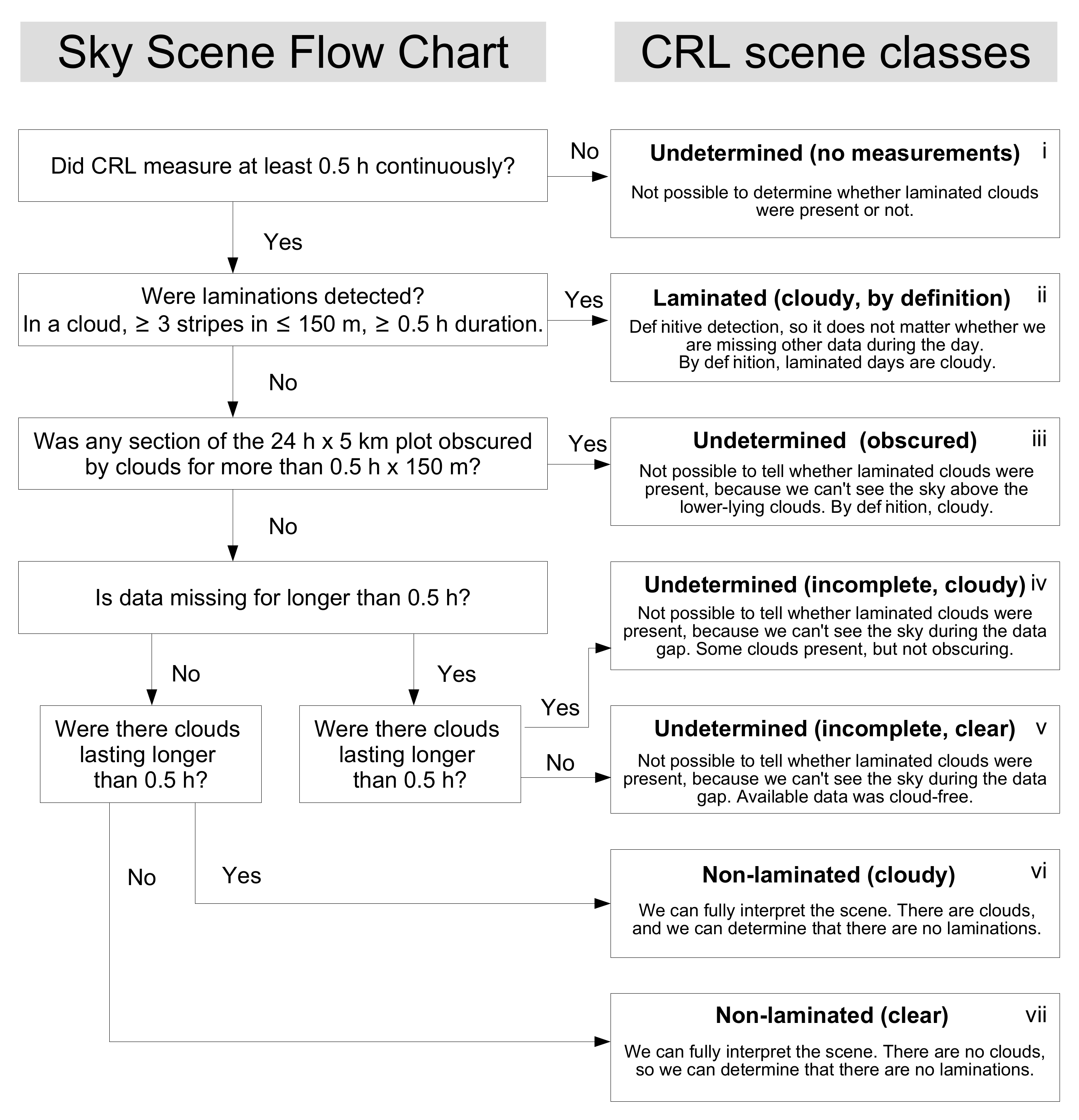
2.2. Method: Lidar Classification of Sky Scenes

A plot of CRL range-scaled 532 nm signal was produced for each 24 h UTC day from 0 to 5 km altitude at the measurement resolution (no further vertical integration). An example is given in Figure 1a. The classifier (human) was free to adjust the colour scale, aspect ratio, and zoom of each plot as they wished throughout the classification procedure. Shupe et al. [17] have shown that the annual mean lowest cloud bottoms at Eureka were at 1.75 km altitude, while the mean highest cloud tops were at 4.5 km, exceeding 5 km only in August. Therefore, the altitude range used in the CRL study, up to 5 km, is deemed sufficient to encompass most clouds at Eureka.

Each daily plot was classified according to the flow chart in Figure 2. The overall categories are:

• Laminated (the day contains at least one cloud with at least one detection of layered features meeting the criteria in Figure 2).
• Non-laminated (the day clearly contains no layered features within any clouds, which may or may not be present; the entire day is measured with the LiDAR).
• Undetermined (no clouds with qualifying layered features were measured by CRL; however, due to measurement limitations, the presence of clouds containing laminated features on that day cannot be conclusively ruled out.)

These three categories are sufficient to determine the lower and upper bounds on the occurrence frequency of days containing laminated clouds at Eureka. The specific criteria are given below. Subcategories assist in interpreting the results.

We examined many examples of plots exhibiting such laminated morphology to ascertain the specific quantitative characteristics of the laminations and developed classification criteria based on these. Readers who wish to assess the robustness of the classification criteria should use the supplementary plots (and data files for reproducing the plots using any colour scheme) provided.

Each individual layer of the laminated features that we seek to identify within clouds is no more than 30 m thick. We determined that laminated features could be reliably identified if at least three high-backscatter layers were located above one another, with a low-backscatter layer of the same thickness between each. Thus, we seek sets of three high-backscatter layers within a 150 m vertical extent. We selected 0.5 h as the minimum duration of this condition, in order to qualify the detection of a laminated feature.

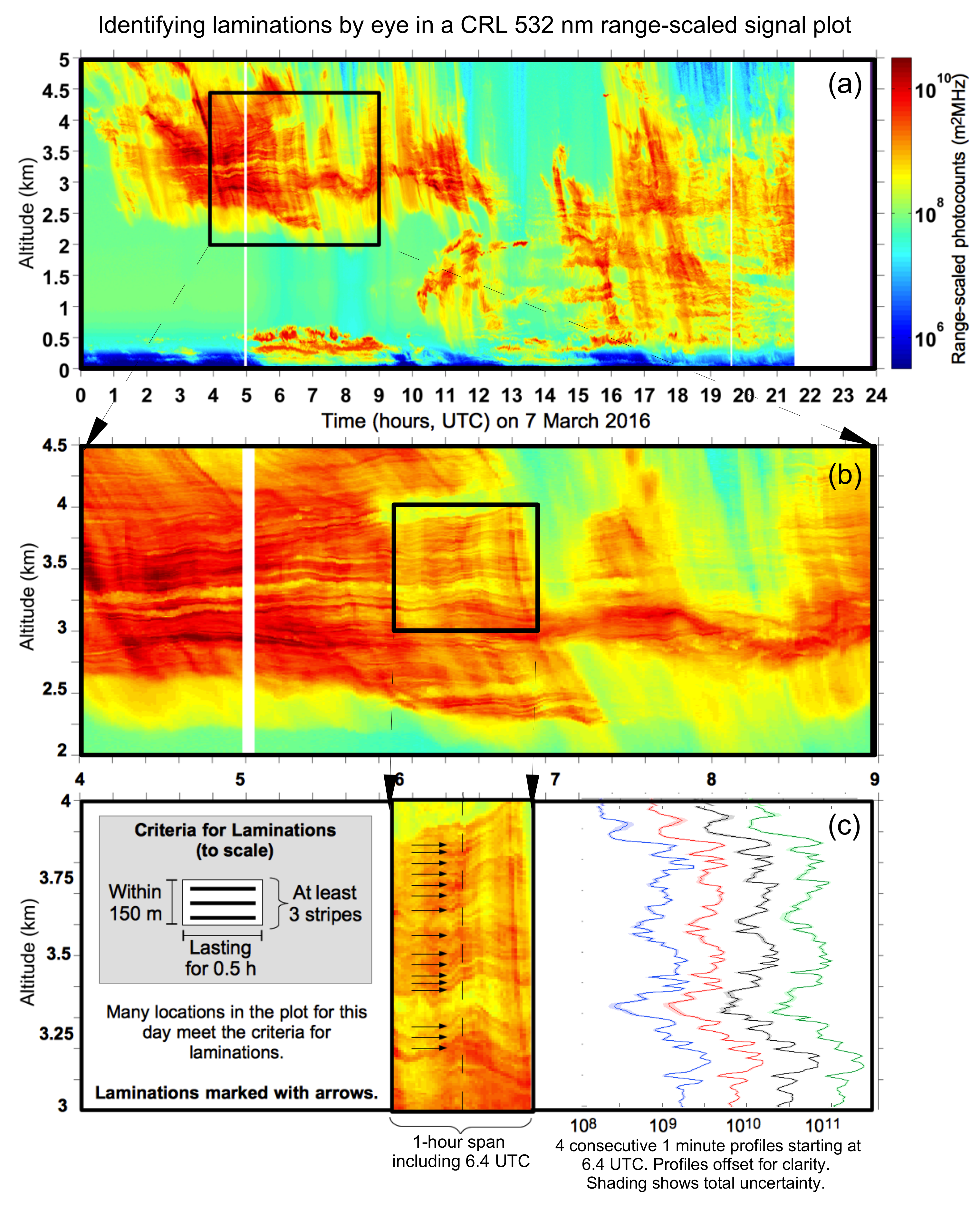
2.2.1. Identification Criteria for Laminated Classification

The criteria to classify a day as Laminated are:

• The laminated region occurs in a cloud and not only in a region of aerosol, dust, fog, etc. Defined edges of the cloud were visible, and the range-scaled signal value was higher than surrounding non-cloud values, by a factor of 10 or higher. Typical signal values are approximately ${10}^{8.5}$ m${}^2$MHz.
• There are a minimum of three quasi-horizontal, high-signal stripes, about equal in thickness, stacked one on top of the other, with maximum total extent of 150 m from the lower edge of the first stripe to the upper edge of the third stripe.
• The laminated condition lasts for a minimum duration of 0.5 h.

We found very few cases that were difficult to classify as either laminated or not. There were fewer than than 10 days in the 4 years dataset which had, for example, layered-type features that did not meet the extent criteria, or which lasted for shorter than the 0.5 h duration criterion. Therefore, we consider that the criteria appropriately encompasses the phenomenon that we are exploring.

Laminated days can be short in measurement duration. One laminated feature detection of 0.5 h is sufficient to identify the day as “Laminated”, even if there were no further LiDAR measurements made that day.

2.2.2. Identification Criteria for Non-Laminated Classification

The Non-laminated class identifies days for which there is a definitive absence of laminations. In order to state that there were no laminated clouds present in the atmosphere for a particular day, we must be able to fully discern all features for that entire 24 h × 5 km day in the CRL data and find no instances of laminated clouds therein. There is a tolerance for missing and/or obscured data for less than 0.5 h, because any laminations would need to have endured at least that length of time, in order to be identified according to our criteria.

The subdivision into Non-laminated (cloudy) and Non-laminated (clear) is made according to whether there is at least one cloud during the day with: signal values as in criterion (1) for Laminated; subtending at least 150 m in height; between 250 m and 5 km altitude; for at least 0.5 h.

2.2.3. Identification Criteria for Undetermined Classification

The remainder of the days will hold some uncertainty and are classified as Undetermined. We don’t see laminated clouds in the plot for these days, but it is possible that this is due to one or more contributions of measurement bias. For these days, there is a portion of the plot, of at least 150 m in height × 0.5 h, that is inaccessible to the LiDAR; in principle, a laminated feature could be obscured.

The Undetermined (obscured) category accounts for days during which clouds or other atmospheric phenomena extinguish the LiDAR beam, obscuring a contiguous region of the time-height plot above 250 m altitude for at least 150 m × 0.5 h. There is no restriction on the nature, location, or duration, of the obscuring phenomena themselves. Common examples are: fog, low altitude clouds, and clouds of high optical depth. Typical values to consider the LiDAR beam extinguished are signals less than ${10}^{6.5}$ m${}^2$MHz in the CRL data set.

Days with less than 0.5 h of CRL measurements are classified as Undetermined (no measurements). Days which contain 0.5 h–23.5 h of CRL measurements, and for which the entire column from 0–5 km is clearly visualized by the LiDAR (and which do not display laminated features), are classified as Undetermined (incomplete). These are sub-classified as Undetermined (incomplete, cloudy) if they contain at least one cloud large enough to host laminations and Undetermined (incomplete, clear) if all available data is cloud-free.

2.3. Occurrence Frequency Calculations

Because of gaps in the dataset (due to equipment repairs, operator availability, inclement weather, etc.), it is not possible to produce a comprehensive climatology of the occurrence of laminated features. Instead, we calculate the frequency and monthly distribution of days containing laminated clouds throughout the year. This is expressed as a minimum observed frequency (days on which we have definite detections of laminations) and maximum possible occurrence frequency (days for which we cannot definitively exclude laminations). This provides conservative lower and upper bounds on the frequency with which laminated clouds appear at Eureka.

The occurrence frequency of days containing laminated clouds was calculated on a yearly and monthly basis, as well as for the entire 4-year period together. The total number of days per observation period, $N_{Tot}$, varies from 28 (non-leap year Februaries in monthly calculations) to 1461 for all days in the 4-year study. As every day is classified as Laminated, Non-laminated, or Undetermined, the sum of the number of days classified in each category ($N_{Lam}$, $N_{Non}$, and $N_{Und}$, respectively) also gives $N_{Tot}$: $N_{Tot}=N_{Lam}+N_{Non}+N_{Und}$. We calculate both a minimum observed frequency and maximum possible frequency, expressed as a percentage:

$$\begin{array}{ccc}\hfill f_{minobserved}& =& 100\%\times N_{Lam}/N_{Tot}\hfill \end{array}$$

(1)

$$\begin{array}{ccc}\hfill f_{maxpossible}& =& 100\%\times (N_{Tot}-N_{Non})/N_{Tot}\hfill \\ & =& 100\%\times (N_{Lam}+N_{Und})/N_{Tot}\hfill \end{array}$$

(2)

The maximum possible number of days on which the Eureka atmosphere could possibly have contained laminated clouds is equal to the total number of days in the time period of interest, less the number of days for which we can definitively state that there were no laminated clouds, $N_{Non}$. Equation (2) provides two equivalent ways to divide $N_{Non}$ by the total days in the study period and obtain the maximum possible occurrence frequency, $f_{maxpossible}$.

2.4. ECCC Weather Report Categorization Method

For each day of ECCC meteorological data, we identified a positive detection for any type of weather, which was reported at any time during that day, and non-detection for any weather that did not occur that day.

Table A1. Number of days during 2016–2019 on which each type of ECCC weather condition was reported for at least 1 h. The second column removes any days for which there were no CRL measurements.

ECCC Reported	Number of Days	CRL Measurement
Weather Name	Reported	Days Only
Snow	543	333
Snow Grains	5	2
Snow Pellets	3	3
Snow Showers	7	4
Moderate Snow	5	3
Moderate Snow Grains	1	1
Blowing Snow	285	148
Rain	124	65
Rain Showers	34	16
Moderate Rain	2	2
Drizzle	8	4
Freezing Drizzle	5	4
Freezing Rain	4	0
Ice Crystals	547	301
Fog	212	145
Freezing Fog	39	26
Smoke	1	0
Haze	1	0
Blowing Sand	1	1
Dust	2	1
Ice Pellet Showers	1	0
Ice Pellets	2	1
Clear	601	389
Mainly Clear	664	453
Cloudy	499	340
Mostly Cloudy	761	530
No Value	1447	906

in Appendix A gives all reported weather conditions for 2016–2019, and the number of days on which each was reported.

For analysis in this paper, we have grouped the ECCC standard weather observations into categories, as in

Table 1. ECCC reported weather conditions were grouped together for comparison in this paper.

Weather Category	ECCC Weather Conditions Included
Snow	snow, snow grains, snow pellets, snow showers,
	moderate snow, moderate snow grains
Blowing Snow	blowing snow
Rain	rain, rain showers, moderate rain, drizzle,
	freezing drizzle, freezing rain
Ice Crystals	ice crystals
Fog	fog
Freezing Fog	freezing fog
Excluded from study	blowing sand, clear, mainly clear, cloudy, mostly cloudy,
	dust, haze, ice pellets, ice pellet showers, smoke, no value

. For example, our “Snow” category includes ECCC weather conditions “snow”, “moderate snow”, etc.

Weather types reported for two or fewer days, between 2016–2019, are either included in one of the combined weather categories (e.g., “snow showers” in “Snow”) or excluded from consideration if they would have required making a new category of their own (e.g., “Smoke”).

“Clear or mainly clear” and “Cloudy or mostly cloudy” were also excluded from consideration in this paper. These categories are not reported for all hours in which these conditions occur; rather, they are reported only for observation hours during which no other reportable weather occurred (e.g., “Cloudy” would not be reported in addition to “Snow” for a particular hour, even though clouds are required to be present in order for the snowing condition to be reported by ECCC).

2.5. Correlation of Laminations with Weather Reports

In this investigation, we seek any correlation between laminated clouds and meteorological conditions at Eureka. Clear and cloudy non-laminated scenes are also tested for correlation.

Two limiting cases are sought for correlation results:

• The strict case, which only includes days for which we have definitive measurements in Laminated (class ii in Figure 2) and Non-laminated classes (vi, vii). All Undetermined days (i, iii, iv, v) are excluded from the strict correlation tests.
• The inclusive case, which additionally includes most Undetermined classes as though they were non-laminated (i.e. Laminated includes class ii, Non-laminated includes classes i, iii, iv, v, vi, vii). Days with no measurements (class i) remain excluded from consideration, even in the inclusive case.

These limiting cases allow us to check whether our criteria for rejecting the Undetermined days from consideration for the Non-laminated category are too strict and unduly inflating the correlation of Laminated days with certain types of reported weather. This is a concern because, according to the criteria in Section 2.2.1, Section 2.2.2 and Section 2.2.3, a day with up to 23.5 missing hours with laminations would be “Laminated”, while the same scene with no laminations would be “Undetermined (missing)”, rather than “Non-laminated”.

Pearson product-moment correlation coefficients, r, and the associated significance values, p, were calculated for the three CRL categories (Laminated, Non-laminated (cloudy), and Non-laminated (clear)), and our weather categories are listed in Table 1.

The Pearson’s r is expressed as the covariance of two random variables divided by the product of the standard deviation of each variable X and Y, as in: r $=cov(X,Y)/{\sigma }_X\ast {\sigma }_Y$. In the case of this study, X is the vector identifying the presence and non-presence of a particular CRL Lidar sky scene classification as a function of date, and Y is the vector identifying the presence or absence of an individual weather category as a function of date. The data was artificially dichotomized, as the presence of one weather category, for example, does not preclude the presence of any other weather category that day. Thirty-six sets of $X,Y$ values were examined.

The interpretation of r is discussed at length in [18] as being useful only in a relative sense; context is required to state whether a particular value of r is “small” or “large”. Thus, all r values reported here are only useful when compared with one another. The convention suggested by [18] is what we will follow when using qualitative descriptors in this paper: r $=0.1$ is small, r $=0.3$ is medium, and r $=0.5$ is large. We are working with a 95% (2$\sigma$) confidence interval, so we take r values having p $\le 0.05$ to be significant.

We use r to express how the behaviour of the local weather conditions from ECCC varies with LiDAR classifications.

In our study, daily results were compared. A certain type of weather may be noted for a particular day, but may not have occurred at the same time as the laminated clouds, nor lasted the entire day. Consequently, there will be some noise expected in the final result, and the correlations are, thus, intended as minimum correlation amplitudes in both the strict and inclusive cases outlined above. Tables of correlation coefficient r were colour-coded for ease of interpretation, in the style of a corrgram or correlogram.

3. Results

3.1. Yearly Classification of Sky Scenes

Figure 3 shows the yearly CRL scene classification, considering all days of all years from 2016 through 2019. Positively identified laminated days (Laminated; blue) are at the bottom of each bar in the plot. The height of these bars indicates the observed minimum occurrence frequency of days with laminated clouds, $f_{minobserved}$: 17%, 14%, 24%, and 19%, respectively, as indicated by the thick black “Minimum observed” line in the plot. Considering all 1461 days of the 4-year study period together, the observed minimum occurrence frequency is 18% of all days. Every individual year had at least 52 days (14% of the year) with lamination detections. Thus, laminated clouds are not infrequent features, nor are they particular to one specific year. The similarity between the results for the 4 individual years indicates that laminations are a recurring condition of the Eureka troposphere.

Days which have been positively identified as Non-laminated extend downward from the top of the plot (red and striped orange bar segments). This defines the location for the “Maximum possible” thick black line, at $f_{maxpossible}$ = 87%, 90%, 87%, and 86% for each of the years. The 4-year dataset had an overall maximum possible occurrence frequency of 88%, our measurements having conclusively demonstrated that 12% of days are Non-laminated.

Overall, approximately one-fifth of all days at Eureka, at minimum, are affected by laminated cloud features at the tens-of-meters scale.

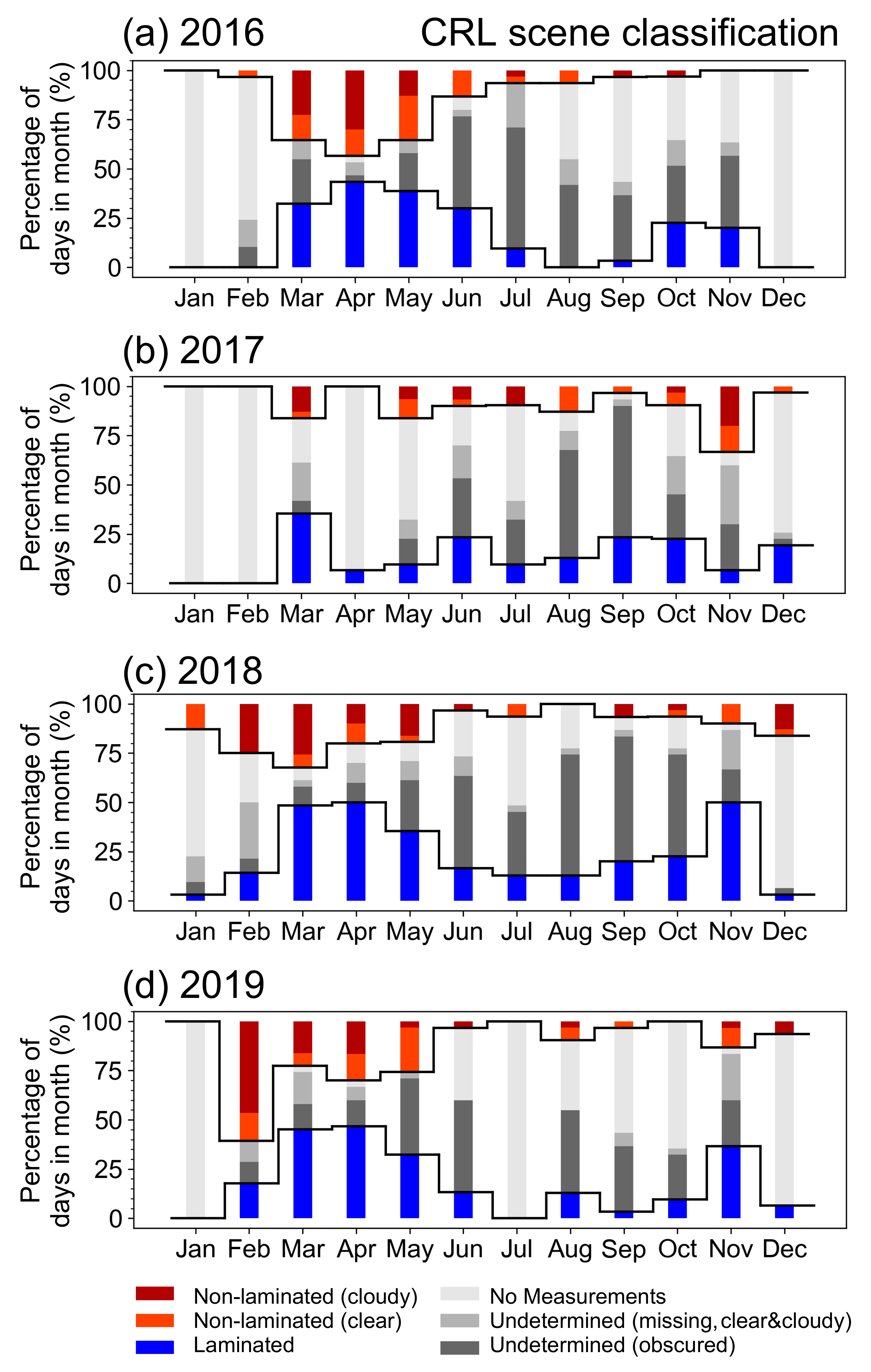
3.2. Monthly Classification of Sky Scenes

Figure 4 shows the same data as in Figure 3, broken down by month. The distribution of CRL measured days throughout the year is not consistent between years, nor throughout any single year. In particular, funding circumstances preclude the LiDAR from full operations during December and January, as well as at other times of year. Hot weather at Eureka precludes full operations during the summer. The LiDAR must be closed if laboratory temperatures exceed certain thresholds, if local wind speeds exceed 20 knots, and in cases of significant precipitation buildup on the roof window. Lidar maintenance must also be carried out, usually in February and October–November. Therefore, the Undetermined (no measurements) category times are not random. Consequently, the monthly distribution plots provide context for the yearly plots but do not serve as a detailed statistical study of the variation in the occurrence frequency of laminated clouds throughout the year. More beneficially, they indicate month-long time periods during which CRL has excellent measurement coverage. The majority of days during each of these months were classified as Laminated or Non-laminated (i.e., few Undetermined days). During such periods, the small range between observed lower and possible upper bounds on occurrence frequency leads to good precision for the estimate of the true lamination occurrence frequency at these times of year.

There was at least one detection of laminated clouds in every month, measured throughout the 4 years (the single exception being August 2016, with only two measurement days).

The strongest conclusions we are able to draw are those for the spring, when years 2016, 2018, and 2019 have excellent measurement coverage. March, April, and May have the highest number of measured days, principally because of the ACE/OSIRIS Arctic Validation Campaign, which occurs annually during polar sunrise (see for example: [19,20,21] and the references therein) and because the measurements tend to be easily continued following the campaign each year. During these months CRL was operating for more than 28 days per month, and most of these days had 24 h × 5 km sky scenes, which were interpretable as Laminated, Non-laminated (cloudy), or Non-laminated (clear). Few days during these times of year had measurements with undetermined classifications. We can be confident that CRL is getting an accurate picture of the sky.

For all four individual years, the March–May $f_{minobserved}$ were: 38%, 17%, 45%, and 41%. The $f_{maxpossible}$ were: 62%, 89%, 76%, and 74%. Excluding 2017 (which made few March-May measurements), the combined three year observed minimum laminated cloud occurrence frequency for March–May was 41%, and the possible maximum was 71%.

April 2016 is the individual month with the best precision (smallest number of undetermined days), i.e., $f_{minobserved}$ = 43%, and $f_{maxpossible}$ = 57% of days. April 2018 is the individual month with the highest relative number of observed laminated days: 50%. This is a clear indication that laminations in Arctic clouds at Eureka are an integral component of the atmosphere during the spring season.

June and July generally have measurements on more than half of the days per month, but most of these days result in undetermined categorizations. Frequent fog and cloud at low altitudes obscure the sky scene above on 80% of the measured summer days. This accounts for more than half of all summer days. Therefore, we cannot draw strong conclusions for these months.

August–October each year also contain many cloudy days that obscure parts of the sky scene at higher altitudes. For these months, we have positive lamination detections, which set an observational floor of 20% for all years together. If there are hidden laminated clouds above the optically thick fog and clouds, we may be under-counting lamination events, especially during summer and early fall. This is especially likely, given the high number of Undetermined (obscured) days (e.g. in August and September 2017 and August–October 2018.). The upper limits for August–October are all above 80%. The spread between lower and upper bounds indicates the poor precision available for these months.

November shows $f_{minobserved}$ = 28% for all years together (20%, 7%, 50%, and 37% of days in the month, for each year individually). Therefore, springtime is not the only time of year during which fully half of the days of the month may experience laminated clouds. The upper limit is less informative, due to the large number of Undetermined (obscured) days in November: $f_{minobserved}$ = 100%, 67%, 90%, and 87% of days in the month, for each year individually.

December, January, and most Februaries have zero to few CRL measurements measured days for CRL because of funding and operational constraints at PEARL. Therefore, although the percent of days with laminations in Figure 4 is a small number, it is based on so few measurements that it is not yet a particularly significant finding. February 2019 had good coverage and laminations on about 25% of all days. February 2016, 2017, and 2018, however, did not have sufficient measurement days to conclude whether this is a general feature of February at Eureka or whether 2019 is somehow different. February 2016 had only one measurement, February 2017 had zero, and for February 2018, there were unclassified days for more than 50% of the month. Better estimates of the monthly laminated cloud frequency would be possible with increased funding to operate CRL during the December to February period each year.

The 2017 dataset had fewer clearly classifiable days (Laminated, Non-laminated (clear), and Non-laminated (cloudy)) than any other year in the study. It is also missing a long series of data in the springtime months (e.g., April, with only two measurements days). While the measurements we have for 2017 do not contradict the overall conclusions we draw from 2016, 2018, and 2019, they are not on their own strong enough to explore in detail. Even September 2017, missing only one measurement day, is less than helpful—most measured days are obscured by low cloud.

Cloud laminations are present throughout the year in the troposphere at Eureka. Most examples have been identified in the spring and late fall, but they are not absent at any time of year. The 4 studied years are very similar to each other. From this, we infer that four years of measurements is an ample duration to act as a study period, when making more detailed investigations as to the nature of the laminations, as well as the types of macro- or micro-physical processes with which they may be correlated, as we test in Section 3.3.

3.3. Correlations of Laminated Features with Weather Conditions

The three sky scene classifications were compared with each of the six categories of ECCC weather data. The Pearson’s r correlation values were calculated as described Section 2.5, for both strict and inclusive criteria. Correlation scores can vary between $r=-1$ (complete anti-correlation) and $r=1$ (complete positive correlation). In Figure 5, stronger correlations are highlighted with darker shades of red or blue and significant values of r are in bold.

The correlation plots in Figure 5 give the results for 2016–2019 combined. The left panel (a) shows the version using the strict criteria: Laminated (class; ii), Non-laminated (cloudy; vi), and Non-laminated (clear; vii) all have their definitions, as described in Section 2.2.1, Section 2.2.2 and Section 2.2.3. No Undetermined days are included in this panel.

Laminated clouds have large positive correlations only with precipitating snow (snow category; r $=0.63$). Much smaller positive correlations are seen with rain, blowing snow, and fog. Other weather conditions did not have significant correlations with laminated clouds. Non-laminated cloudy days were negatively correlated, with medium strength, with snow (−0.37). Small correlations were seen with rain (negative) and ice crystals (positive). Non-laminated clear days also showed medium negative correlations with snow (−0.40). Small negative correlations were recorded with rain, blowing snow, ice crystals, and fog.

The right panel (b) has more inclusive criteria for the Non-laminated categories. All Undetermined days, which had at least 0.5 h of measurements, are here included in Non-laminated categories (equivalent to supposing that the LiDAR detected every case of laminated clouds that occurred in the atmosphere). Thus, Non-laminated (cloudy) additionally includes Undetermined (missing) days that contain clouds and all Undetermined (obscured) days, since these are, by definition, also cloudy. Non-laminated (clear) additionally includes Undetermined (missing) days that are clear. Panel (b) uses: Laminated (class; ii), Non-laminated (cloudy; iii, iv, vi), Non-laminated (clear; v, vii).

Using the inclusive criteria, the overall pattern of results is the same as for the strict criteria. Laminations are still most strongly correlated with snow (0.43) and more weakly correlated with other weather categories. Non-laminated (cloudy) shows small negative correlations with snow (−0.17), and Non-laminated (clear) shows medium negative correlations with snow (−0.31). The correlation strengths for the inclusive case are smaller in all cases than for the strict case, which makes sense, given our selection criteria. As for the strict case, the correlations between laminated clouds and snow, in particular, are both (1) stronger and (2) positive, as compared to the correlations between non-laminated categories and such weather, which is (1) weaker and (2) negative.

Figure 6 gives the same kinds of correlation plots as those presented in Figure 5, separated by year. The results show the same pattern year-by-year, as we find for the combined-years calculations. Panels a,b,c,d contain the strict criteria. Panels e,f,g,h have the inclusive criteria. An identical pattern is observed to that in Figure 5, i.e., the strongest positive correlations are between laminated clouds and snow. Negative correlations are between all non-laminated categories and snow. Other weather categories have some significant values, all of these other correlation values are smaller in amplitude than the snow correlation already mentioned.

For the individual years, particularly for the more inclusive criteria version (e–h), there are more insignificant correlation results than there are for the strict version (a–d) and combined-years versions (a and b). Nevertheless, all years, in every test, have results that support the overall pattern observed in Figure 5.

4. Discussion

4.1. Discussion of Sky Scene Classification

The first part of this investigation seeks to determine the frequency with which days containing laminated clouds occur at Eureka. Over the 4-year period, the observed minimum occurrence frequency is 18% of all days, and laminations are definitively not present in the atmosphere between 0 and 5 km on 12% of days. Days with laminations present are distributed throughout the entire year and are not confined to a single season.

Regarding the interpretation of these results, the minimum occurrence frequency of laminated clouds is reported, in the context of a relatively high number of unmeasured or otherwise undetermined days per year. We interpret the 18% occurrence frequency as a lower bound for the presence of laminations. The true occurrence rate of these features is likely to be higher.

Throughout this study, a single qualified detection of clouds (and/or laminations) during a particular day (according to Figure 2 and Section 2.2.1, Section 2.2.2 and Section 2.2.3) is sufficient to classify that day as “cloudy” (and/or “Laminated”). We intend these terms, in this context, to mean “the day is not entirely cloud-free” and “the day is not entirely free of laminated features”, respectively. Therefore, in no circumstance should “cloudy” days in this study be interpreted as being necessarily predominantly cloudy. Likewise, a “Laminated” day is not necessarily predominantly filled with laminated features. Often, clouds contain some portions that are laminated and others that are not.

As a consequence of the study methodology, it would be inappropriate to infer, for example, that the Eureka environment spends one-fifth of all time with laminated cloud conditions present. Works, such as [22], have produced climatologies, regarding the overall cloudiness of the Eureka atmosphere. We do not aim to reproduce these results, and our methodology reflects our different goals. As well, we are not comparing the relative occurrence of cloudy compared to cloud-free times at Eureka.

Instead, noting the frequency with which laminated features exist, in the manner we have chosen, is helpful for showing that laminations are not rare at Eureka. They occur at all times of year, and any particular day has at least an 18% chance of having a laminated cloud at some point during that day. They are an atmospheric feature worthy of study, and this provides confidence that the second half of our study, regarding correlation with weather, was worthwhile to pursue.

4.2. Discussion of Correlations with Precipitating Snow

The correlation analysis between CRL sky classifications and ECCC weather yielded the same results for both the combined 2016–2019 and individual years datasets, as well as for both strict and inclusive criteria used to identify non-laminated days. Precipitating snow is the individual type of weather most strongly correlated with laminated clouds. The correlations of precipitating snow, with all non-laminated categories, is negative. This is consistent with the finding from case studies in [13].

McCullough et al. [13] made a preliminary report of several cases of coincident laminated clouds and rain; however, the more quantitative analysis covering the full 4 year period indicates that only 2016 and 2019 had any significant correlations of rain with laminated clouds, which were small positive correlations and only significant when using the strict criteria for classification. Rain has more than one formation mechanism in clouds. Raindrops can form directly from water vapour (condensing droplets, conceivably from convective clouds with vertical mixing, in which case we would expect no persistent laminations). Rain can also form indirectly, from melting snowflakes—potentially from snowflakes formed inside and precipitating out of laminated clouds, which we have shown to be strongly correlated with precipitating snow. In this scenario, the snowflakes would be melted by the time they are measured by the ECCC weather station at ground level. This confounding variable may contribute to the small correlation of rain with cloud laminations in some years. Perhaps only certain kinds of raindrops, which have formed via specific processes, are correlated with laminated clouds. Adding more years’ data into this study might reveal more significant small correlations of rain with laminated clouds (or rule them out).

A different perspective on the correlation of rain with laminated clouds is possible if we are more interested in the formation of rain than we are in the properties of the laminated clouds themselves. Of the 81 days with rain in our study, 22 of them hosted laminations. The correlations with rain are lower than they are for precipitation snow using the method presented here; so, it is likely that the effect of laminated clouds on the year-round Eureka atmosphere is dominated via production or development of snow. However, during the short time of year, during which rain can form, rain event production may still be influenced by the presence of laminated clouds to some extent.

Snow and rain are formed in clouds, so it is not surprising that these forms of precipitation have significant negative correlation with clear/cloud-free sky conditions. More interestingly, snow was found to be significantly negatively correlated with non-laminated cloudy conditions. Precipitating snow is more likely to occur on a cloudy day if the clouds exhibit laminations than if the clouds are non-laminated. Rain is also more likely if the clouds are laminated, compared to if they are not, although to a much lesser degree. This points to formation mechanisms of snow, and perhaps rain as well, in relation to cloud appearance in high resolution LiDAR data. This contrast in correlation values between laminated and non-laminated clouds, in otherwise identical sky conditions (fully sensed up to 5 km for 24 h, with clouds visible), is a key result of this analysis. The precipitating snow is correlated with laminated clouds, and it is negatively correlated with non-laminated clouds. This finding leads to interesting questions regarding the types of the clouds that the laminations occupy. McCullough et al. [13] demonstrated, with depolarization measurements, that many of the laminated clouds are mixed-phase clouds.

We did not confine the present study strictly to mixed-phase clouds, due to practical limitations within the dataset. The 4-year dataset from CRL has 532 nm backscatter measurements for many more days than it has the depolarization measurements needed to confirm particle phase and, thus, to confirm whether a particular cloud is mixed-phase or not. Even so, it is likely that many of the cases identified in the present study are mixed-phase clouds. Every case studied in McCullough et al. [13] was a mixed-phase cloud - even the summer example. Climatologies have shown that Eureka, Nunavut (our study site) has a 25% annual average fraction of mixed-phase clouds [22]; therefore, a significant portion of the clouds measured in this paper are likely to belong to the mixed-phase class.

The small positive correlations of CRL sky scene classifications with blowing snow are much smaller than those with (precipitating) snow. Therefore, we conclude that precipitating snow is the dominant form of snow, in relation to laminations. One practical aspect of weather observation at Eureka station may allow the snow and blowing snow categories to become somewhat conflated. The weather conditions (snow, blowing snow, ice crystals, etc.) are reported using observations made at Eureka weather station, at 10 m above sea level. The wind speeds are recorded at the airport runway, which is 1.8 km to the Northeast and 73 m higher in elevation than the weather station’s instrument compound. Due to ECCC’s reporting criteria, blowing snow is not able to be reported when the wind speed is less than a minimum value. There is the possibility of a confounding variable in the blowing snow category arising from local wind speed. [13] established no relationship between laminated clouds and wind speed. Changes in the reporting methods may account for some of the relative increase in the number of blowing snow cases year-by-year.

Ice crystals, fog, and freezing fog show correlations that are only significant for some years with the CRL sky scenes. Ice crystals are better correlated with non-laminated (cloudy) skies than they are with laminated skies; perhaps this is because of the types of clouds included in the Non-laminated (cloudy) category. This category, even under the strict criteria named here, is actually quite inclusive, in terms of what kinds of clouds are required for “cloudy” and how small they can be. Future studies may wish to further restrict the qualifications that a particular cloud, or day, must reach, in order for the day to be classified as “cloudy”.

Micro-physical processes producing snow should be considered, in the context of laminations. Cloud particle phase classifications could be in error if a laminated cloud is measured only resolution coarser than the size of the laminations. Fine resolution may reveal alternating ice and water particles, based on alternating low backscatter (with high depolarization ratio) and high backscatter (with low depolarization ratio). As we see at Eureka, this can happen on at least 18% of all days throughout the year, as well as on at least 50% of days in certain months. At coarse resolution, analysis may erroneously show a smoother cloud, with a combination of mid-value backscatter and a mid-value depolarization ratio, neither of which are representative of any particles actually in the cloud. This could result in misleading interpretations, regarding microphysical processes which form, or act upon, the particles actually present in the cloud.

5. Conclusions

Laminated cloud features, containing individual layers 7.5–30 m thick, within Arctic clouds occur often at Eureka, Nunavut, as determined by a 4-year, ground-based LiDAR study. There were laminated clouds observed on 18% of all days, and they were observed not to occur on 12% of days, with the additional 70% of days lacking a definitive attribution to either case. The occurrence frequency of laminated clouds is generally consistent year-to-year. No studied full year had fewer than 52 detections, and laminations were present in all seasons. The most precise lower and upper bounds on the occurence frequency of days with laminated clouds at Eureka are available in springtime, when CRL makes the most measurements. In spring, the observed minimum occurrence frequency of laminated clouds is 41%, with some individual months having up to 50% of days with observed laminations. The measured occurrence frequencies of laminations at Eureka indicate that they are deserving of further detailed study, in order to elucidate any macro- or micro-physical processes with which they may be associated.

Laminated cloud days are strongly linked only with precipitating snow. Non-laminated clouds are anti-correlated with snow. Micro-physical processes producing snow should be considered in the context of laminations – inhomogeneity, on the scale of tens of metres.

References

1. Nott, G.J.; Duck, T.J. Review lidar studies of the polar troposphere. Meteorol. Appl. 2011, 18, 383–405. [Google Scholar] [CrossRef]
2. Intieri, J.M.; Shupe, M.D.; Uttal, T.; McCarty, B.J. An annual cycle of Arctic cloud characteristics observed by radar and lidar at SHEBA. J. Geophys. Res. 2002, 107, 5-1–5-15. [Google Scholar]
3. Noel, V.; Chepfer, H.; Haeffelin, M.; Morille, Y. Classification of ice crystal shapes in midlatitude ice clouds from three years of lidar observations over the Sirta observatory. J. Atmos. Sci. 2006, 63, 2978–2991. [Google Scholar] [CrossRef] [Green Version]
4. Cess, R.; Potter, G.; Blanchet, J.; Boer, G.J.; del Genio, A.; Deque, M.; Dymnikov, V.; Galin, V.; Gates, W.; Ghan, S.; et al. Intercomparison and interpretation of climate feedback processes in 19 atmospheric general circulation models. J. Geophys. Res. 1990, 95, 16601–16615. [Google Scholar] [CrossRef]
5. Cess, R.D.; Zhang, M.H.; Ingram, W.J.; Potter, G.L.; Alekseev, V.; Barker, H.W.; Cohen-Solal, E.; Colman, R.A.; Dazlich, D.A.; Genio, A.D.D.; et al. Cloud feedback in atmospheric general circulation models: An update. J. Geophys. Res. Atmos. 1996, 101, 12791–12794. [Google Scholar] [CrossRef] [Green Version]
6. Platt, C.; Young, S.; Manson, P.; Patterson, G.; Marsden, S.; Austin, R. The optical properties of equatorial cirrus from observations in the ARM pilot radiation observation experiment. J. Atmos. Sci. 1998, 55, 1977–1996. [Google Scholar] [CrossRef]
7. Goosse, H.; Kay, J.E.; Armour, K.C.; Bodas-Salcedo, A.; Chepfer, H.; Docquier, D.; Jonko, A.; Kushner, P.J.; Lecomte, O.; Massonnet, F.; et al. Quantifying climate feedbacks in polar regions. Nat. Commun. 2018, 9, 1919. [Google Scholar] [CrossRef] [PubMed]
8. Korolev, A.; McFarquhar, G.; Field, P.; Franklin, C.; Lawson, P.; Wang, Z.; Williams, E.; Abel, S.; Axisa, D.; Borrmann, S.; et al. Mixed-Phase Clouds: Progress and Challenges. Meteorol. Monogr. 2017, 58, 5.1–5.50. [Google Scholar] [CrossRef]
9. Mioche, G.; Jourdan, O.; Ceccaldi, M.; Delanoë, J. Variability of mixed-phase clouds in the Arctic with a focus on the Svalbard region: A study based on spaceborne active remote sensing. Atmos. Chem. Phys. 2015, 14, 2445–2461. [Google Scholar] [CrossRef] [Green Version]
10. Verlinde, J.; Harrington, J.Y.; McFarquhar, G.M.; Yannuzzi, V.T.; Avramov, A.; Greenberg, S.; Johnson, N.; Zhang, G.; Poellot, M.R.; Mather, J.H.; et al. The mixed phase Arctic cloud experiment. Bull. Am. Meteorol. Soc. 2007, 88, 205–211. [Google Scholar] [CrossRef] [Green Version]
11. Verlinde, J.; Rambukkange, M.P.; Clothiaux, E.E.; McFarquhar, G.M.; Eloranta, E.W. Arctic multilayered, mixed-phase cloud processes revealed in mullimeter-wave cloud radar Doppler spectra. J. Geophys. Res. 2013, 118, 199–13213. [Google Scholar] [CrossRef]
12. Rambukkange, M.; Verlinde, J.; Eloranta, E.; Luke, E.; Kollias, P.; Shupe, M. Fine-scale horizontal structure of Arctic mixed-phase clouds. In Proceedings of the American Meteorological Society’s 12th Conference on Cloud Physics, Madison, WI, USA, 10–14 July 2006. Number BNL-79883-2008-CP. [Google Scholar]
13. McCullough, E.M.; Drummond, J.R.; Duck, T.J. Lidar measurements of thin laminations within Arctic clouds. Atmos. Chem. Phys. 2019, 19, 4595–4614. [Google Scholar] [CrossRef] [Green Version]
14. Nott, G.; Duck, T.; Doyle, J.; Coffin, M.; Perro, C.; Thackray, C.; Drummond, J.; Fogal, P.; McCullough, E.M.; Sica, R. A remotely operated lidar for aerosol, temperature, and water vapor profiling in the High Arctic. J. Atmos. Ocean. Technol. 2012, 29, 221–234. [Google Scholar] [CrossRef]
15. McCullough, E.M. A New Technique for Interpreting Depolarization Measurements Using the CRL Atmospheric Lidar in the Canadian High Arctic. Ph.D. Thesis, The University of Western Ontario, London, ON, Canada, 2015. [Google Scholar]
16. McCullough, E.M.; Sica, R.J.; Drummond, J.R.; Nott, G.; Perro, C.; Thackray, C.P.; Hopper, J.; Doyle, J.; Duck, T.J.; Walker, K.A. Depolarization calibration and measurements using the CANDAC Rayleigh–Mie–Raman lidar at Eureka, Canada. Atmos. Meas. Tech. 2017, 10, 4253–4277. [Google Scholar] [CrossRef] [Green Version]
17. Shupe, M.D.; Walden, V.P.; Eloranta, E.; Uttal, T.; Campbell, J.R.; Starkweather, S.M.; Shiobara, M. Clouds at Arctic Atmospheric Observatories. Part I: Occurrence and Macrophysical Properties. J. Appl. Meteorol. Climatol. 2011, 50, 626–644. [Google Scholar] [CrossRef] [Green Version]
18. Cohen, J. Statistical Power Analysis for the Behavioural Sciences, 2nd ed.; Lawrence Erlbaum Associates: Hillsdale, MI, USA, 1988. [Google Scholar]
19. Kerzenmacher, T.E.; Walker, K.A.; Strong, K.; Berman, R.; Bernath, P.F.; Boone, C.D.; Drummond, J.R.; Fast, H.; Fraser, A.; MacQuarrie, K.; et al. Measurements of O3, NO2 and Temperature during the 2004 Canadian Arctic ACE Validation Campaign. Geophys. Res. Lett. 2005, 32, 1–5. [Google Scholar] [CrossRef] [Green Version]
20. Adams, C.; Strong, K.; Batchelor, R.L.; Bernath, P.F.; Brohede, S.; Boone, C.; Degenstein, D.; Daffer, W.H.; Drummond, J.R.; Fogal, P.F.; et al. Validation of ACE and OSIRIS ozone and NO2 measurements using ground-based instruments at 80 N. Atmos. Meas. Tech. 2012, 5, 927–953. [Google Scholar] [CrossRef] [Green Version]
21. Griffin, D.; Walker, K.A.; Conway, S.; Kolonjari, F.; Strong, K.; Batchelor, R.; Boone, C.D.; Dan, L.; Drummond, J.R.; Fogal, P.F.; et al. Multi-year comparisons of ground-based and space-borne Fourier transform spectrometers in the high Arctic between 2006 and 2013. Atmos. Meas. Tech. 2017, 10, 3273–3294. [Google Scholar] [CrossRef] [Green Version]
22. Shupe, M.D. Clouds at Arctic Atmospheric Observatories. Part II: Thermodynamic Phase Characteristics. Am. Meteorol. Soc. 2011, 50, 645–661. [Google Scholar] [CrossRef]
23. McCullough, E. Replication Data for: The Relationship between Clouds Containing Multiple Layers 7.5–30 m Thick and Surface Weather Conditions. 2021. Available online: https://dataverse.scholarsportal.info/dataset.xhtml?persistentId=doi:10.5683/SP2/ST9YSB (accessed on 20 October 2021). [CrossRef]
Figure 1. The 532 nm range-scaled signal plot from the CRL Lidar on 7 March 2016, showing laminations. Panel (a) is the plot for the entire 24 h × 5 km scene. The black box has a signal of about 10 10 m 2 MHz (red areas). The surrounding areas are 100× weaker, 10 8 m 2 MHz (green). Panel (b) is an expanded portion of (a), to show detail. The vertical variability within the cloud is coherent in time, clearly seen as horizontal layered structures (laminations). The centre portion of panel (c) is a further expanded colour plot for the one hour time period surrounding 6.4 UTC. Individual layers are indicated by small arrows. The left portion of panel (c) gives a box at the same scale as the centre portion of panel (c), to graphically indicate the time and altitude criteria that must be met for the day to be classified as “Laminated”, namely at least three layers of about equal size, stacked within a 150 m vertical span, enduring at least 0.5 h. The right portion of panel (c) contains four consecutive, individual range-scaled signal profiles, starting at 6.4 UTC (profiles, offset for clarity, are reproduced from Figure 1 of [13], created by the author); 7 March 2020 is classified as Laminated. Many locations within panel (a) meet the criteria for Laminated; panels (b,c) are just one such example.
Atmosphere 12 01616 g001
Figure 2. Flow chart (left section) for the classification of CRL sky scenes into classes, labelled i through vii (right section). Full criteria for the classifications are given in the text.
Atmosphere 12 01616 g002
Figure 3. CRL sky scene classifications for each year. All days of each year are represented. Days positively identified as laminated (Laminated; blue) are at the bottom of the plot. The thick black line directly above the blue bars indicates the lowest possible percentage of days per year which may hold laminated clouds. Days positively identified as Non-laminated (red for cloudy; orange with pattern for clear skies) are at the top of the plot. The thick black line directly below these segments indicates the maximum possible percentage of days per year which may hold laminated clouds. The centre portions of the plot contain the Undetermined categories of data (shades of grey). Patterned orange and medium grey bars indicate clear sky days.
Atmosphere 12 01616 g003
Figure 4. Monthly bar charts for (a) 2016, (b) 2017, (c) 2018, (d) 2019, respectively, indicating the distribution of laminated clouds and other CRL sky scenes throughout the year. The Undetermined (incomplete, cloudy) and Undetermined (incomplete, clear) categories have been combined together for these plots. Refer to Figure 3 for the explanation of the lines.
Atmosphere 12 01616 g004
Figure 5. Correlation for 2016–2019 combined between Laminated, Non-laminated (cloudy), and Non-laminated (clear) skies from CRL and weather categories from ECCC. Pearson’s r correlation coefficient is plotted in colour, with each value identified. Red indicates a strong positive correlation, white indicates no correlation, and blue indicates a strong negative correlation. Values in bold are significant at 2 σ . Panel (a) uses strict criteria for including days in the CRL Non-laminated categories. Panel (b) includes Undetermined days with the Non-laminated data. Roman numerals (ii–vii) correspond to the categories described in Figure 2.
Atmosphere 12 01616 g005
Figure 6. Correlation between CRL sky scenes and ECCC weather categories for individual years; (ad) follow strict criteria, and (eh) follow inclusive criteria, as for Figure 5.
Atmosphere 12 01616 g006