Energy Spectra of Atmospheric Turbulence for Calculating $C_n^2$ Parameter. I. Maidanak and Suffa Observatories in Uzbekistan

Abstract

Knowledge of the turbulence spectra is of interest for describing atmospheric conditions as applied to astronomical observations. This article discusses the deformations of the turbulence spectra with heights in a wide range of scales at the sites of the Maidanak and Suffa observatories. It is shown that the energy of baroclinic instability is high at the sites of these observatories and should be taken into account in the calculations of the refractive index structure constant $C_n^2$.

1. Introduction

Astroclimate imposes limitations upon astronomical observations [1,2,3,4]. Turbulence is the key phenomenon in the Earth’s atmosphere that determines the quality of astronomical images. Turbulent fluctuations in the air refractive index at different heights affect an electromagnetic wave propagating in the Earth’s atmosphere. As a result, turbulence results in image motion and spatial intensity fluctuations (scintillations) in the focus of an astronomical telescope.

Turbulence in the Earth’s atmosphere is a complex phenomenon covering a wide range of spatial and temporal scales. Principally, the key question is how large motions in the atmosphere influence small-scale turbulent structures. Important results are obtained in the study [5]. The authors revealed modulating effects of large-scale coherent structures on small-scale vortex packets. The vortex-packet paradigm [6] assumes some kind of interaction between large and small vortex packets, with large packets moving at higher speeds and overtaking smaller packets. The influence of atmospheric stability on the interaction between large and small vortex packets is an open question. In stable stratification, meso-scale structures may be suppressed and small-scale turbulence may be strong [7]. A large variety of atmospheric structures can occur due to complex interactions between winds and shears, internal gravity waves and convective motions. These interactions may result in an observed “sheet and layer” structure [8].

It is shown that the turbulence spectrum in the low frequency range is associated with enstrophy flux, while the high frequency part is associated with energy flux [9]. The transmission of energy in the spectrum may be forward or inverse. Despite the complex dynamics, atmospheric small-scale turbulence may be described by the Kolmogorov theory.

In the optical range of the electromagnetic spectrum, turbulent fluctuations in the air refractive index are proportional to temperature fluctuations and undergo turbulent air movements. The crucial parameter of atmospheric turbulence that defines the resolving power of a telescope is the refractive index structure constant denoted as $C_n^2$. According to the Kolmogorov model, $C_n^2$ characterizes the energy of the spectrum of small-scale three-dimensional homogeneous isotropic turbulence. The quantity $C_n^2$ is associated with the structure constants of air temperature $C_T^2$ or wind speed $C_V^2$ [10].

Knowledge of the height profile $C_n^2$ is the basis used to describe changes in statistical characteristics of image quality in a turbulent atmosphere. For example, the atmospheric resolving power of telescope $\beta$ is provided by Formula (1):

$$\beta =\frac{0.98\lambda }{{(0.423k^{2}sec\alpha {\int }_0^H{C}_n^2\left(z\right)dz)}^{-3/5}},$$

(1)

where $\lambda$ is the wavelength, $k=2\pi /\lambda$, $\alpha$ is the zenith angle, z is the height and H is the upper boundary of the optically active atmosphere (∼20 km).

Measurements of the height profiles of $C_n^2\left(z\right)$ at a number of astronomical observatories are carried out using remote sensors [11,12,13,14]. However, a lot of astronomical observatories have a limited time series of $C_n^2\left(z\right)$. In order to describe the height structure of the optical turbulence at sites of such observatories, it is possible to use methods to estimate $C_n^2\left(z\right)$ based on an analysis of meteorological parameters of the atmosphere [15,16]. Specifically, height profiles $C_n^2\left(z\right)$ are often estimated by using Formula (2):

$$C_n^2=a^2\alpha L_0^{4/3}{M}^2,$$

(2)

where $L_0$ is the outer scale of turbulence, a is the constant (∼1), $\alpha =K/K_T=2.8$, K is the turbulence coefficient and $K_T$ is the turbulent thermal diffusivity. The outer scale of turbulence is related to the vertical gradients of the wind speed as well as air temperature. The parameter M is defined as follows:

$$M=-\frac{AP}{T^2}\left(1+\frac{A_{1}q}{T}\right)\left(\frac{dT}{dz}+{\gamma }_a-\left(1+\frac{A_2}{1+\frac{A_{1}q}{T}}\frac{dq}{dz}\right)\right),$$

(3)

where $A=77.9\times {10}^{-6}$, $A_1=$ 15,500, $A_2=7800$, T is the air temperature, P is the dry air pressure, q is the specific humidity and ${\gamma }_a=0.{98}^{\circ }/100$ m. In the optical range, the influence of the specific humidity on $C_n^2$ is neglected. In fact, the main disadvantage of this method is the dependence of the calculated values of $C_n^2$ on the outer scale of turbulence.

From another point of view, we proposed a method to estimate the $C_n^2\left(z\right)$ profiles based on calculations of the energy of baroclinic instability [17,18]. We believe that, on average, the energy of small-scale turbulence depends on the energy of the baroclinic instability of large-scale atmospheric flows. A growth of horizontal wind speed shears is associated with an increase in the energy of low-frequency air temperature fluctuations. Large shears of wind speed contribute to the growth of unstable baroclinic waves. If the energy spectrum corresponds to developed turbulence, then the energy of small-scale turbulence should also increase. Due to the action of local factors, small-scale turbulence can be enhanced or suppressed. The ratio of the energy of the synoptic maximum to the energy of the micrometeorological maximum can also change. However, we can approximate the energy spectrum over a wide range of scales at a given site. Using dependencies of the power spectral density of meteorological parameter fluctuations on the period (frequency), the energy of small-scale turbulence may be estimated. By processing the data of observations at astronomical telescopes (the motion of astronomical light source images), we developed a method to calculate $C_n^2$ at different heights. By using astronomical observations, we compared the integral value of ${\int }_0^H{C}_n^2\left(z\right)dz$ and the changes in the turbulence characteristics with height [19,20]. The comparison of the turbulence spectra at different heights with the data of optical measurements allowed us to modify the method to estimate $C_n^2\left(z\right)$ [20].

Today, Russia and Uzbekistan are cooperating bilaterally within a project for the development of a Russian ground-based network of optical telescopes. Complex astroclimatic studies with the aim of searching for sites suitable for astronomical observations in the Republic of Uzbekistan are envisaged. In long-term studies of the astroclimatic characteristics, we plan to use ground-based instruments based on the Shack–Hartmann wavefront sensor as well as available data from space sensing of the Earth. Both assessments are planned to be implemented and studied at promising sites of Uzbekistan such as the Suffa plateau (the site of the Suffa International Observatory) and the Maidanak plateau (the site of the Maidanak Astronomical Observatory of the Ulugbek Astronomical Institute).

In this study, we discuss the energy spectra of the fluctuations in air temperature and wind speed. We estimated the energy in the synoptic range in order to describe atmospheric characteristics at the sites of the astronomical observatories. Below, we obtained and analyzed the mean values of the energy as well as the energy spectra of atmospheric turbulence in a wide range of scales for the Maidanak observatory (the height above sea level is 2650 m; latitude ${38}^{\circ }40{}^{\prime }24{}^{″}$ N, longitude ${66}^{\circ }53{}^{\prime }47{}^{″}$ E) and Suffa observatory (the height above sea level is 2324 m; latitude ${39}^{\circ }37{}^{\prime }27{}^{″}$ N, longitude ${68}^{\circ }26{}^{\prime }52{}^{″}$ E).

2. Full-Scale Turbulence Spectra

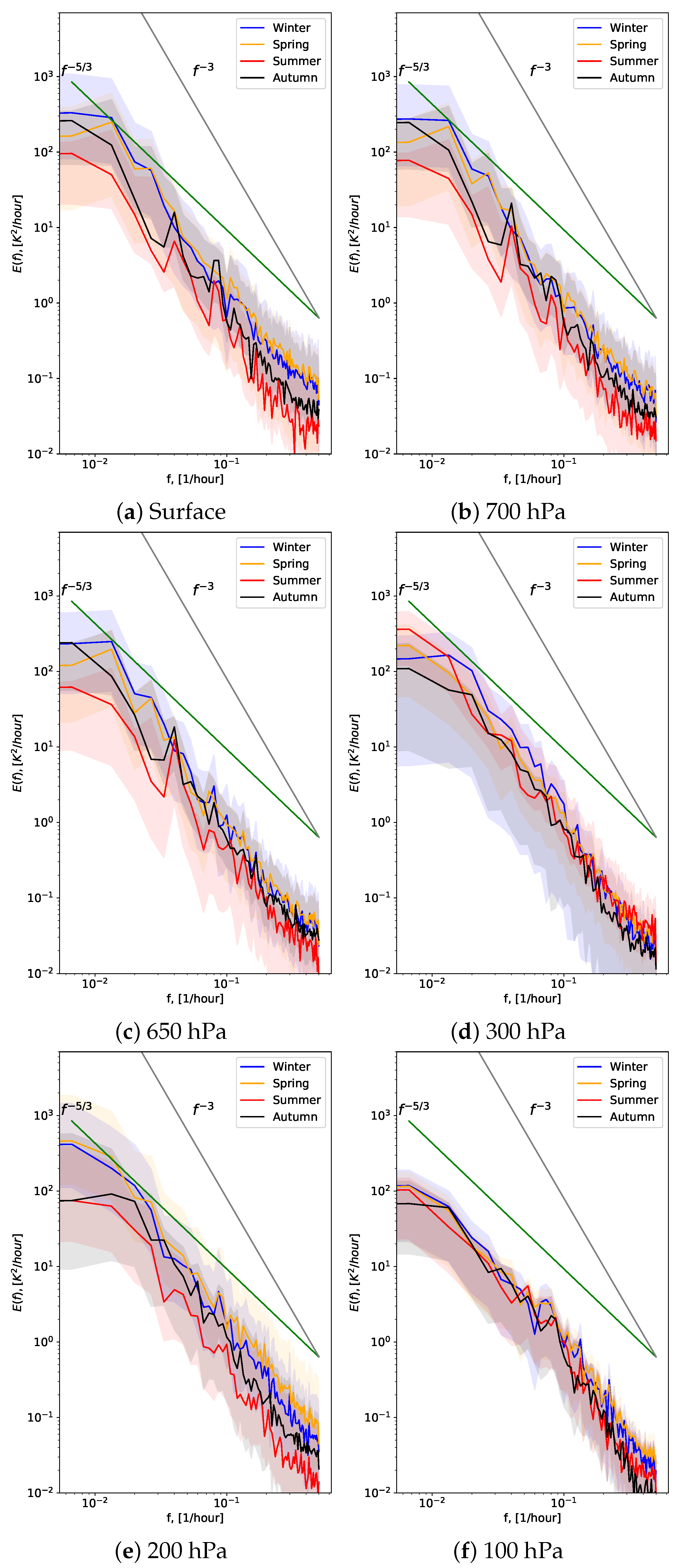
The energy spectra of both wind speed fluctuations and air temperature fluctuations are significantly deformed in time and space. Nevertheless, the data of experimental studies show that there is a dependence of the power spectral density on the frequency (period) of fluctuations in the spectra [21]. Each spectrum has two different regions with distinct slopes:

(i)

The region associated with enstrophy flux. In this region, the power spectral densities of wind speed fluctuations $E_V\left(f\right)$ as well as air temperature fluctuations $E\left(f\right)$ are proportional to frequency $f^{-3}$.

(ii)

The region associated with energy cascade. In this region, the power spectral densities $E_V\left(f\right)$ and $E\left(f\right)$ are proportional to frequency $f^{-5/3}$.

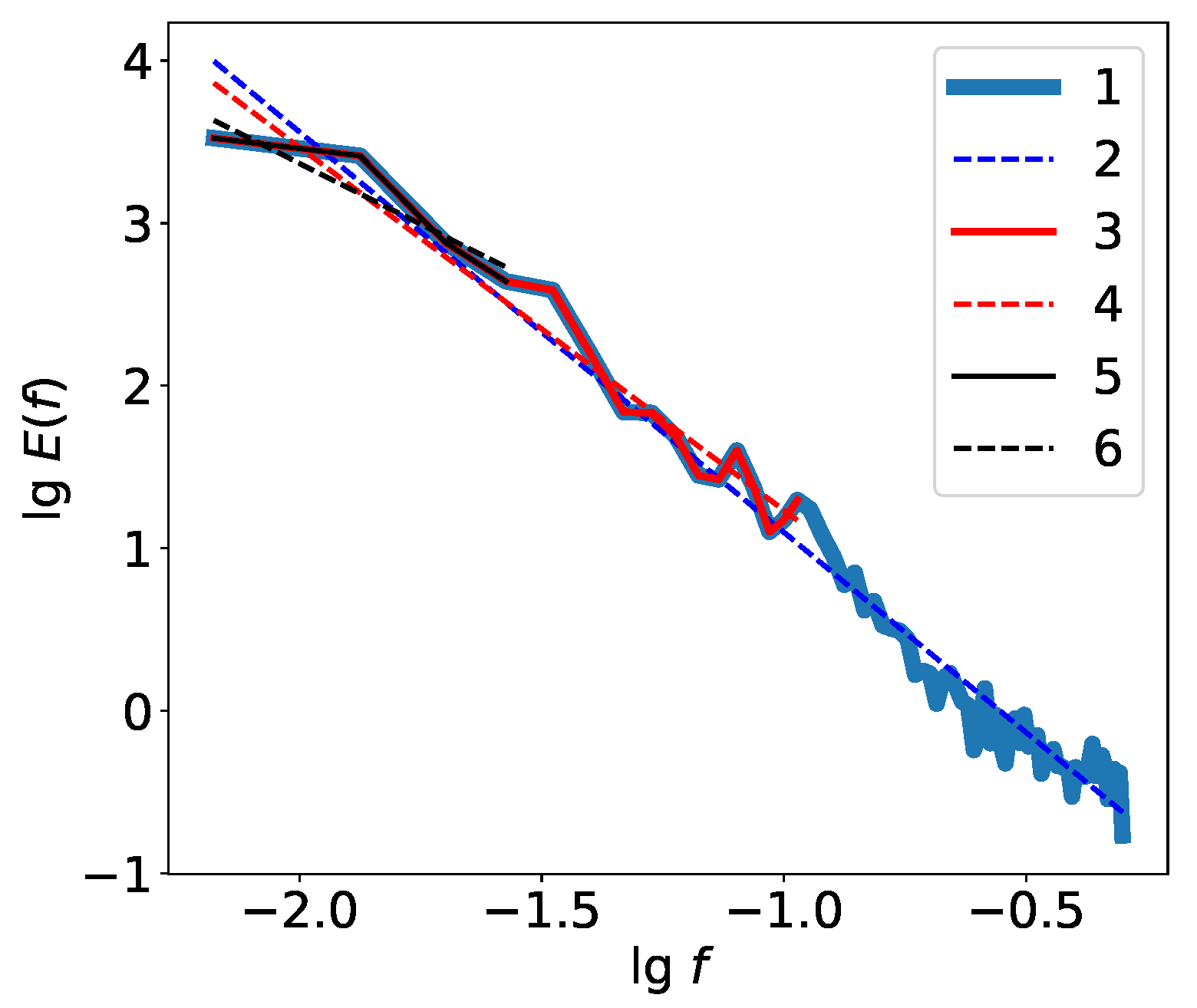
We suppose that, on average, atmospheric baroclinic disturbances determine the energy of small-scale turbulence at a given height (in combination with local factors). Thus, it can be assumed that the averaged energy spectrum can be approximated by two slopes in free atmosphere:

(i)

−3 in the low-frequency range, for scales $l>600$ km;

(ii)

−5/3 for mesoscales and micrometeorological range $l<600$ km;

(iii)

The turbulence spectrum is deformed in the atmospheric boundary layer.

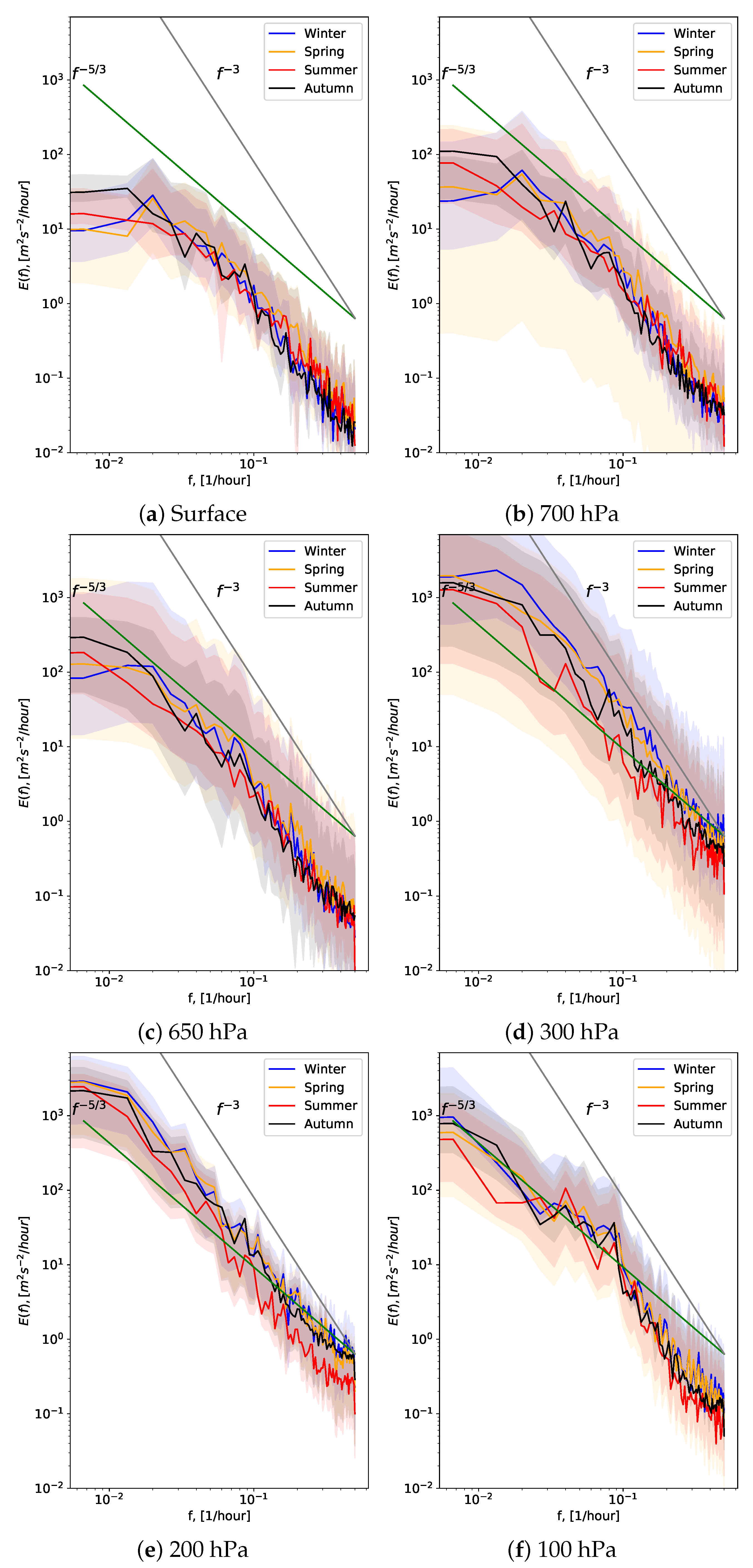
The spectrum of wind speed fluctuations in the atmospheric boundary layer contains a spectral plateau associated with the growth of small-scale turbulence energy. The paper [22] shows that the spectral plateau is observed under a neutral atmosphere as well as in convective conditions. In a stably stratified atmosphere, the plateau collapses on the low-frequency side of the micrometeorological range. In this case, the contribution of large-scale components of turbulence and mesoscale disturbances as well as wave interactions with respect to small-scale turbulence energy increases. Large-scale coherent components of the turbulence may be responsible for mixing across the entire flow thickness [23] and can induce changes in the energy structure of turbulent motions of smaller scales [24]. A feature of this spectral range is its transitional character from a mesoscale “gap” to an inertial interval. Moreover, a so-called buoyancy subrange is often distinguished in the spectrum. Atmospheric stratification and gravitational waves play an important role in this subrange [25,26]. The potential significance of the modulation effects of mesoscale fluctuations on turbulence was also pointed out in the study [27].

Significant results concerning the spectra were obtained by Larsen X.G. [28]. An analysis of changes in the averaged wind speed and its fluctuations made it possible to estimate the deformations of the full-scale spectrum with height. It is important that a positive slope in the low-frequency region of the micrometeorological interval (which we associate with the collapse of the spectral plateau) is observed in the surface layer of the atmosphere. The energy spectra corresponding to heights of 1.5–10 m demonstrate dependency $E_V\left(f\right)\sim f^1$ in the transition subrange [29]. At a height of 80 m, the plateau is practically not deformed. The slope of the spectrum becomes negative at higher levels.

It is worth nothing that the frequency dependencies of the power spectral density vary [30]. The energy in the large scale peak associated with baroclinic instability increases with height. At the same time, the energy of the small scale turbulence decreases. The spectra with the full range of atmospheric fluctuations at the Høvsøre site (Bøvlingbjerg, Denmark) confirm such changes in fluctuations with height in this transition subrange [31]. We believe that the energy of the small-scale turbulence is determined by the energy of baroclinic instability as well as the action of local factors at a given height (convective instability, mesoscale coherent structures and local vertical gradients of wind speed).

3. Turbulence Spectra in Uzbekistan

3.1. Methodology

There is no universal method for estimating $C_n^2$ at different heights in the atmosphere. This is mainly due to the physical features in the generation of turbulence in the atmospheric boundary layer and the free atmosphere. Moreover, the Kolmogorov model of homogeneous and isotropic turbulence is valid only for a narrow subrange of scales. In study [32], a global free atmosphere $\beta$ map has been obtained. In our opinion, the values of $\beta$ are significantly underestimated in the equatorial zone. We believe that the method for calculating optical turbulence characteristics, including $C_n^2$, must be selected and adapted for a given site. In study [17], $C_n^2\left(z\right)$ is given by Formula (4):

$$C_n^2\left(z\right)={\left(\frac{AP\left(z\right)}{T{\left(z\right)}^2}\right)}^2{\sigma }^2(f_L,z)\varphi (f,z),$$

(4)

where ${\sigma }^2(f_L,z)$ is the specific energy of the low frequency air temperature fluctuations, and $\varphi (f,z)$ is the function that takes into account the changes in the power spectral density in a wide ranges of scales. The function $\varphi (f,z)$ is a complex dependency of the power spectral density on frequency. In a simple case, $\varphi (f,z)$ may be calculated by using the following formula:

$$\varphi (f,z)=b_{mes}\frac{exp\left(\left(ln\frac{f_t}{f_L}\right){\gamma }_1+\left(ln\frac{f_l}{f_t}\right){\gamma }_2\right)}{0.125f_L}{f}_l^{5/3},$$

(5)

where ${\gamma }_1$ is the slope in the low frequency range, and ${\gamma }_1$ is the slope in the high frequency range. $f_L$ and $f_l$ are the frequencies in the low frequency range and high frequency interval, respectively. $f_t$ is the transition frequency between slopes. Coefficient $b_{mes}$ is calculated by comparing ${\int }_0^H{C}_n^2\left(z\right)dz$ estimated from the energy spectra and ${\int }_0^H{C}_n^2\left(z\right)dz$ calculated from optical observations of the image quality spoiled in the turbulent atmosphere [33]. On average, in the free atmosphere, it is possible to assume that $\varphi (f,z)$ at a given height is a constant at a given site (if ${\gamma }_1$= −3, ${\gamma }_2$ = −5/3).

In order to determine the possibilities of the method and to choose the optimal approach to calculate $C_n^2\left(z\right)$, we obtained the averaged energy spectra of fluctuations in the wind speed and air temperature at different levels in the atmosphere. In order to calculate the energy spectra, we used Era-5 reanalysis hourly data on pressure levels. The Era-5 database is the fifth-generation global atmospheric reanalysis with increased temporal (1 h), horizontal (0.25${}^{\circ }$) and vertical resolutions (137 model levels from the surface to 0.01 hPa) [34]. The sampling frequency of the data is one hour. The frequency spectra of the wind speed and air temperature were estimated with Fast Fourier Transform (FFT). Previously, we divided the initial dataset into 188 time series of 140 h duration. Then, we removed the linear trends in each time series. After calculating the spectra, we averaged spectra for both the air temperature fluctuations and wind speed fluctuations. As a result, we calculated the energy spectra of the air temperature fluctuations as well as the wind speed fluctuations for all pressure levels available in Era-5 reanalysis. However, we discuss only some spectra: the lower, middle and upper optically active atmosphere. The spectra were obtained in the surface layer of the atmosphere at the 700 hPa (350 m), 650 hPa (1 km), 300 hPa (6.5 km), 200 hPa (9.2 km) and 100 hPa (13.6 km).

3.2. Energy Spectra of the Air Temperature and Wind Speed Fluctuations at the Maidanak Observatory Site

Figure 1 and Figure 2 show the spectra of the air temperature as well as wind speed fluctuations at different pressure levels for all seasons at the Maidanak observatory site. At the Suffa observatory, the energy spectra of the air temperature and wind speed fluctuations are shown in Figure 3 and Figure 4, respectively. Each spectrum includes 95 % confidence interval.

Analysis of Figure 1 shows that the spectra in the surface layer have two distinct slopes. The spectra show a close to $f^{-5/3}$ power law in the high-frequency region and demonstrates, approximately, $f^{-3}$ power-law behavior in a narrow low-frequency region. The region with $f^{-5/3}$ power-law dependence narrows with height. This is confirmed by the increase in the total slopes calculated in a wide range (

Table 1. Spectral slopes at the Maidanak observatory site. Energy spectra of air temperature fluctuations.

Level, hPa	Season	${\mathit{s}}_1$	${\mathit{s}}_2$
Surface	Winter	−1.75	−2.13
	Spring	−1.80	−1.80
	Summer	−1.78	−2.17
	Autumn	−1.87	−2.18
700	Winter	−1.82	− 2.19
	Spring	−1.85	−1.85
	Summer	−1.76	−2.11
	Autumn	−1.87	−2.21
650	Winter	−1.92	−2.29
	Spring	−1.89	−1.89
	Summer	−1.92	−2.06
	Autumn	−1.86	−2.20
500	Winter	−2.05	−2.31
	Spring	−1.97	−1.87
	Summer	−1.83	−2.04
	Autumn	−1.89	−2.32
300	Winter	−2.45	−2.57
	Spring	−2.23	−2.23
	Summer	−1.84	−2.23
	Autumn	−2.21	−2.44
200	Winter	−2.32	−2.34
	Spring	−2.25	−2.25
	Summer	−2.21	−2.34
	Autumn	−2.11	−2.29
100	Winter	−2.52	−2.28
	Spring	−2.37	−2.37
	Summer	−2.28	−2.37
	Autumn	−2.87	−2.55
30	Winter	−2.96	−2.19
	Spring	−3.12	−3.13
	Summer	−3.14	−1.73
	Autumn	−3.32	−2.19

). In the higher layers, the spectra are close to ∼$f^{-3}$ dependency.

The spectra of wind speed fluctuations differ significantly from the spectra of air temperature fluctuations. In the lower layers of the atmosphere, the spectra possess a slope between −2.10 and −2.55 in a wide range of frequencies. A clear $f^{-3}$ power-law dependence in the low-frequency region was not distinguished in the surface layer. The energy of low-frequency fluctuations in wind speed increases with height. The range associated with $f^{-3}$ power-law dependence expands towards low frequencies. At the 100 hPa level, the spectra of wind speed fluctuations are similar to each other. The spectra of the air temperature fluctuations have a similar shape. However, the intensity of wind speed fluctuations increases in the range from 12 to 24 h.

By processing the time series of the air temperature, we calculated the energy in a low-frequency range from $f_1=6.7\times {10}^{-3}$ h${}^{-1}$ to $f_2=13.3\times {10}^{-3}$ h${}^{-1}$, as well as the energy in the high-frequency range from $f_3=0.36$ h${}^{-1}$ to $f_4=0.5$ h${}^{-1}$. These ranges correspond to high-frequency fluctuations and baroclinic atmospheric fluctuations. The energy values for each pressure level and season are provided in

Table 2. The mean values of energy ${\int }_{f_1}^{f_2}E\left(f\right)df$ and ${\int }_{f_3}^{f_4}{E}_l\left(f\right)df$ at the Maidanak observatory.

Level, hPa	Season	${\int }_{{\mathit{f}}_1}^{{\mathit{f}}_2}\mathit{E}\left(\mathit{f}\right)\mathit{df}$, ${{(}^{\mathit{o}})}^2$	${\int }_{{\mathit{f}}_3}^{{\mathit{f}}_4}{\mathit{E}}_{\mathit{l}}\left(\mathit{f}\right)\mathit{df}$, ${\left({}^{\mathit{o}}\right)}^2$
Surface	Winter	6.03	0.79
	Spring	4.43	0.96
	Summer	1.31	0.21
	Autumn	3.39	0.38
700	Winter	5.34	0.57
	Spring	3.81	0.65
	Summer	3.31	0.21
	Autumn	1.11	0.33
650	Winter	4.87	0.42
	Spring	3.43	0.47
	Summer	0.90	0.21
	Autumn	2.76	0.31
500	Winter	4.05	0.41
	Spring	2.61	0.40
	Summer	0.68	0.18
	Autumn	2.17	0.32
300	Winter	3.18	0.25
	Spring	2.75	0.30
	Summer	4.50	0.38
	Autumn	1.50	0.19
200	Winter	5.45	0.51
	Spring	6.89	0.87
	Summer	1.34	0.15
	Autumn	1.72	0.33
100	Winter	1.62	0.24
	Spring	1.51	0.32
	Summer	1.14	0.17
	Autumn	1.26	0.09
30	Winter	1.45	0.38
	Spring	0.37	0.24
	Summer	1.13	0.22
	Autumn	1.32	0.20

.

Strong air temperature fluctuations in both low-frequency and high-frequency ranges were observed in the lower atmosphere, which predominantly contributes to optical turbulence and the quality of astronomical images. At a pressure level of 200 hPa, relating to the height of the jet stream, air temperature fluctuations were also significant. It can be noted that the lowest intensity of air temperature fluctuations corresponds to the summer and autumn seasons. In winter and spring season, the intensity of the air temperature fluctuations increases. It is worth noting that the quality of astronomical images ($\beta$) at the Maidanak observatory changes in a similar manner. The image quality related to low values of $C_n^2$ is best in the summer and autumn [35].

3.3. Slopes in the Energy Spectra of the Atmospheric Turbulence at the Maidanak Observatory Site

In order to determine the slopes in the energy spectra of the atmospheric turbulence, we used an approach similar to that described in [36]. We used 73 spectral bands to determine the total slope. Our approach is based on linear regression. In order to determine the slopes, we used spectral ranges limited by different frequencies. An outline of the procedure is shown in Figure 5 and Figure 6. We estimated the slopes for the full-scale spectrum as well as in the narrower spectral ranges. At each step, we removed one band from the spectrum and calculated the spectral slope. First, we removed low frequency bands and considered the spectrum in the range from $T_{min}=2$ h to $T_{max}-mi$ ($T_{max}$ is the maximal period, m is the band width and i is a number of the shift) (Figure 5). Thus, we calculated slopes $s_1$ in the range limited by the low-frequency part.

Then, we removed high frequency bands and calculated spectral slopes $s_2$ in the range from $T_{max}$ to $T_{min}+mi$. Figure 6 shows an outline of the procedure used to determinate the slopes by removing the high-frequency bands. This approach, related to the determination of the slopes in limited spectral ranges, renders it possible to determine spectral ranges accurately. A range is inferred when the two criteria below are satisfied:

(i)

$s=<s>\pm \delta s$;

(ii)

$\delta s\le 0.1<s>$, where $<s>$ is an averaged slope, and $\delta s$ are fluctuations of the slope. Spectral slopes at the Maidanak observatory site are shown in

Table 3. Spectral slopes at the Maidanak observatory site. Energy spectra of wind speed fluctuations.

Level, hPa	Season	${\mathit{s}}_1$	${\mathit{s}}_2$
Surface	Winter	−2.55	−2.42
	Spring	−2.41	−2.41
	Summer	−2.30	−2.10
	Autumn	−2.45	−2.29
700	Winter	−2.32	− 2.42
	Spring	−2.26	−2.26
	Summer	−2.34	−2.15
	Autumn	−2.52	−2.43
650	Winter	−2.38	−2.34
	Spring	−2.32	−2.32
	Summer	−2.53	−2.23
	Autumn	−2.48	−2.47
500	Winter	−2.53	−2.29
	Spring	−2.47	−2.47
	Summer	−2.57	−2.31
	Autumn	−2.19	−2.38
300	Winter	−2.34	−2.42
	Spring	−2.67	−2.67
	Summer	−2.35	−2.42
	Autumn	−2.17	−2.37
200	Winter	−2.21	−2.48
	Spring	−2.48	−2.48
	Summer	−2.00	−2.32
	Autumn	−1.91	−2.20
100	Winter	−2.84	−2.53
	Spring	−2.80	−2.76
	Summer	−2.64	−2.54
	Autumn	−2.55	−2.47
30	Winter	−2.78	−2.39
	Spring	−3.07	−3.07
	Summer	−3.22	−2.04
	Autumn	−3.25	−2.42

. Figure 7 shows examples of the dependencies of the slopes on a number of removed bands $N_F$ in the spectra of the air temperature fluctuations at the observatories of Maidanak and Suffa in both the lower and upper layers of the atmosphere.

Figure 8 shows examples of dependencies of the slopes on a number of removed bands $N_F$ in the spectra of wind speed fluctuations at the Maidanak and Suffa observatories in both the lower and upper layers of the atmosphere. The shape of the red line indicates that there is a wide range with a slope between $-3$ and $-2$ at the Maidanak and Suffa observatories. The perturbations in the high frequency part of the spectra are most pronounced for the wind speed in the lower layers (line 1). Thus, we obtained the dependencies of the slopes on a number of removed bands $N_F$ and estimated the slope for a given spectral range. Further, the data were used in calculations of $C_n^2\left(z\right)$.

3.4. Energy Spectra of the Air Temperature and the Wind Speed Fluctuations at the Suffa Observatory Site

The astronomical observatory of Suffa is located on a high-mountain plateau in the spurs of the Turkestan ridge in the Republic of Uzbekistan. The height above the sea level of the Suffa observatory is close to the Maidanak observatory and equal to 2324 m.

The energy spectra of temperature fluctuations at the site of the Suffa observatory were similar to the spectra observed at the Maidanak Astronomical Observatory site. Figure 3 and Figure 4 show examples of energy spectra in the lower, middle and upper optically active atmosphere. It should be noted that the spectra are not as well approximated by the −5/3 power-law dependence in the high-frequency region (for mesoscales) in comparison with those of the Maidanak observatory. Taken in its entirety, at the sites of the observatories the spectra in the mesoscale range have slopes slightly steeper than −5/3. Table 2 and

Table 4. The mean values of energy ${\int }_{f_1}^{f_2}E\left(f\right)df$ and ${\int }_{f_3}^{f_4}{E}_l\left(f\right)df$ at the Suffa observatory.

Level, hPa	Season	${\int }_{{\mathit{f}}_1}^{{\mathit{f}}_2}\mathit{E}\left(\mathit{f}\right)\mathit{df}$, ${{(}^{\mathit{o}})}^2$	${\int }_{{\mathit{f}}_3}^{{\mathit{f}}_4}{\mathit{E}}_{\mathit{l}}\left(\mathit{f}\right)\mathit{df}$, ${{(}^{\mathit{o}})}^2$
Surface	Winter	5.16	0.87
	Spring	4.20	1.12
	Summer	1.40	0.33
	Autumn	3.47	0.50
700	Winter	4.53	0.71
	Spring	3.56	0.79
	Summer	1.21	0.28
	Autumn	2.94	0.35
650	Winter	4.14	0.60
	Spring	3.02	0.56
	Summer	0.95	0.23
	Autumn	2.59	0. 30
500	Winter	3.67	0.40
	Spring	2.55	0.38
	Summer	0.69	0.23
	Autumn	2.06	0.45
300	Winter	2.34	0.36
	Spring	2.42	0.35
	Summer	3.02	0.39
	Autumn	1.48	0.16
200	Winter	5.38	0.57
	Spring	6.65	0.93
	Summer	1.46	0.27
	Autumn	2.54	0.45
100	Winter	1.33	0.20
	Spring	1.27	0.31
	Summer	0.98	0.17
	Autumn	1.16	0.11
30	Winter	1.52	0.30
	Spring	0.40	0.22
	Summer	0.13	0.19
	Autumn	0.32	0.23

show that low-frequency temperature fluctuations are higher at the Maidanak observatory during the winter. In the summer, the baroclinicity of the atmosphere is significantly weakened, and its contribution to small-scale turbulence decreases at both the observatories. Spectral slopes at the Suffa observatory site are shown in

Table 5. Spectral slopes at the Suffa observatory site. Energy spectra of wind speed fluctuations.

Level, hPa	Season	${\mathit{s}}_1$	${\mathit{s}}_2$
Surface	Winter	−2.38	−2.06
	Spring	−2.61	−2.61
	Summer	−2.39	−1.89
	Autumn	−2.39	−2.21
700	Winter	−2.58	− 2.25
	Spring	−2.53	−2.53
	Summer	−2.37	−2.03
	Autumn	−2.16	−2.27
650	Winter	−2.70	−2.12
	Spring	−2.59	−1.85
	Summer	−2.42	−2.03
	Autumn	−2.14	−2.20
500	Winter	−2.07	−2.29
	Spring	−1.95	−1.95
	Summer	−1.71	−1.99
	Autumn	−1.77	−2.06
300	Winter	−2.18	−2.37
	Spring	−2.15	−2.15
	Summer	−1.72	−2.15
	Autumn	−2.27	−2.46
200	Winter	−2.24	−2.29
	Spring	−2.21	−2.21
	Summer	−2.07	−2.21
	Autumn	−2.06	−2.25
100	Winter	−2.67	−2.35
	Spring	−2.35	−2.35
	Summer	−2.43	−2.34
	Autumn	−2.75	−2.44
30	Winter	−3.10	−2.25
	Spring	−3.26	−3.26
	Summer	−3.23	−1.72
	Autumn	−3.23	−2.13

and

Table 6. Spectral slopes at the Suffa observatory site. Energy spectra of air temperature fluctuations.

Level, hPa	Season	${\mathit{s}}_1$	${\mathit{s}}_2$
Surface	Winter	−1.69	−2.08
	Spring	−1.73	−1.73
	Summer	−2.00	−2.07
	Autumn	−1.89	−2.21
700	Winter	−1.73	− 2.11
	Spring	−1.82	−1.82
	Summer	−1.95	−2.06
	Autumn	−1.77	−2.21
650	Winter	−1.71	−2.29
	Spring	−1.85	−1.89
	Summer	−1.89	−2.06
	Autumn	−1.77	−2.20
500	Winter	−2.05	−2.31
	Spring	−1.97	−1.87
	Summer	−1.83	−2.04
	Autumn	−1.89	−2.32
300	Winter	−2.45	−2.57
	Spring	−2.23	−2.23
	Summer	−1.84	−2.23
	Autumn	−2.21	−2.44
200	Winter	−2.32	−2.34
	Spring	−2.25	−2.25
	Summer	−2.21	−2.34
	Autumn	−2.11	−2.29
100	Winter	−2.52	−2.28
	Spring	−2.37	−2.37
	Summer	−2.28	−2.37
	Autumn	−2.87	−2.55
30	Winter	−2.96	−2.19
	Spring	−3.12	−3.13
	Summer	−3.14	−1.73
	Autumn	−3.32	−2.19

. The energy spectra of the wind speed fluctuations have slope ranges from −3.25 to −1.91. In the surface layer of the atmosphere, the range with −5/3 power-law dependence is not observed. At the Suffa site, the −3 power-law dependence corresponds to a narrow range from 2 to 5.9 h at 700 hPa level. Indirectly, this may indicate that the image quality for the Maidanak observatory is higher than that of the Suffa observatory.

Thus, the spectra do not demonstrate a clear −3 slope in a wide range of scales. In order to determine the range with the −3 slope, we used the following approach. We selected a subrange containing three bands and estimated the slopes in different spectral subranges (from left to right in the spectrum). Then, we estimated the slopes for 3$+mi$ spectral bands. An outline of the procedure used to determinate the slopes with different sizes of bands is shown in Figure 9. Changes in widths of the subranges make it possible to reveal a −3 slope. Some results for the atmospheric boundary layer and the free atmosphere are given in the

Table 7. Spectral slopes at Maidanak and Suffa observatories.

		Suffa Observatory				Maidanak Observatory
Level, hPa	Season	Slope	ft1, 1/h	ft2, 1/h/	Slope	ft1, 1/h	ft2, 1/h
Air temperature
Surface	Winter	−2.98	13.3 $\times {10}^{-3}$	4.80 $\times {10}^{-2}$	−3.03	13.3 $\times {10}^{-3}$	3.33 $\times {10}^{-2}$
	Spring	−3.00	13.3 $\times {10}^{-3}$	2.10 $\times {10}^{-2}$	−3.00	13.3 $\times {10}^{-3}$	2.30 $\times {10}^{-2}$
	Summer	−2.99	13.3 $\times {10}^{-3}$	3.83 $\times {10}^{-2}$	−2.96	13.3 $\times {10}^{-3}$	3.00 $\times {10}^{-2}$
	Autumn	−3.00	13.3 $\times {10}^{-3}$	2.99 $\times {10}^{-2}$	−2.93	13.3 $\times {10}^{-3}$	3.33 $\times {10}^{-2}$
200	Winter	−2.93	20.0 $\times {10}^{-3}$	4.67 $\times {10}^{-2}$	−3.02	26.6 $\times {10}^{-3}$	4.00 $\times {10}^{-2}$
	Spring	−3.00	13.3 $\times {10}^{-3}$	2.08 $\times {10}^{-2}$	−3.02	26.6 $\times {10}^{-3}$	4.00 $\times {10}^{-2}$
	Summer	−2.89	20.0 $\times {10}^{-3}$	3.80 $\times {10}^{-2}$	−3.00	20.0 $\times {10}^{-3}$	4.00 $\times {10}^{-2}$
	Autumn	−3.00	20.0 $\times {10}^{-3}$	2.99 $\times {10}^{-2}$	−3.10	20.0 $\times {10}^{-3}$	3.33 $\times {10}^{-2}$
Wind speed
Surface	Winter	−2.96	10.70 $\times {10}^{-2}$	24.70 $\times {10}^{-2}$	−3.03	10.0 $\times {10}^{-2}$	3.00 $\times {10}^{-2}$
	Spring	−3.03	14.60 $\times {10}^{-2}$	24.00 $\times {10}^{-2}$	−3.00	10.0 $\times {10}^{-2}$	2.60 $\times {10}^{-2}$
	Summer	−2.95	12.70 $\times {10}^{-2}$	24.00 $\times {10}^{-2}$	−2.96	10.0 $\times {10}^{-2}$	4.00 $\times {10}^{-2}$
	Autumn	−2.96	9.33 $\times {10}^{-2}$	24.70 $\times {10}^{-2}$	−2.93	10.0 $\times {10}^{-2}$	4.00 $\times {10}^{-2}$
200	Winter	−2.90	10.0 $\times {10}^{-1}$	18.67 $\times {10}^{-2}$	−3.00	10.0 $\times {10}^{-2}$	3.20 $\times {10}^{-2}$
	Spring	−2.99	10.00 $\times {10}^{-2}$	16.00 $\times {10}^{-2}$	−2.99	10.00 $\times {10}^{-2}$	3.00 $\times {10}^{-2}$
	Summer	−2.89	20.00 $\times {10}^{-3}$	3.80 $\times {10}^{-2}$	−2.90	10.00 $\times {10}^{-2}$	4.00 $\times {10}^{-2}$
	Autumn	−2.98	12.00 $\times {10}^{-3}$	21.33 $\times {10}^{-2}$	−3.00	10.00 $\times {10}^{-2}$	3.33 $\times {10}^{-2}$

. An analysis of the slopes shows spectra containing narrow subranges with −3 slope.

4. Conclusions

In this paper, we discuss features of the energy spectra of meteorological parameter fluctuations by processing and analysing the data of modern Era-5 reanalysis at the sites of Maidanak and Suffa observatories. Below, we summarise key points about the energy spectra.

(i)

The energy spectra of air temperature fluctuations at the Maidanak and Suffa observatories, calculated from the Era-5 reanalysis data, approximately obey power-law dependencies −5/3 in a narrow high-frequency range and have slope ranges from −3 to −2 in the low-frequency range. A clear −3 dependency was observed only for a narrow spectral interval.

(ii)

The spectra of wind speed fluctuations in the upper atmosphere (at levels from 200 to 100 hPa) were similar to each other. The energy of the high-level wind speed spectra varies within narrow limits at the Maidanak and Suffa observatories.

(iii)

The energy spectra of the wind speed fluctuations differ significantly from the spectra of the air temperature fluctuations. In the low-frequency range, a narrow range with −3 power-law dependence was observed. The existence of a range of scales with power-law dependence −3 indicates a developed enstropy transfer. In the near-surface atmospheric layer, the slopes changed significantly. The spectra in the low-frequency range degenerated, namely, low-frequency fluctuations of the wind speed were suppressed. It is possible that the suppression of the low-frequency wind speed fluctuations is one of the reasons for the growth of the energy of micrometeorological turbulence in the surface layer.

(iv)

At the site of the Suffa observatory, the −3 power-law dependence corresponds to a range from 2 to 5.9 h at 700 hPa level (there is no −5/3 pronounced slope at the Maidanak observatory). This may indicate that the image quality at the Maidanak observatory is higher than that of the Suffa observatory.

(v)

Compared to the classical spectra, one may observe often a steeper slope than −5/3 in the mesoscale range at the Maidanak and Suffa observatories.

(vi)

The specific energy of baroclinic instability at the Maidanak and Suffa observatories is high during the year at pressure levels ($P>100$ hPa). Taking into account that baroclinic instability is associated with large vertical gradients of the wind speed, we can recommend the method outlined in [17] to calculate $C_n^2\left(z\right)$ at the Maidanak and Suffa observatories.

(vii)

At the Maidanak observatory, the character of seasonal changes in low-frequency and high-frequency temperature fluctuations associated with baroclinic instability of the atmosphere was qualitatively in good agreement with the changes observed in [35]. The best atmospheric conditions determined by the energy of the temperature spectra are also observed in the summer and autumn seasons.

It should be noted that this paper presents the first results of studies of baroclinic instability by using the Era-5 dataset with higher spatial and temporal resolutions. The results obtained will be further used to determine and analyze the height profiles of optical turbulence over astronomical observatories located in different latitudinal zones. Furthermore, in order to calculate $C_n^2\left(z\right)$, we plan to use sensors measuring meteorological parameters in the surface layer of the atmosphere as well as the data of DIMM measurements of image motion [37,38,39,40].

References

1. Hidalgo, S.L.; Muñoz-Tuñón, C.; Castro-Almazán, J.A.; Varela, A.M. Canarian Observatories Meteorology; Comparison of OT and ORM using Regional Climate Reanalysis. Publ. Astron. Soc. Pac. 2021, 133, 105002. [Google Scholar] [CrossRef]
2. Hellemeier, J.A.; Yang, R.; Sarazin, M.; Hickson, P. Weather at selected astronomical sites—An overview of five atmospheric parameters. Mon. Not. R. Astron. Soc. 2019, 482, 4941–4950. [Google Scholar] [CrossRef]
3. Otarola, A.; De Breuck, C.; Travouillon, T.; Matsushita, S.; Nyman, L.-A.; Wootten, A.; Radford, S.J.E.; Sarazin, M.; Kerber, F.; Pérez-Beaupuits, J.P. Precipitable Water Vapor, Temperature, and Wind Statistics at Sites Suitable for mm and Submm Wavelength Astronomy in Northern Chile. Publ. Astron. Soc. Pac. 2019, 131, 045001. [Google Scholar] [CrossRef]
4. Bubnov, G.M.; Artemenko, Y.N.; Vdovin, V.F.; Danilevsky, D.B.; Zinchenko, I.I.; Nosov, V.I.; Nikiforov, P.L.; Shanin, G.I.; Raupov, D.A. The Results of Astroclimate Observations in the Short-Wave Length Interval of the Millimeter-Wave Range on the Suffa Plateau. Radiophys. Quantum Electron. 2017, 59, 763–771. [Google Scholar] [CrossRef]
5. Lotfy, E.R.; Abbas, A.A.; Zaki, S.A.; Harun, Z. Characteristics of Turbulent Coherent Structures in Atmospheric Flow under Different Shear–Buoyancy Conditions. Bound.-Layer Meteorol. 2019, 173, 115–141. [Google Scholar] [CrossRef]
6. Adrian, R.J.; Meinhart, C.D.; Tomkins, C.D. Vortex organization in the outer region of the turbulent boundary layer. J. Fluid Mech. 2000, 422, 1–54. [Google Scholar] [CrossRef] [Green Version]
7. Kovadlo, P.G.; Shikhovtsev, A.Y. The study of turbulence and optical instability in stably stratified Earth’s atmosphere. Proc. SPIE 2015, 9680, 968074. [Google Scholar] [CrossRef]
8. Fritts, D.C.; Wang, L.; Geller, M.A.; Lawrence, D.A.; Werne, J.; Balsley, B.B. Numerical modeling of multiscale dynamics at high Reynodls numbers: Instabilities, turbulence, and an assessment of Ozmidov and Thorpe scales. J. Atmos. Sci. 2016, 74, 555–578. [Google Scholar] [CrossRef]
9. Tung, K.K.; Orlando, W.W. The k−3 and k−5/3 Energy Spectrum of Atmospheric Turbulence: Quasigeostrophic Two-Level Model Simulation. J. Atmos. Sci. 2003, 60, 824–835. [Google Scholar] [CrossRef] [Green Version]
10. Fiorino, S.; Bose-Pillai, S.; Keefer, K. Re-Visiting Acoustic Sounding to Advance the Measurement of Optical Turbulence. Appl. Sci. 2021, 11, 7658. [Google Scholar] [CrossRef]
11. Osborn, J.; Wilson, R.; Butterley, T.; Shephard, H.; Sarazin, M. Profiling the surface layer of optical turbulence with SLODAR. Mon. Not. R. Astron. Soc. 2010, 406, 1405–1408. [Google Scholar] [CrossRef]
12. Wang, Z.; Zhang, L.; Kong, L.; Bao, H.; Guo, Y.; Rao, X.; Zhong, L.; Zhu, L.; Rao, C. A modified S-DIMM+: Applying additional height grids for characterizing daytime seeing profiles. Mon. Not. R. Astron. Soc. 2018, 478, 1459–1467. [Google Scholar] [CrossRef]
13. Zhong, L.; Zhang, L.; Shi, Z.; Tian, Y.; Guo, Y.; Kong, L.; Rao, X.; Bao, H.; Zhu, L.; Rao, C. Wide field-of-view, high-resolution Solar observation in combination with ground layer adaptive optics and speckle imaging. Astron. Astrophys. 2020, 637, A99. [Google Scholar] [CrossRef]
14. Xu, M.; Shao, S.; Liu, Q.; Sun, G.; Han, Y.; Weng, N. Optical Turbulence Profile Forecasting and Verification in the Offshore Atmospheric Boundary Layer. Appl. Sci. 2021, 11, 8523. [Google Scholar] [CrossRef]
15. Han, Y.; Yang, Q.; Liu, N.; Zhang, K.; Qing, C.; Li, X.; Wu, X.; Luo, T. Analysis of wind-speed profiles and optical turbulence above Gaomeigu and the Tibetan Plateau using ERA5 data. Mon. Not. R. Astron. Soc. 2021, 501, 4692–4701. [Google Scholar] [CrossRef]
16. Cai, J.; Li, X.; Zhan, G.; Wu, P.; Xu, C.; Qing, C.; Wu, X. A new model for the profiles of optical turbulence outer scale and Cn2 on the coast. Acta Phys. Sin. 2018, 67, 014206. [Google Scholar] [CrossRef]
17. Kovadlo, P.G.; Lukin, V.P.; Shikhovtsev, A.Y. Development of the Model of Turbulent Atmosphere at the Large Solar Vacuum Telescope Site as Applied to Image Adaptation. Atmos. Ocean. Opt. 2019, 32, 202–206. [Google Scholar] [CrossRef]
18. Shikhovtsev, A.; Kovadlo, P.; Lukin, V. Temporal Variations of the Turbulence Profiles at the Sayan Solar Observatory Site. Atmosphere 2019, 10, 499. [Google Scholar] [CrossRef] [Green Version]
19. Bolbasova, L.A.; Shikhovtsev, A.Y.; Kopylov, E.A.; Selin, A.A.; Lukin, V.P.; Kovadlo, P.G. Daytime optical turbulence and wind speed distributions at the Baikal Astrophysical Observatory. Mon. Not. R. Astron. Soc. 2019, 482, 2619–2626. [Google Scholar] [CrossRef]
20. Shikhovtsev, A.Y.; Kiselev, A.V.; Kovadlo, P.G.; Kolobov, D.Y.; Lukin, V.P.; Tomin, V.E. Method for Estimating the Altitudes of Atmospheric Layers with Strong Turbulence. Atmos. Ocean. Opt. 2020, 33, 295–301. [Google Scholar] [CrossRef]
21. Nastrom, G.D.; Gage, K.S. A Climatology of Atmospheric Wavenumber Spectra of Wind and Temperature Observed by Commercial Aircraft. J. Atmos. Sci. 1985, 42, 950–960. [Google Scholar] [CrossRef] [Green Version]
22. Cheynet, E.; Jakobsen, J.B.; Reuder, J. Velocity Spectra and Coherence Estimates in the Marine Atmospheric Boundary Layer. Bound.-Layer Meteorol. 2018, 169, 429–460. [Google Scholar] [CrossRef]
23. Flores, O.; Riley, J.J. Analysis of Turbulence Collapse in the Stably Stratified Surface Layer Using Direct Numerical Simulation. Bound.-Layer Meteorol. 2011, 139, 241–259. [Google Scholar] [CrossRef]
24. Lukin, V.P.; Nosov, E.V.; Nosov, V.V.; Torgaev, A.V. Causes of non-Kolmogorov turbulence in the atmosphere. Appl. Opt. 2016, 55, B163–B168. [Google Scholar] [CrossRef] [PubMed]
25. Avsarkisov, V. On the Buoyancy Subrange in Stratified Turbulence. Atmosphere 2020, 11, 659. [Google Scholar] [CrossRef]
26. Cheng, Y.; Li, Q.; Argentini, S.; Sayde, C.; Gentine, P. A Model for Turbulence Spectra in the Equilibrium Range of the Stable Atmospheric Boundary Layer. J. Geophys. Res. Atmos. 2020, 125, e2019JD03219. [Google Scholar] [CrossRef]
27. Lotfy, E.R.; Zaki, S.A.; Harun, Z. Modulation of the atmospheric turbulence coherent structures by mesoscale motions. J. Braz. Soc. Mech. Sci. Eng. 2018, 40, 178. [Google Scholar] [CrossRef]
28. Larsén, X.G.; Larsen, S.E.; Petersen, E.L. Full-Scale Spectrum of Boundary-Layer Winds. Bound.-Layer Meteorol. 2016, 159, 349–371. [Google Scholar] [CrossRef] [Green Version]
29. Drobinski, P.; Carlotti, P.; Newsom, R.K.; Banta, R.M.; Foster, R.C.; Redelsperger, J.-L. The Structure of the Near-Neutral Atmospheric Surface Layer. J. Atmos. Sci. 2004, 61, 699–714. [Google Scholar] [CrossRef]
30. Wang, J.-X.; Yang, Q.-S.; Sun, L.; Li, B.; Liu, M. Analysis of the wind speed spectrum in the urban area of Beijing based on the measured data of the Ma Dian Qiao Bei meteorological tower in 2013. Gongcheng Lixue/Eng. Mech. 2020, 37, 250–256. [Google Scholar] [CrossRef]
31. Mikkelson, T.; Larsen, S.E.; Jørgensen, H.E.; Astrup, P.; Larsén, H.G. Scaling of turbulence spectra measured in strong shear flow near the Earth’s surface. Phys. Scr. 2017, 92, 124002. [Google Scholar] [CrossRef] [Green Version]
32. Osborn, J.; Sarazin, M. Atmospheric turbulence forecasting with a General Circulation Model for Cerro Paranal. Mon. Not. R. Astron. Soc. 2014, 480, 1278–1299. [Google Scholar] [CrossRef] [Green Version]
33. Bolbasova, L.A.; Shikhovtsev, A.Y.; Kovadlo, P.G.; Avdeev, F.A.; Lukin, V.P. Development of a model of atmospheric turbulence at Baikal Astrophysical Observatory site of the Large Solar Vacuum Telescope. Proc. SPIE 2018, 10833, 108331P. [Google Scholar] [CrossRef]
34. Hersbach, H.; Bell, B.; Berrisford, P.; Hirahara, S.; Horányi, A.; Muñoz-Sabater, J.; Nicolas, J.; Peubey, C.; Radu, R.; Schepers, D.; et al. The ERA5 global reanalysis. Q. J. R. Meteorol. Soc. 2020, 146, 1999–2049. [Google Scholar] [CrossRef]
35. Artamonov, B.P.; Bruevich, V.V.; Gusev, A.S.; Ezhkova, O.V.; Ibrahimov, M.A.; Ilyasov, S.P.; Potanin, S.A.; Tillaev, Y.A.; Ehgamberdiev, S.A. Seeing and Atmospheric Extinction at Mt. Maidanak Observatory from Observations with the 1.5-m AZT-22 Telescope. Astron. Rep. 2010, 54, 1019–1031. [Google Scholar] [CrossRef]
36. Luce, H.; Kantha, L.; Hashiguchi, H.; Lawrence, D. Estimation of Turbulence Parameters in the Lower Troposphere from ShUREX (2016–2017) UAV Data. Atmosphere 2019, 10, 384. [Google Scholar] [CrossRef] [Green Version]
37. Ehgamberdiev, S.A.; Baijumanov, A.K.; Ilyasov, S.P.; Sarazin, M.; Tillayev, Y.A.; Tokovinin, A.A.; Ziad, A. The astroclimate of Maidanak Observatory in Uzbekistan. Astron. Astrophys. Suppl. Ser. 2000, 145, 293–304. [Google Scholar] [CrossRef] [Green Version]
38. Ehgamberdiev, S.A. Modern astronomy at the Maidanak observatory in Uzbekistan. Nat. Astron. 2018, 2, 349–351. [Google Scholar] [CrossRef]
39. Kornilov, V.; Ilyasov, S.; Voziakova, O.; Tillaev, Y.; Safonov, B.; Ibragimov, M.; Shatsky, N.; Ehgamberdiev, S. Measurement of optical turbulence in free atmosphere above Mt.Maidanak in 2005–2007. Astron. Lett. 2009, 35, 547–554. [Google Scholar] [CrossRef] [Green Version]
40. Tillayev, Y.; Azimov, A.; Hafizov, A. Astronomical Seeing at Maidanak Observatory during the Year 2018. Galaxies 2021, 9, 38. [Google Scholar] [CrossRef]
Figure 1. Energy spectra of air temperature fluctuations at the Maidanak observatory site.
Atmosphere 12 01614 g001
Figure 2. Energy spectra of wind speed fluctuations at the Maidanak observatory site.
Atmosphere 12 01614 g002
Figure 3. Energy spectra of air temperature fluctuations at the Suffa observatory site.
Atmosphere 12 01614 g003
Figure 4. Energy spectra of wind speed fluctuations at the Suffa observatory site.
Atmosphere 12 01614 g004
Figure 5. Outline of the procedure used to determine the slopes with low-frequency bands removed. Line 1 corresponds to a full-scale spectrum. Lines 3 and 5 correspond to the regions of the spectra when we remove bands from the side of low frequencies. Lines 2, 4 and 6 correspond to the spectral slopes −2.46, −2.09, −2.47 respectively.
Atmosphere 12 01614 g005
Figure 6. Outline of the procedure used to determine the slopes with the high-frequency bands removed. Line 1 corresponds to a full-scale spectrum. Lines 3 and 5 correspond to the regions of the spectra when we remove bands from the side of high frequencies. Lines 2, 4 and 6 correspond to the spectral slopes −2.46, −2.23, −1.50 respectively.
Atmosphere 12 01614 g006
Figure 7. The dependencies of the slopes on N F at the observatories of Maidanak and Suffa. Spectra of air temperature fluctuations. Line 1 corresponds to the procedure when we remove bands from the side of low frequencies in the spectrum. Line 2 corresponds to the case when we remove bands from the side of high frequencies.
Atmosphere 12 01614 g007
Figure 8. The dependencies of the slopes on N F at the observatories of Maidanak and Suffa. The dependencies calculated from the spectra of the wind speed fluctuations. Line 1 corresponds to the procedure when we remove bands from the side of low frequencies in the spectrum. Line 2 corresponds to the case when we remove bands from the side of high frequencies.
Atmosphere 12 01614 g008
Figure 9. Outline of the procedure for determining the slopes with different sizes of spectral bands. Line 1 corresponds to a full-scale spectrum. Line 2 corresponds to a range from 6.0 to 9.4 h. Line 3 corresponds to a range from 10.7 to 37.5 h.
Atmosphere 12 01614 g009