Air Quality Assessment in the Central Mediterranean Sea (Tyrrhenian Sea): Anthropic Impact and Miscellaneous Natural Sources, including Volcanic Contribution, on the Budget of Volatile Organic Compounds (VOCs)

Abstract

The results of air pollution assessment during a 2017 cruise of the research ship “Minerva Uno” in the Tyrrhenian Sea are reported. Volatile Organic Compounds (VOCs), Oxygenated Volatile Organic Compounds (OVOCs), and pollutants such as nitrogen oxides, ozone, and sulphur dioxide were monitored throughout the cruise. The shallow waters at ten sites of the investigated area were also analyzed. Organic compounds such as n-alkanes showed a bimodal distribution with a maximum at C5–C6 and C10–C11 at sites the most affected by anthropic impact, whereas remote sites showed a unimodal distribution with maximum at C10–C11. The most abundant atmospheric OVOC was acetone (3.66 μg/m³), accounting for 38%; formaldehyde (1.23 μg/m³) and acetaldehyde (0.99 μg/m³) made up about 22–29% of the total. The influence of some natural sources as volcanoes, in the southern part of the Tyrrhenian Sea near the Aeolian arc was studied. This source did not induce any noticeable effect on the total amount of hydrocarbons nor on the levels of trace gases such as CFCs, whereas the trends of sulphur dioxide seemed to confirm a possible contribution. The impact of underwater emissions was observed near the Panarea and Vulcano islands, where lower pHs, high levels of Fe and Mn, and diagnostic of vent activity, were measured.

1. Introduction

Many anthropic and natural contributions, which presently have not been fully unfolded, constitute the blend of possible sources affecting the air quality in the Mediterranean Basin, due to local emissions and to long-range transport of pollution from other continents [1]. The anthropogenic pressure of the densely populated coasts bordering this enclosed sea, with large urban agglomeration [2], and different anthropic activities (e.g., industrial, manufacturing, energy production) and maritime transport facilities, is certainly the driving factor in determining the overall air quality of the area. As much as 20% of seaborne trade, 10% of world container traffic and over 200 million passengers pass through the Mediterranean basin every year (https://www.medqsr.org/maritime-transport accessed on 2 September 2021).

Emissions coming from several natural sources, such as vegetation, wildfires, and volcanic activity, should also be accounted for, and especially the last source since it can significantly impact the southeastern part of the Tyrrhenian Sea. In addition, the effect of these sources can be further intensified by peculiar climatic conditions favoring photochemical pollution, particularly in hot periods when the precipitation is scarce and the ventilation, mainly due to mild breezes, is poor [3]. All these factors make this area a climate change “hot spot” [4].

Atmospheric VOCs have both natural and anthropogenic sources [5,6]. They play a central role in the production of the tropospheric ozone (O₃) and secondary organic aerosol (SOA), together with nitrogen oxides (NO_x) and solar radiation, and influence the atmospheric chemistry, air quality, and climate processes.

In addition to local emissions, long-range transport can also give a significant contribution, in particular to oxygenated Volatile Organic Compounds (OVOCs) as shown by Derstroff [7] who carried out an extensive study as part of the Research Program CYPHEX (CYprus PHotochemical EXperiment 2014).

Research activity in the Mediterranean basin was also carried out by the Institute of Atmospheric Pollution Research of the National Research Council (CNR-IIA) in the framework of the Med-Oceanor measurement program through cruise campaigns performed regularly since 2000. In 2015 the cruise of the research ship “Minerva Uno” followed a route in the central Mediterranean area (Tyrrhenian Sea) which also included the Aeolian Islands [8,9] and in 2017 the evaluation of the impact of this geologically active field on air quality of the southeastern area of Tyrrhenian Sea represented one of the research objectives of the cruise [10].

The Aeolian volcanic arc is composed by seven islands and several seamounts. Both active aerial cones and submerged seeps are present in the area, at the Stromboli and Vulcano islands, but emissions in the form of submarine vents are widespread located in a larger area. Along its northeastern coast, at Levante Bay, Vulcano Island presents gas vents in correspondence of an active fault, at a rather low depth (less than 1 m) on the southwestern part of the bay [11]. The venting gas field extends over a wide area in the Isthmus zone.

The assessment of Volatile Organic Compounds (VOCs) and Oxygenated Volatile Organic Compounds (OVOCs) concentrations in air samples collected through discontinuous active sampling during the 2017 cruise on-board the research ship “Minerva Uno” is reported in this study, with the aim of characterizing and highlighting the chemically different sites encountered.

Volcanic emission contribution to the organic compounds budget in the atmosphere has been previously studied [12,13,14], as well as halogen plume chemistry [15,16,17] despite showing contradictory results. The studies conducted on Vulcano Island (Aeolian Archipelago) by Schwandner et al. [16,17] indicate that the presence of halocarbons in volcanic emissions are significant, whereas Frische et al. [18] concluded that the atmospheric contamination of volcanic gases should be accounted for, in order to avoid overestimation. In agreement with this study, Tassi et al. [19] report the CFCs concentration at the Solfatara crater (Phlegraean Fields), to be likely due to air contamination. Butler et al. [20] also excluded the contribution of natural sources to most CFCs present in the environment.

As stated by Mather et al. [21] the mechanisms through which these compounds are released by volcanic or hydrothermal systems are still not definitely understood. Different pathways are proposed: gas-phase radical reactions of light alkanes and thermal cracking of longer chain hydrocarbons to shorter chain free radicals, then reacting with halogens and on rock surfaces by magmatic hydrogen halides. Therefore, improving the knowledge of the composition of the air nearby volcanic sites or geothermal active fields and monitoring a wide range of different atmospheric VOCs, among which CFCs, could be of help at this regard.

Moreover, shallow seawater collection followed by the assessment of general parameters as pH, ionic species, and metals content could provide further information on the impact of spot geogenic sources on its composition. On the other hand, the determination of some organic species, such as carbonyls and acidic components as dicarboxylic acids (DCAs), in the seawater could enhance the knowledge on the photochemical degradation of dissolved organic matter [22,23], the microbial degradation of long-chain lipids [24], and also the diffusion from surface sediments (especially for oxalic acid) [25]. Since these compounds make up a reservoir of secondary organic aerosol (SOA), then transferred from marine surface waters to the atmosphere, their potential impact on the Earth’s radiative forcing and climate, due to the cloud condensation nuclei (CCN) activity [26,27,28] has not to be neglected. Studies on these compounds in surface seawaters are rare, especially in the Mediterranean Sea [25,29,30]. Therefore, this study was also intended to improve our understanding of the relative contributions of anthropogenic and marine sources to the atmospheric organic compounds budget.

In summary the scope of this study was to evaluate the impact of natural and anthropic sources in the Mediterranean area air quality by examining the concentration levels of several VOCs, both in the atmosphere and in the seawater, taking into account the meteorological conditions and the long-range transport pathways. The Positive Matrix Factorization (PMF) model was applied to the campaign dataset, providing useful results for the identification and characterization of the sources.

2. Materials and Methods

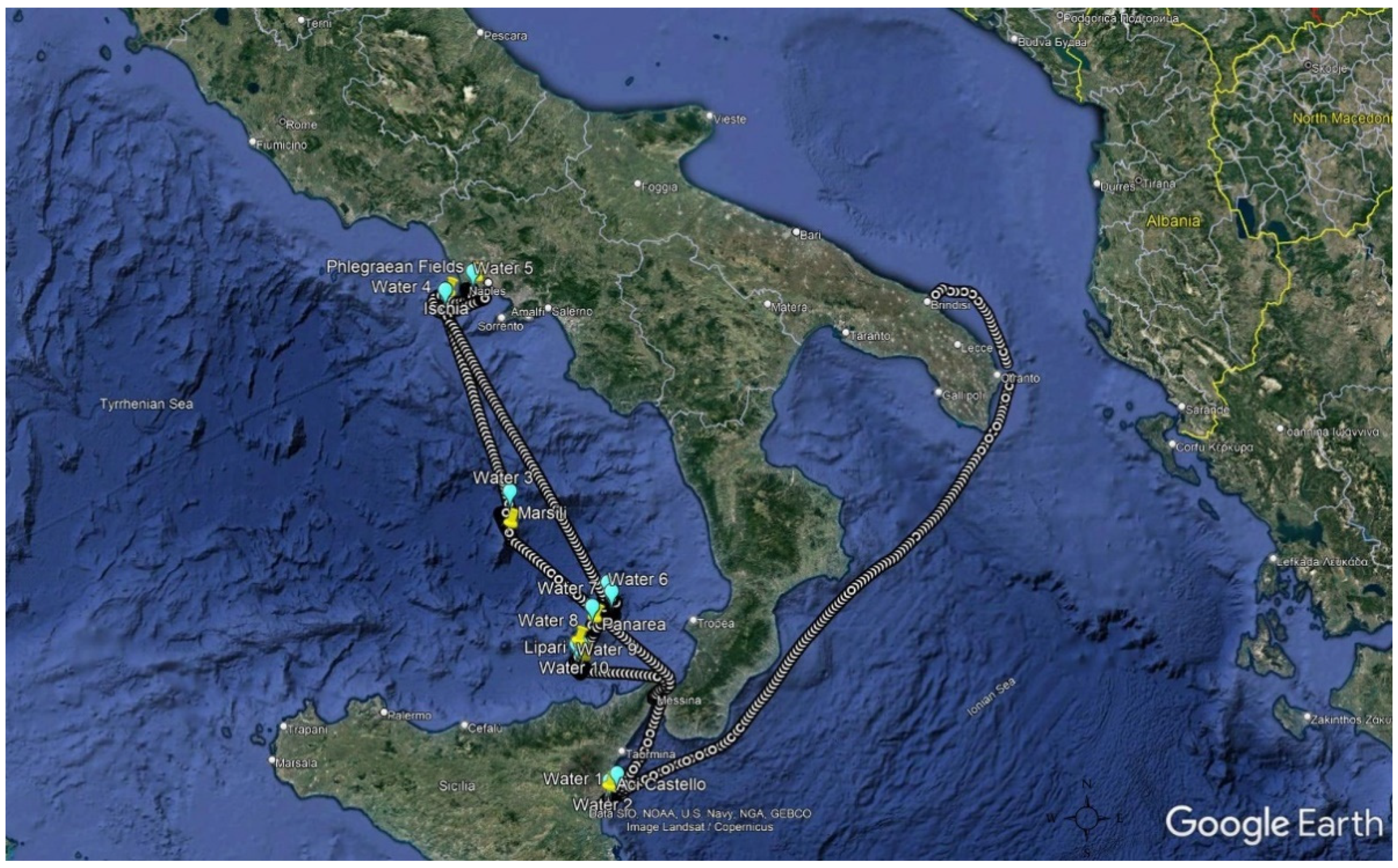
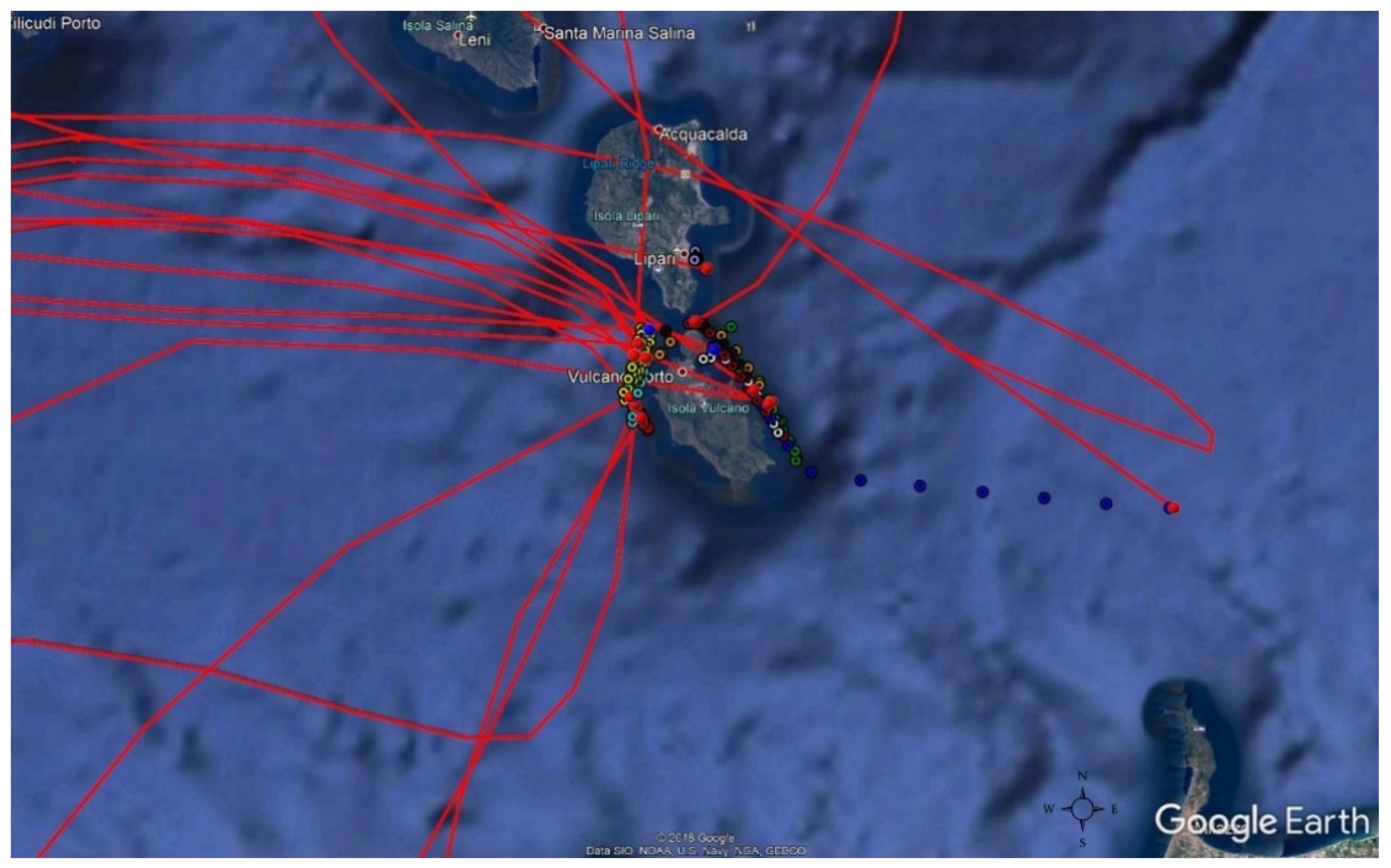
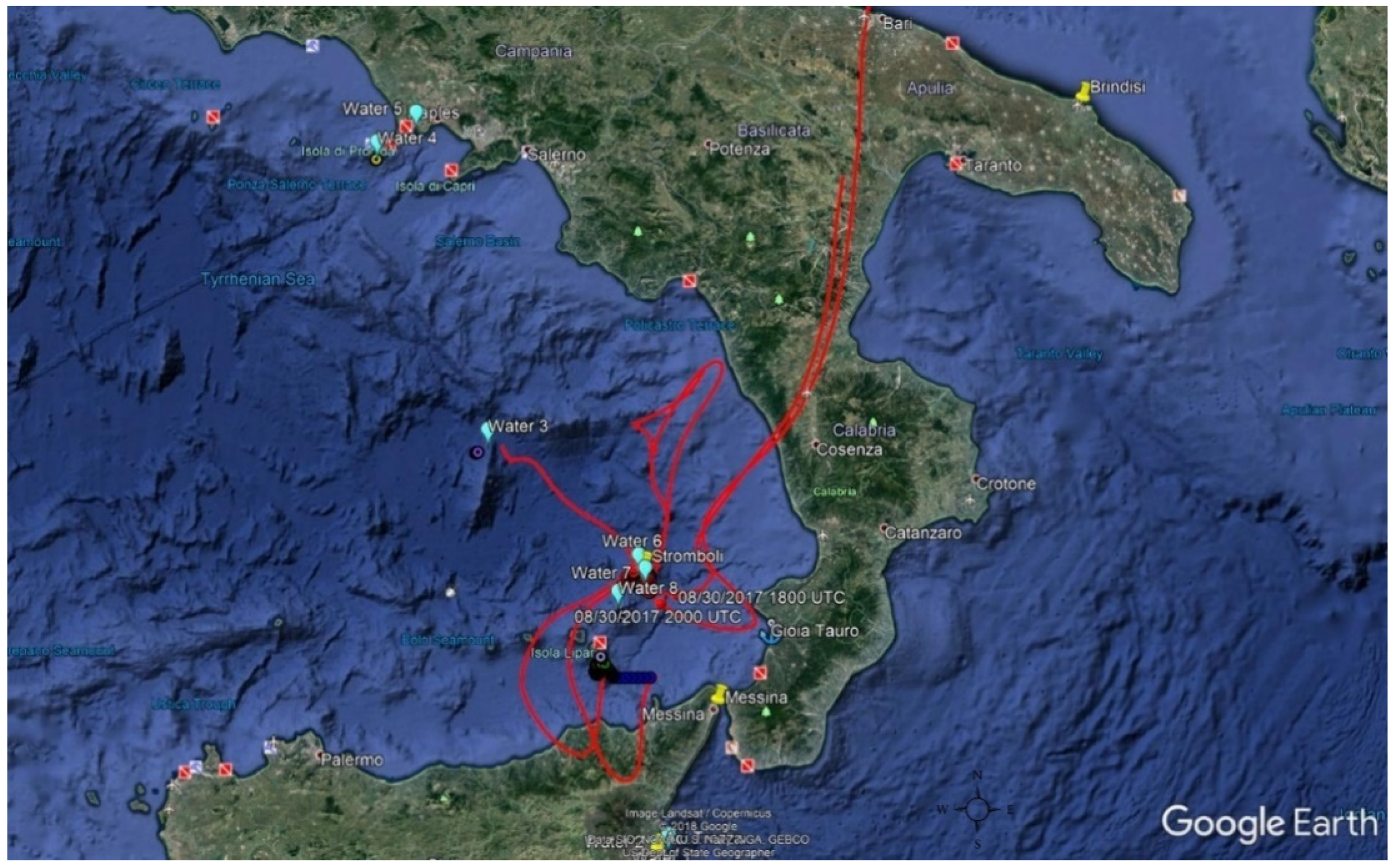
2.1. Scope and Outline of the Study

The cruise, lasting 18 days, started on the 19^th of August 2017 from the Brindisi harbour heading at the southeastern area of the Tyrrhenian Sea and, after touching some hot spots of volcanic and geothermal activity, ended at Messina harbour on the 5^th of September 2017. Details concerning the route are provided in Figure 1.

During the route, the eastern coasts of Sicily overlooking the Etnean area were the first sites monitored. After passing the Aeolian arc, the Tyrrhenian area half a way from the northern Sicilian coasts and Gulf of Naples, in proximity to geologically active seamounts such as Marsili, was also investigated. Then, the research vessel reached the area of Phlegraean Fields and Ischia Island and finally the ship headed back to the Aeolian Archipelago. At the Stromboli and Vulcano islands several passages were performed in order to evaluate local emissions in different conditions in relation both to the time of the day and to meteorological issues. Along the route, as reported in detail in Figures S1 and S2 for the Aeolian area, the VOCs sampling was carried out on a shorter timescale to evaluate more precisely the sources at the Marsili area and at Vulcano, as reported in Tables S1 and S2.

The rationale for sampling times choice was fundamentally based on the need of having a higher time-resolution for VOCs directly emitted from the sources and a daytime/night-time resolution for OVOCs which generally are secondary in origin. Hence each measurement lasted two hours for VOCs and eight hours for OVOCs.

2.2. Sampling

2.2.1. Air Samples Collection

The VOCs sampling was performed by a SKC Model 222-4 pump at a flowrate of 80 mL/min on carbon packed glass traps, described in detail in the following section, able to selectively retain the organic compounds according to their volatility. The VOC sampling traps were homemade by filling glass tubes (15 cm long, 3 mm i.d.), with three subsequent packings containing, in the order, Carbopack C (surface area 15 m²/g), Carbopack B (surface area 100 m²/g), and Carbograph 5 (surface area 500 m²/g) (Lara, Rome, Italy). Quartz wool was used to keep in place the packing material. Before use, the traps were cleaned at 300 °C under a purging flow of helium (100 mL/min, 10 min). Totally 48 samples were collected to assess the concentrations of VOCs other than carbonyls. Sampling periods of 2 h were routinely performed during mornings and evenings of each day of navigation; in addition, intensive measurements were carried out on two days (23rd August; 2nd September), when monitoring was run continuously as reported in Table S1. The sampling time remained equal to 2 h.

Aldehydes concentrations in ambient air were assessed by collecting 35 air samples onto 2,4 dinitrophenylhydrazine (DNPH)-coated silica gel cartridges (7 mm o.d., 110 mm long, SKC, Milan, Italy), meeting the standards [31,32]. The sampling line consisted of a copper coil, (5 m long, 6 mm i.d.) internally coated with KI in order to avoid the measurement bias due to ozone and other oxidants, prior to the cartridge connected to a Bravo Asbesto pump (Tecora, Milan, Italy) set at a flow rate of 340 mL/min. Each DNPH-coated cartridge contained a 300-mg front sorbent section and a 150 mg backup sorbent section, so that breakthrough could be accounted for, and the sampling efficiency could be assessed. The duration of each sampling was of 8 h, day and night hours of each day of navigation were monitored starting respectively from 9 a.m. to 5 p.m. and from 11 p.m. to 7 a.m. of the following day; details are reported in Table S2. During the intensive monitoring days, three eight hours periods were scheduled since a third sample collection was performed in the period from 5 p.m. to 11 p.m.

After sampling, both carbon and DNPH cartridges were closed with tight connectors and kept refrigerated at T < 4 °C in sealed glass containers until the analysis, which was carried out within 30 days after sampling.

During the campaign, one cartridge, handled as those used for sampling, was kept sealed as field blank, and further two cartridges were saved as laboratory blanks, in order to check for possible contamination during the travel.

2.2.2. Water Samples Collection

This study was also extended to the seawater analysis both following the vertical profile employing a Niskin sampling system, not reported in the following, and also sampling shallow waters in the investigated areas to obtain data at the sea–air interface.

Shallow waters were collected, and samples were taken from the sea surface by using 1000 mL quartz Duran bottles properly rinsed three times successively with 15–20 mL of deionized water, dried and then, just prior to sampling, with equal volumes of the seawater to be collected. The samples were divided into separate aliquots and analyzed immediately, to assess the pH and ions concentration, or saved, according to the ISO standard [33], for the successive analysis of the other species to be determined. In the case of metals the sample was acidified at pH = 1–2 and kept refrigerated until the analysis, carried out within a month after the end of the cruise. The samples stored for successive analysis of organic compounds were kept in brown glass vials, properly treated following the specific procedures according to the compounds of interest and kept refrigerated as well.

The last subset of samples was treated with 1.5–2.0 mL of Chloroform (ethanol stabilized from Romil (SPS)) to prevent biological degradation [34]. Details concerning the sampling sites are reported in Figure S1. Totally ten samples were collected from different sites, each divided, as mentioned, in separate subsets.

2.3. Analysis

2.3.1. Air Samples Analysis

The VOCs trapped on the cartridge packed with carbon were thermally desorbed by a Chrompack CP4020 thermodesorber/cryofocuser keeping the liner at first at −180 °C for 3 min while flushing with Helium at 10 mL/min, then raising the temperature to 300 °C under helium (20 mL/min, 10 min) during cryofocusing and injecting the compounds into the column by heating the liner at 300 °C for 1 min in a gas chromatograph (GC-TraceUltra, Thermo, Milan, Italy) connected to a quadrupole mass spectrometer (Trace DSQ-MS, Thermo, Milan, Italy). The analysis was performed by using a VF-1 ms column (50 m × 0.32 mm, 0.40 μm, from Agilent, Milan, Italy), with the following temperature programme (5 °C for 5 min, up to 50 °C in 15 min, then up to 100 °C in 20 min and to 290 °C in 20 min; final isotherm was equal to 5 min). The calibration was achieved by injecting known amounts of the target compounds contained in a certified cylinder (50 ppb of each species in nitrogen, from SIAD, Aprilia LT, Italy). The limit of detection (LOD) for the different classes calculated taking into account the blank values of the unexposed cartridges brought along with the ones employed for sampling, were in the range of 0.10–0.23 μg/m³ for aromatic hydrocarbons and halogenated hydrocarbons and 0.18–0.49 μg/m³ for aliphatic hydrocarbons.

The DNPH cartridges were extracted with 2 mL of acetonitrile and the solutions obtained were analyzed by HPLC (Shimadzu Corporation, Kyoto, Japan) equipped with a photodiode array detector (SPD-M20A) set at a wavelength of 360 nm.

A reversed-phase column Ultra C-18 (100 A, 150 × 4 mm, 5 μm; from Restek, Milan, Italy) kept at 20 °C by means of a column oven (CTO-10AS VP) was used to carry out the separation of the hydrazones derivatives of carbonyls.

The acetonitrile/water mixture (both solvents of Romil Ultra-LC gradient type, 99.9% purity, from Delchimica, Naples, Italy) was used as a mobile phase, and a linear gradient from 40% up to 50% of acetonitrile was applied over 27 min, then held at 100% of acetonitrile for column cleaning; the flow rate was set at 1.0 mL/min.

The aldehydes concentrations were calculated using a multipoint calibration curve (1.5, 1.0, 0.5, 0.25, and 0.15 μg/mL) prepared by diluting standard solutions of the corresponding hydrazones in acetonitrile (Aldehyde/Ketone-DNPH Stock Standard, 1000 μg/mL of each component in acetonitrile, certified reference material, from Sigma Aldrich, Milan, Italy). The amounts of carbonyls found were then corrected taking into account the blanks values. The compounds determined according to the described methodology were C₁-C₁₀ aldehydes and acetone. The LOD for formaldehyde was 0.12 μg/m³ and for acetone was 0.24 μg/m³.

2.3.2. Water Samples Analysis

The shallow waters, collected according to the methodology described before, were analyzed to assess the main parameters and constituents, such as pH, ionic species, and metals. In addition, some organic compounds concentrations were also assessed to improve understanding of the behavior of these compounds in the MBL.

Carbonyl Compounds Analysis

The samples were left at room temperature before extraction, checking the possible presence of particles in suspension and shaken to allow for a better homogeneity.

An amount of 50 mL of aqueous sample was introduced in a flask and 2 mL of citrate buffer (1 M, pH = 3) were added. The pH was adjusted to 3 with HCl. Then 3 mL of DNPH solution were added, and the solution held in agitation was heated at 40 °C for 1 h. The SPE cartridges (Resprep Bonded Reversed Phase, RE 24052, purchased from Restek) were conditioned as suggested by the manufacturer. The volume of the solution was passed quantitatively after letting it cool down. The cartridge was dried under a vacuum, or with nitrogen, and the derivatized aldehydes were eluted with 6 mL of acetonitrile. The volume of the extract was brought to 2 mL under a moderate nitrogen stream. The HPLC-UV analysis at 360 nm was performed successively following the same analytical procedure already described for atmospheric sampling traps analysis.

Acids

The HPLC measurements of organic acids were done on a Shimadzu 10A HPLC system (Shimadzu Corporation, Kyoto, Japan) equipped with a diode array detector, quaternary pump, and degasser and thermostatted column compartment. The column oven temperature was maintained at 25° C and the chromatographic separation was achieved using an Ultra Aqueous C18 (250 × 4.6 mm, 5 µm) column (Restek Corporation, Bellefonte, PA, USA). The isocratic elution was performed with a phosphate buffer solution (50 mM, pH 2.6) as the mobile phase. The flow rate was maintained at 1 mL/min and the injection volume was 20 µL. Detection was in wavelength range of 190–230 nm for malic, maleic, succinic, lactic, and oxalic acids. The peaks were identified by their retention times, comparing the UV–Visible spectra and spiking with standards. Quantification has been done using an external standard curve with six different concentrations of organic acid standard solutions (0.01, 0.1, 0.25, 0.5, 1000, and 2000 ppb for all organic acids). Each calibration sample was analyzed in triplicate.

Formic, acetic, and methanesulphonic acids were analyzed by IC (DX-120, Dionex, Sunnyvale, California, USA) equipped with an AS4 column, AG4 guard column, an ASRS-Ultra anion self-regenerating suppressor, and a conductivity detector. Tetraborate eluent (1.25 mM Na₂B₄0₇) was used [35] with an injection volume of 150 µL. The calibration curves were constructed with six standard solutions (0.01, 0.1, 0.25, 0.5, 1000, and 2000 ppb for three organic species). Each standard/sample was analyzed in triplicate.

Anions & Cations

The analysis was performed through ion chromatography (IC) (ICS 1000, Dionex, Sunnyvale, California, USA) equipped with an AS12A column and AG12A guard column, an ASRS-Ultra anion self-regenerating suppressor, and a conductivity detector, after the opportune dilution of the seawater samples. The analysis was performed by isocratic eluition at a flow rate of 1.5 mL/min using 0.3 mM NaHCO₃ and 2.7 mM Na₂CO₃ eluent, the injection volume was 50 μL. The amounts of anions (fluoride, chloride, bromide, sulphate) and cations (Sodium, Potassium, Magnesium, Calcium) were determined referring to calibration curves constructed with water solutions prepared by dilution of stock standards (Certipur from Merck, Milan, Italy) containing 1000 mg/l of each analyte.

Metals

Opportune dilutions (1:100, 1:200, 1:1000) of the samples collected were made with Ultrapure water to avoid the effect of species such as Sodium and Magnesium which are present at high concentrations. The samples were marked with an internal standard of Yttrium, Lanthanum, and Erbium.

An ICP-MS Agilent model 7700 equipped with an autosampler was used to run the analyses. First in the tuning phase the instrumental response was assessed with a standard solution, then the optimal configuration found in the tuning was saved in the method set up. The calibration lines of the analytes of interest were later acquired using the same method.

The six-points calibration curve (0-5-10-25-50-100 ppb) was obtained by the opportune dilution of a multielement standard solution at 10 ppm (V for ICP purchased from Fluka) and an arsenic standard at 10 ppm (Fluka Arsenic Standard for ICP). The calibration solutions were marked with the same internal standard (mixture of Yttrium, Lanthanum, and Erbium) which has been added to the samples to be analyzed.

2.4. Continuous Inorganic Gaseous Pollutants Measurements

The monitoring of gaseous pollutants throughout the cruise was performed by automatic analyzers. The O₃ measurements were carried out using the automatic UV Teledyne Photometric Ozone Analyzer (API Model 400E, San Diego, California, USA) on the top deck (about 10 m a.s.l.), the sampling flow rate was 0.8 l/min with a time resolution of 1 min. The NO_x observations were performed by a Teledyne Nitrogen Oxides Analyzer (API Model 200E, San Diego, California, USA) with a sampling flow rate of 0.5 l/min and a time resolution of 1 min. The SO₂ measurements were performed using the fluorescence method by a Teledyne UV Fluorescence SO₂ Analyzer (API Model 100E, San Diego, California, USA) with a sampling flow rate of 0.6 l/min and a time resolution of 1 min. All these analyzers were calibrated at the beginning of the measurement.

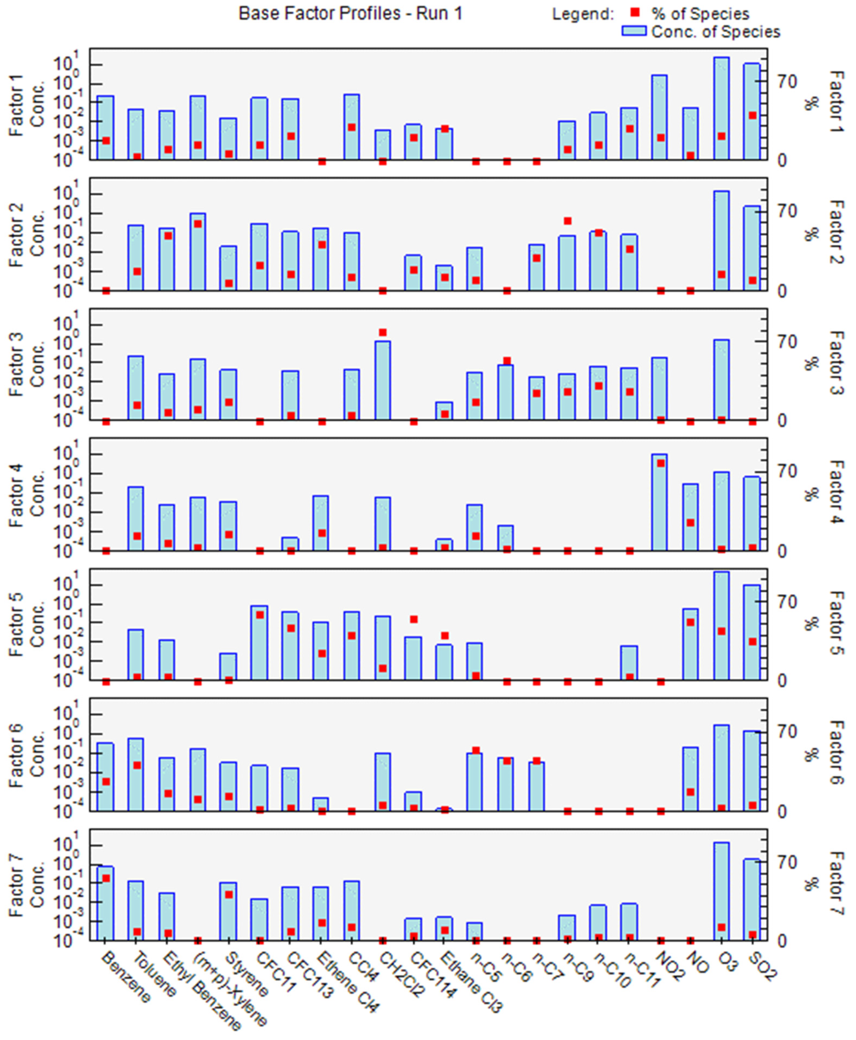
2.5. Statistical Treatment on the Dataset by PMF Model

To comprehensively consider the dataset gathered through the Med-Oceanor 2017 campaign, aiming at identifying the different sources contribution, a statistical treatment was performed by using the PMF (Positive Matrix Factorization). This receptor model developed by Paatero and Tapper [36] is now widely recognized and accepted as a data analysis tool. This model has an extensive range of applications, since it is frequently employed to study the sources of Particulate Matter (both as PM₁₀ and PM_2.5) [37], and also to VOCs data [38,39].

The software freely made available by EPA (EPA PMF 5.0.14) was applied to the dataset comprising all of the volatile organics (except for aldehydes which were averaged on a different time period) and inorganic pollutants such as NO₂, NO, O₃, and SO₂.

The PMF model is run by the user inputting the concentration data of each sample with the associated uncertainty calculated as reported in many studies [38,39]. The PMF decomposes the data matrix X, of dimensions i (number of samples) and j (number of the measured chemical species), into two matrices G (source contribution, of dimensions p and i) and F (source factors, of dimensions p and j). The Objective function Q is defined as:

$$\mathrm{Q}={{\displaystyle \sum }}_{i=1}^n{{\displaystyle \sum }}_{j=1}^m{\left[\frac{\left(X_{ij}-{{\displaystyle \sum }}_{k=1}^p{g}_{ik·}{f}_{ik}\right)}{u_{ij}}\right]}^2$$

(1)

where k = individual sources, u_ij = measurement uncertainties, n = total number of samples, and m = total number of species; through the residual matrix, in round brackets, and u_ij, the PMF minimizes the function Q. According to the datapoints considered, the function Q can be distinguished in: Q_true if it comprises all data points, Q_robust if outliers are excluded, and Q_theo which equals the number of degrees of freedom.

The ratio Q_true/Q_theo and Q_true/Q_robust expresses the goodness of fit for a given number of factors, the optimal value is close to 1.

3. Results and Discussion

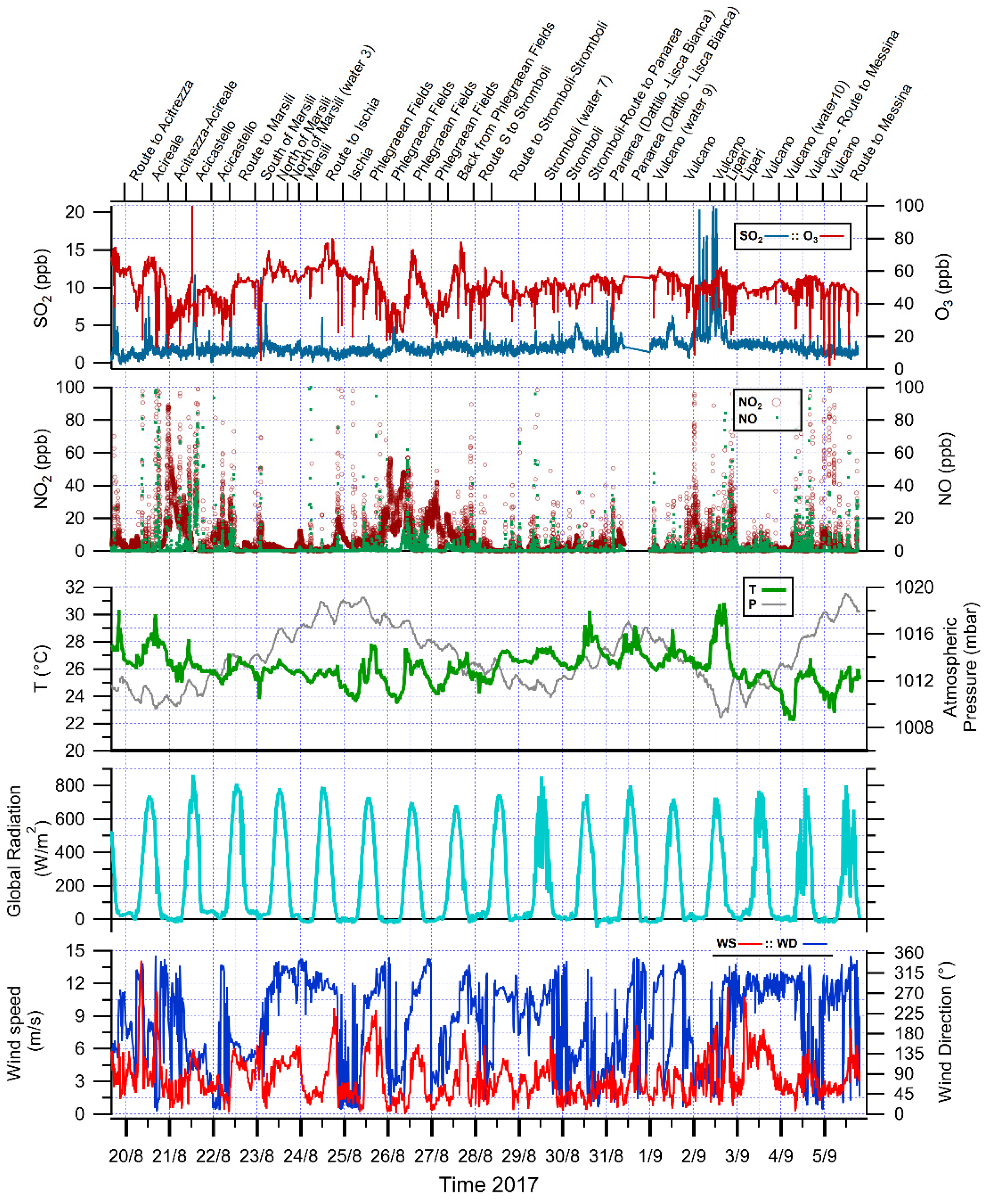
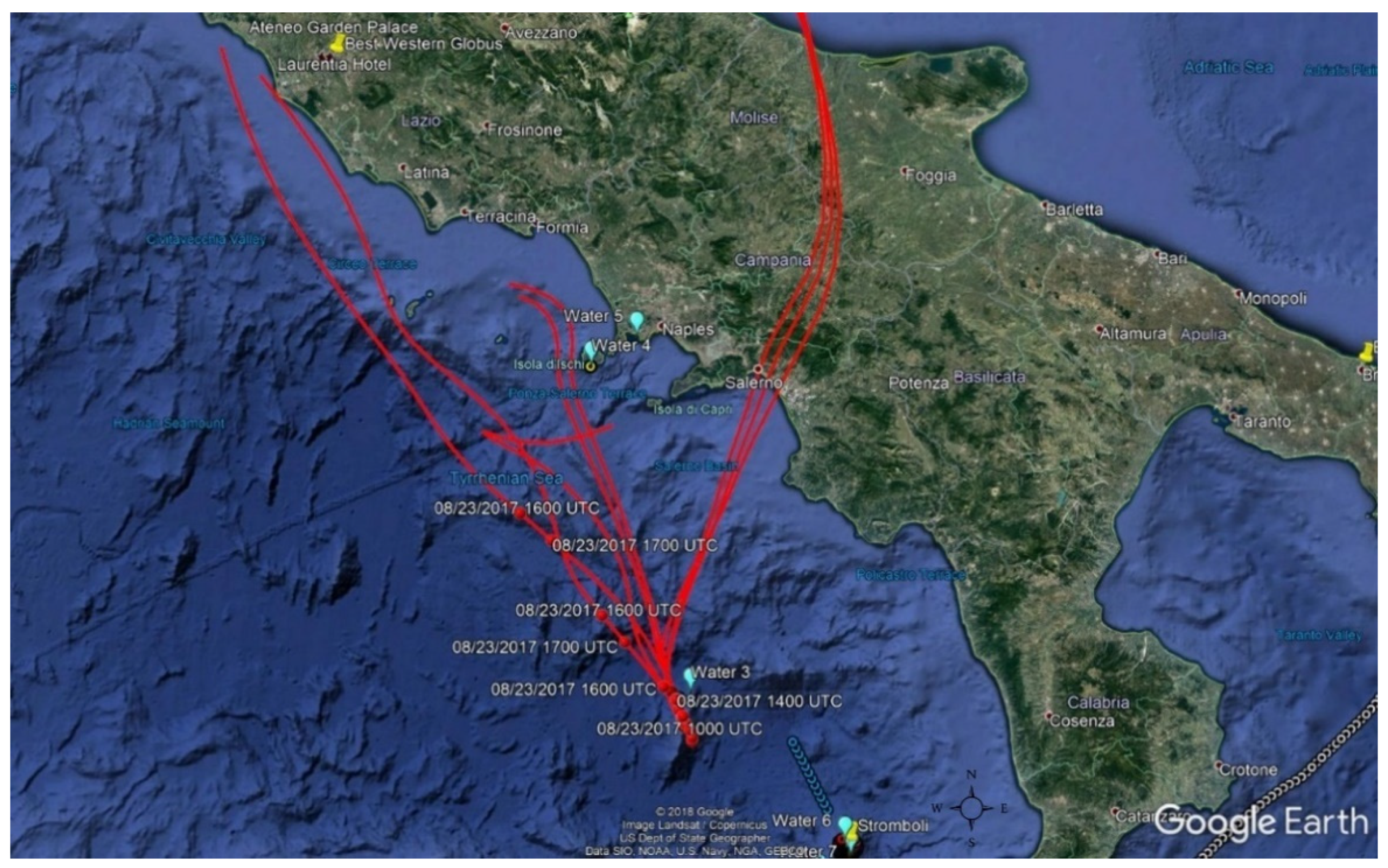
3.1. Meteorology of the Period

The diurnal variations in meteorological parameters are shown in Figure 2 together with those of gaseous pollutants. The period investigated was, as expected, hot and dry. During the cruise the mean temperature was 26.1 °C and the atmospheric pressure was 1014.05 mbar.

Generally, the Global radiation values had a well-defined diurnal trend peaking between 10:00 and 12:00 and reaching higher values of about 860 W/m² on the 29^th of August.

A mean wind speed of 3.3 m/s was calculated on the whole period data, hence mild breezes were present. The prevalent wind direction was from NNW-N (36% of the data), winds from NE-S and S-NW directions were recorded respectively for about 23.4% and 24.5% of the data and, finally, less frequently from the N-NE (16%). The stronger winds, with a speed of 13–14 m/s, were observed during the early morning of the 20^th of August and in the late afternoon of the 2nd of September, when a maximum value of 11.7 m/s was recorded. A single storm event, which forced the ship to recover at Lipari, occurred on the 2nd of September, as also shown by the sharp decrease in temperature.

A detailed analysis of wind records is necessary in order to better understand the impact of local sources and to focus on volcanic contribution. Some of the hot spots, intensively monitored along the route, were examined in such detail.

By the analysis of windroses plotted on Vulcano Island (Figure S3) it is possible to observe that the winds usually came from the land both on eastern and western coasts, with a few exceptions. In the case of Stromboli island the winds usually came from the sea.

The analysis of wind data was performed in combination with backward trajectories available by running the Hysplit model through the NOAA ARL website (http://www.arl.noaa.gov/ready/ accessed on 7 July 2021) [40].

3.2. General Observations on Gaseous Pollutants Dataset

Table 1. Basic statistical parameters calculated for the automatic analyzers’ dataset (µg/m³).

Pollutant	Mean	SD	Variance	RSD	Min	Median	Max
NO2	13.7	13.4	179.4	1.0	1.0	8.8	51.7
NO	1.8	1.7	2.9	0.9	0.6	1.3	7.1
O3	103	10.4	108	0.10	77.4	104	126
SO2	25.9	5.30	28.0	0.20	20.6	25.2	46.6

shows a statistical overview of all NO, NO₂, O₃, and SO₂ concentrations over the whole sampling period. It is possible to observe that, as expected, some differences can be found among differently anthropized areas and also on the basis of nearby natural sources. The highest NO₂ concentrations were found in proximity to Sicilian coasts and to Phlegraean Fields (Figure 2). Occasionally, peaks were also found in the Aeolian area nearby Vulcano. It happened on the 2nd September during the first measurement of the intensive campaign and on the 4^th of September morning measurement. The former peak could likely be ascribed to aged air masses, coming from the Gulf of Tunis according to the backward trajectory, since the ozone concentration is below the average levels found during the succeeding nocturnal measurement. The following NO₂ peak recorded is mirrored by the total hydrocarbons which in turn show an appreciable peak. In this case the backward trajectory passes through Vulcano Island before reaching the monitoring point. The same correspondence can be noticed for the NO₂ peak measured at Ischia Island. Generally speaking, both the Sicilian coasts at the beginning of the cruise and the Phlegraean Fields showed increased NO₂ concentrations with respect to other sites. A clear increasing trend can be recognized for SO₂ in the last part of the cruise (about 24% of increase), in the Aeolian area, particularly near Vulcano and Lipari.

The ozone levels measured throughout the cruise were those typical of the seasonal period investigated [1,41] which in the Mediterranean basin is usually associated with high photochemical pollution. The observations made during the cruise agree with a previous work [42] which referred to the same geographic area of the Mediterranean basin. Mild day–night changes of the pollutant concentrations were detected especially when the ship was in the open sea. At Marsili site on the 23rd of August no day–night trend was observed at all. The highest ozone concentrations were measured during sailing in this area likely due, as the backward trajectory indicate, to the precursors punctual sources of Rome and Naples as already observed by Velchev et al. [42].

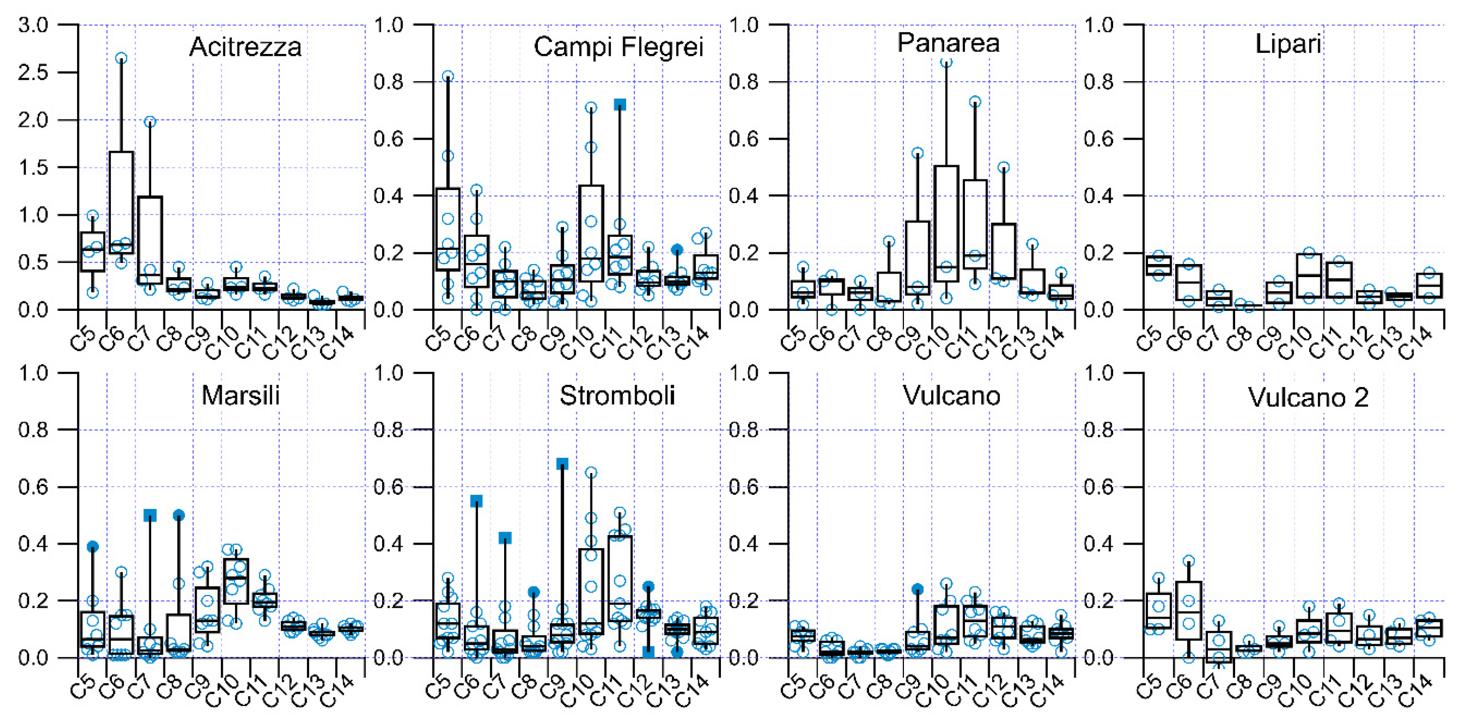
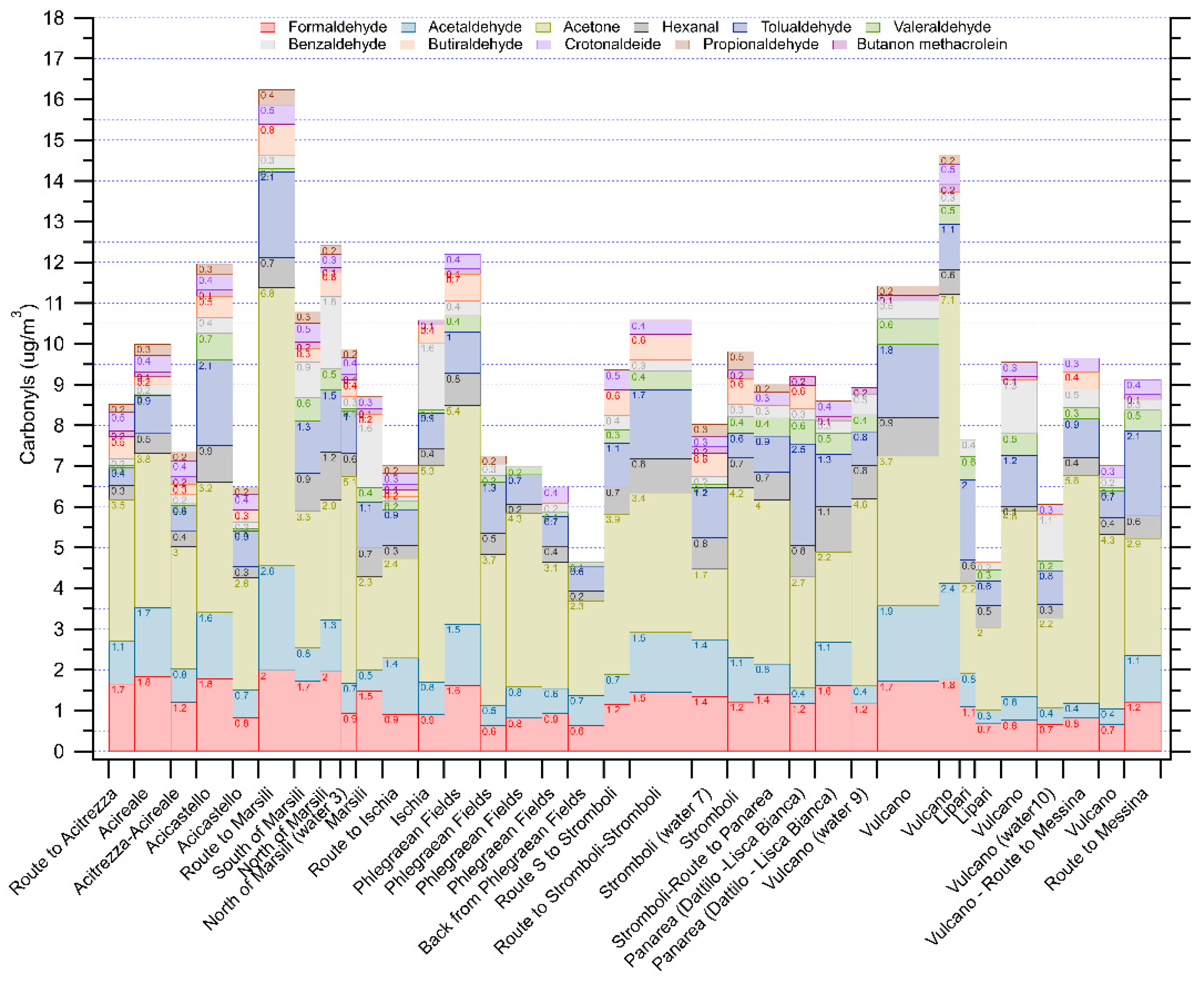
3.3. Volatile Organic Compounds Concentration Distribution over the Area

The organic compounds over the investigated area showed average values, reported in

Table 2. Basic statistical parameters calculated for the hydrocarbons’ dataset (µg/m³).

Pollutant	N Tot	Mean	SD	Variance	RSD	Min	Median	Max
Benzene	48	1.47	1.32	1.74	0.89	0.34	1.11	7.26
Toluene	48	1.79	1.85	3.42	1.03	0.44	1.07	9.07
Ethyl Bz	48	0.44	0.43	0.18	0.97	0.11	0.32	2.88
(m+p)-Xylene	48	1.60	1.09	1.18	0.68	0.46	1.21	4.90
o-Xylene	48	0.54	0.49	0.24	0.91	0.14	0.36	2.93
Styrene	48	0.32	0.28	0.08	0.89	0.02	0.22	1.12
CFC11	48	1.13	0.64	0.41	0.57	0.12	1.01	3.06
CFC113	48	0.73	0.20	0.04	0.28	0.25	0.78	1.18
C2Cl4	48	0.39	0.34	0.12	0.88	0.01	0.28	1.85
C2HCl3	48	0.09	0.05	0.00	0.61	0.02	0.07	0.21
CCl4	48	0.90	0.28	0.08	0.31	0.00	0.94	1.62
CHCl3	44	0.71	0.84	0.70	1.17	0.02	0.34	3.28
CH2Cl2	45	1.66	2.03	4.12	1.22	0.02	0.56	6.81
CFC114	48	0.03	0.02	0.00	0.57	0.00	0.03	0.10
C2H3Cl3	48	0.02	0.01	0.00	0.35	0.00	0.02	0.03
n-C5	48	0.21	0.23	0.05	1.10	0.01	0.12	0.99
n-C6	48	0.38	0.86	0.74	2.28	0.00	0.11	4.37
n-C7	48	0.15	0.33	0.11	2.14	0.00	0.05	1.98
n-C8	48	0.09	0.11	0.01	1.29	0.01	0.03	0.50
n-C9	48	0.12	0.13	0.02	1.05	0.02	0.10	0.68
n-C10	48	0.23	0.22	0.05	0.98	0.02	0.17	1.11
n-C11	48	0.21	0.15	0.02	0.73	0.04	0.18	0.73
n-C12	48	0.12	0.07	0.01	0.61	0.02	0.12	0.50
n-C13	48	0.09	0.04	0.00	0.46	0.02	0.09	0.23
n-C14	48	0.10	0.05	0.00	0.49	0.02	0.10	0.27

, similar to those assessed in the same season in other works. The value of n-pentane, n-hexane, n-heptane, and n-octane reported were respectively 0.41 µg/m³, 0.34 µg/m³, 0.13 µg/m³, and 0.22 µg/m³, whereas lower values were measured for benzene (0.38 µg/m³) and toluene (0.53 µg/m³) [43].

Aliphatic hydrocarbons over the investigated area at coastal sites more heavily impacted by anthropic sources, such as the Sicilian coasts and Gulf of Naples sites, showed the highest values evenly distributed in C5-C9 and C10-C14 classes.

Different aliphatic hydrocarbons profiles were observed at different sites, the data distribution according to the site is reported in the form of boxplots (Figure 3).

The C10 and C11 were abundant in all the samples, with only few exceptions, but the trends shown by remote areas and anthropogenically impacted sites (Sicilian coasts, Phlegraean Fields) are somehow different. A bimodal distribution with maxima at C5–C6 and C10–C11 could be observed for the latter, whereas a unimodal distribution with maxima at C10–C11 is shown by the former (Marsili, Stromboli, Panarea, Vulcano). The predominance of heavier n-alkanes in the marine environment has already been reported [44] and the data obtained during the cruise generally agree with the previous studies. As well-known [45,46] the ability of these compounds to react with OH radicals increases with the chain length, therefore their predominance should likely be ascribed to the presence of local sources. On the other hand, comparing the different sampling periods, especially during the intensive measurements, a clear decreasing trend could be observed approaching night-time.

A few exceptions to these observations are represented by two intensive measurement periods around the Marsili area on the 23rd of August early morning (09:00–11:00) and late night (22:40–00:40), in both the cases aliphatic hydrocarbons profiles followed a bimodal distribution. As for the trends obtained site by site, a deeper analysis can be attempted. At the Marsili site, the first three sampling periods are characterized by air masses coming from the land, whereas the following samplings were impacted by central Tyrrhenian upcoming air masses (see Figure 4). In the first case a bimodal distribution was observed, for the other samplings during the 23rd of August afternoon the distribution was unimodal.

Other site-dependent observations of peculiar hydrocarbons profiles concern the increased C5–C7 percentage of alkanes on the total (C5–C14) sampled in proximity to Sicilian coasts (66%), with respect to the average values during the whole cruise (41%).

The measurements also included carbonyls, collected on an 8-h basis during the day and the night, their average values and other statistical parameters are reported in

Table 3. Basic statistical parameters calculated for carbonyls’ dataset (µg/m³).

	N Tot	Mean	SD	Variance	RSD	Min	Median	Max
Formaldehyde	34	1.23	0.43	0.18	0.35	0.63	1.20	1.99
Acetaldehyde	34	0.99	0.56	0.32	0.57	0.33	0.81	2.57
Acetone	34	3.66	1.32	1.75	0.36	1.72	3.45	7.09
Acrolein	0	--	--	--	--	--	--	--
Propionaldehyde	16	0.26	0.07	0.01	0.29	0.19	0.23	0.46
Crotonaldehyde	24	0.37	0.07	0.01	0.20	0.25	0.37	0.51
2-Butanon-methacrolein	22	0.13	0.05	0.00	0.41	0	0.14	0.23
Butiraldehyde	19	0.46	0.18	0.03	0.39	0.16	0.52	0.75
Benzaldehyde	33	0.48	0.46	0.22	0.96	0	0.31	1.78
Valeraldehyde	34	0.31	0.20	0.04	0.66	0.04	0.31	0.66
Tolualdehyde	34	1.16	0.52	0.27	0.45	0.43	1.03	2.49
Hexaldehyde	34	0.60	0.26	0.07	0.44	0.11	0.57	1.18

. Among the carbonyls the most abundant compound was acetone with an average value of 3.66 μg/m³, accounting for 38% of the total amount collected, and formaldehyde and acetaldehyde with average values respectively of 1.23 μg/m³ and 0.99 μg/m³ made up about 22–29% depending on the site.

These findings are consistent with measurements performed in the same period (from the end of June to the end of August 2017) by Wang et al. [47] in the AQABA campaign, aimed at finding atmospheric organic pollutants distribution over a wide route. The cruise started from southern France and ended in the Mediterranean Sea after passing through the Suez Canal and circumnavigating the Arabian Peninsula. The concentrations found in the Mediterranean Sea (no further details are given concerning the specific sites) were comparable to those found in the present study in the same period. The acetone also in that case was the dominant species with a concentration of more than 2 ppb (4.74 µg/m³), followed by a formaldehyde of 0.86 ppb(1.05 µg/m³) and acetaldehyde of 0.30 ppb (0.54 µg/m³).

The percentage increased if the site was more impacted by anthropic sources.

In Figure 5 it is possible to observe that the trend characterizing the total load of carbonyls measured showed a good agreement with the single predominant aldehydes (formaldehyde and acetaldehyde). Inside the bars the concentration value of the single compounds is also reported.

A particular trend is shown by the benzaldehyde which has the highest relative standard deviation since, apart from the maxima, exceeding 1 µg/m³, found at Marsili, on the way to Ischia and at Lipari, the average value found for the rest of the cruise was of 0.30 µg/m³. The maxima were accompanied in some cases by high levels of hydrocarbons (23rd August diurnal and 24^th August nocturnal measurements), and on the 3rd of September and the 4^th of September data the trend of this aldehyde was similar to the one of tolualdehyde. It is possible to consider diagnostic ratios such as C1/C2 which can be used as an indication of photo-oxidation, and the C2/C3 ratio of the anthropogenic origin, as reported in many works [48,49]. The values calculated (reported in

Table 4. Diagnostic ratios calculated for carbonyls’ dataset.

OVOC Sample	Sampling Area	C1/C2	C2/C3
1	Route to Acitrezza	1.58	5.39
2	Acireale (water 1)	1.09	6.13
3	Acitrezza-Acireale	1.48	3.61
4	Acicastello (water 2)	1.10	6.10
5	Acicastello (water 2)	1.22	3.57
6	Route to Marsili	0.77	6.90
7	South of Marsili	2.09	2.77
8	North of Marsili	1.53	5.80
9	North of Marsili (water 3)	1.27	3.45
10	Marsili	2.91
11	Ischia	0.68	7.28
12	Ischia western coast (water 4)	1.14
13	Phlegraean Fields Pozzuoli Gulf (water 5)	1.09
14	Phlegraean Fields Pozzuoli Gulf (water 5)	1.23	2.48
15	Phlegraean Fields Pozzuoli Gulf (water 5)	1.05
16	Phlegraean Fields Pozzuoli Gulf (water 5)	1.50
17	Backward Route from Phlegraean Fields	0.87
18	Route southwards to Stromboli	1.59
19	Stromboli (water 6)	0.99
20	Stromboli
21	Stromboli (water 7)	0.96	4.53
22	Stromboli 1	1.12	2.37
23	Stromboli-Route to Panarea	1.86	3.43
24	Panarea (between Dattilo and Lisca Bianca)	3.07
25	Panarea (between Dattilo and Lisca Bianca)(water 8)	1.51
26	Vulcano (water 9)	2.65
27	Lipari	0.93	8.16
28	Lipari
29	Lipari	0.75	11.23
30	Lipari	1.36
31	Vulcano	2.07
32	Vulcano (water 10)	1.34
33	Vulcano—Route to Messina	1.67

) suggest that during the first part of the cruise the anthropogenic origin is predominant over the secondary production, this is also evident from the values of propionaldehyde, usually associated with anthropogenic emissions, which are for the most part of the cruise below the detection limit. The average value of the C2/C3 in the Acitrezza area and at Marsili is 4.8, not much different than the one reported for urban areas [50]. During the rest of the cruise the C2/C3 ratio was sometimes high, as in the case of Ischia and Lipari, as if it was associated with natural precursors.

The average C1/C2 ratio through the whole cruise was about 1.5 which, according to Shepson et al. [51], is normally found in urbanized areas. Peak values of this ratio higher than 2.5 were found at Marsili, Panarea, and Vulcano.

Among the organic compounds, the CFCs class was also considered to evaluate the potential emission from volcanic sources, as reported by Schwandner et al. [16]. In the cited work the data are referred to the measurements made at the emission points and are reported for the different kind of source (diffuse emissions, fumarolic gases, etc). Nine compounds were quantified (as reported in Table 2), among them dichloromethane and trichlorofluoromethane (CFC11) were the most abundant. The CFC11 was plotted against a toluene to benzene ratio (Figure S4) since, based both on Frische et al. [18] and on Schwandner et al. [16], it can be considered, among the halogenated compounds, as a tracer of geogenic emissions. Although on the whole the correlation between toluene to benzene ratio and CFC11 is poor (R² = 0.56), the agreement between the trends increased during the route through the Aeolian Islands (R² = 0.75) and especially during the Vulcano intensive campaign on the 2nd September (R² = 0.81).

Analyzing CFC11 peaks exceeding 1.29 µg/m³, the average atmospheric level in the northern hemisphere [46,52], it was apparent that levels above the average were found in the area of Ischia and in some sporadic measurements around Stromboli and Vulcano (Figure S4). Trying to better characterize the general conditions affecting these measurements through backward trajectories analysis and wind records, no evidence could be found of a geogenic influence. By analyzing 24 hrs backward trajectories (in Figure 6 and Figure 7) it appeared clear that, apart from local air circulation patterns, massive air movements at the two coasts of Volcano were different in origin, being the western coast was mainly impacted by air masses coming from the sea, whereas the air masses frequently passed over the island, more or less near the volcanic area, before getting to the eastern coast. The VOC sample nr. 41 was apparently more impacted by air masses coming from the volcanic area brought by local winds and longer-range transport, a CFC11 value of 1.86 µg/m³ was found during the measurement at this site. On the other hand, sample nr. 38 showed peculiar features since, even if it was collected with stronger winds coming from land, it was also subject to the influence of air masses passing through the northeastern Sicilian coast. It had a low value of CFC11 (0.49 µg/m³) and a high SO₂ concentration value (46.6 µg/m³). Opposite observations were made for sample nr. 45 impacted by seaward winds and by air masses coming from Vulcano Island which showed an intermediate CFC11 value of 1.15 µg/m³.

On the whole, the mean CFC11 value measured throughout the cruise was 1.13 µg/m³, lower than the average atmospheric level.

3.4. Water Samples Measurements

Shallow water was also collected during the cruise as already described in Section 2.1. at the sites listed in Table S3.

Basic measurements of pH, ionic content, metals, carbonyls, and organic acids were performed on the sea water samples.

The results of pH measurements and ionic composition determined by ion chromatography are reported in

Table 5. pH values and ionic composition of the samples (mmol/Kg).

Sample	pH	F#x2212;	Cl−	Br−	SO42−	F#x2212;/Cl#x2212; (·10^−5)	Na+	Mg2+	K+	Ca2+
water 1	8.60	0.03	688.74	0.81	30.77	4.09	476.03	53.74	9.53	9.37
water 2	8.62	0.04	298.39	0.36	12.86	12.19	522.22	59.37	10.30	10.20
water 3	8.52	0.09	591.69	0.72	25.30	15.33	523.86	60.61	10.81	10.83
water 4	8.55	0.05	561.93	0.68	25.08	9.67	523.44	59.68	10.34	10.53
water 5	8.59	0.03	767.80	0.95	35.04	4.07	565.67	64.46	11.12	10.62
water 6	8.59	0.04	448.30	0.58	19.28	8.00	513.39	58.91	15.29	9.72
water 7	8.57	0.03	450.12	0.57	18.87	6.72	510.97	58.89	10.35	9.67
water 8	7.70	0.11	223.99	0.26	9.55	48.73	494.45	55.99	10.32	9.35
water 9	8.58	0.08	117.41	0.18	5.08	72.02	476.09	54.10	9.65	9.31
water 10	6.92	0.08	302.93	0.43	12.73	25.38	524.09	59.37	10.22	10.40
average	8.32	0.06	445.13	0.55	19.46	20.62	513.02	58.51	10.79	10.00

. The pH value found was on the average around 8.3, similar to the value of 8.1, typical of Mediterranean area [53], whereas samples 8 and 10 had a value lower than the average. Sample 8 was collected north of Panarea Island. A geothermic contribution was hypothesized for both the samples since submerged seeps were recently documented in the area. The submarine hydrothermal system of Panarea Island is 70 km² wide and it includes active vents marked by intense discharge of CO₂-dominated gases and thermal fluids with temperatures as high as 140 °C [54]. There was a similar situation for sample 10 which was taken at Levante Bay in the northeastern side of Vulcano Island, where gas vents are also located as reported by Boatta et al. [55].

As expected the major ions were Na⁺, K⁺, Ca²⁺, Mg²⁺, Cl⁻, SO₄²⁻, being Br⁻ and F⁻ minor species. The concentrations determined were in good agreement with previous studies carried out in the same area [56] and also elsewhere [57]. The F⁻/Cl⁻ molal ratio was calculated, since the geothermic contribution to the enrichment in F⁻ was previously reported for seawater [56] and for precipitations [57] in proximity to volcanic areas. The highest ratios found at water 8 and 10 could also likely explain, at least in part, the increased acidity of the samples showing the lowest pH. A contribution to this lowering, mainly caused by CO₂, could also probably come from hydrofluoric acid (HF).

The metals content of the seawater was also a subject of the study (see

Table 6. Metallic composition of the samples (µmol/Kg).

Samples	Li	Be	Al	V	Cr	Mn	Fe	Co	Ni	Cu	As	Rb	Sr	Cs	Pb
water 1	34.8	0.3	2.1	0.6	0.1	0.1	8.0	0.1	0.2	0.2	0.8	1.6	103.7	0.02	0.01
water 2	35.4	0.3	2.7	0.6	0.1	0.1	10.2	0.1	0.2	0.2	0.7	1.6	103.3	0.02	0.01
water 3	36.4	0.2	1.8	0.6	0.1	0.1	12.5	0.1	0.2	0.2	0.6	1.7	104.5	0.02	0.01
water 4	36.5	0.3	2.1	0.6	0.1	0.1	13.9	0.1	0.2	0.2	0.6	1.7	105.7	0.02	0.01
water 5	38.0	0.3	2.9	0.6	0.2	0.2	16.3	0.1	0.2	0.2	0.5	1.8	107.6	0.03	0.01
water 6	37.1	0.1	1.0	0.6	0.1	0.1	17.4	0.0	0.2	0.1	0.4	1.7	107.2	0.02	0.00
water 7	39.3	0.3	2.5	0.6	0.2	0.1	15.8	0.1	0.2	0.1	0.5	1.7	105.7	0.02	0.01
water 8	31.0	0.0	1.0	0.7	0.2	0.1	37.0	0.0	0.1	0.2	0.3	1.6	97.9	0.01	0.01
water 9	30.4	0.0	1.3	0.7	0.2	0.1	35.6	0.0	0.2	0.2	0.3	1.6	95.2	0.01	0.01
water 10	35.0	0.0	2.6	0.8	0.2	1.4	43.3	0.0	0.2	0.2	0.3	2.0	104.1	0.03	0.00
average	35.4	0.2	2.0	0.6	0.2	0.2	21.0	0.1	0.2	0.2	0.5	1.7	103.5	0.02	0.01

).

The first observations arising from the metals’ dataset confirm that the last three samples collected in the Aeolian area showed higher levels of Iron, and the last sample also of Manganese and Rubidium. As reported by Elderfield et al. [58] both Manganese and Iron are diagnostic of vent activity.

The analysis on the samples collected also included several organic compounds: both lower weight carbonyls and some organic acids, including dicarboxylic acids were quantified as reported in

Table 7. Carbonyls’ content of the samples (nM).

Sample	Formal- dehyde	Acetal- dehyde	Acetone	Benzal- dehyde	Valeral- dehyde	Tolual- dehyde	Hexal- dehyde
water 1	8.77	8.03	25.22	0.04	1.03	3.87	0.43
water 2	6.17	13.14	22.84	0.09	0.53	4.37	0.00
water 3	4.29	1.88	15.87	0.00	0.15	5.20	0.00
water 4	6.31	10.69	25.91	0.00	0.88	4.45	0.00
water 5	5.96	27.78	5.84	0.04	0.76	6.48	0.00
water 6	5.55	14.69	12.76	0.00	0.37	5.29	0.00
water 7	10.87	22.61	31.49	0.00	2.77	1.77	0.00
water 8	1.62	25.80	13.49	0.00	2.06	0.97	0.00
water 9	17.33	30.38	32.26	0.00	0.68	5.97	3.34
water 10	24.48	27.17	23.21	0.00	0.62	6.14	0.68
average	9.14	18.22	20.89	0.02	0.98	4.45	0.45

and

Table 8. Organic acids content of the samples (nM).

Sample	Formic Acid	Acetic Acid	Oxalic Acid	Succinic Acid	Malic Acid	Maleic Acid	Lactic Acid	Methane- Sulphonic Acid
water 1	7.717	32.73	281.2	0.000	4.567	0.207	3.297	34.56
water 2	9.196	56.83	270.6	0.000	5.261	0.198	3.364	24.01
water 3	2.848	16.53	231.6	0.000	0.955	0.172	7.527	55.91
water 4	12.45	0.65	229.1	0.000	0.918	0.190	3.552	32.60
water 5	6.978	0.33	217.0	0.000	3.418	0.422	3.841	16.16
water 6	4.652	17.22	264.3	3.229	11.10	0.216	7.582	51.79
water 7	38.76	13.80	258.3	11.49	4.888	0.224	3.297	32.80
water 8	7.935	14.57	232.9	24.07	0.373	0.259	1.077	44.42
water 9	15.23	28.02	258.8	0.000	10.93	1.509	3.974	36.31
water 10	7.674	53.88	258.5	0.000	3.799	0.000	4.263	9.52
average	11.35	23.46	250.2	3.879	4.621	0.340	4.177	33.81

.

The most abundant compounds were acetaldehyde and acetone, followed by formaldehyde. The average values found were similar to that reported by Zhou and Mopper [59] for the surface water acetaldehyde (15.7 nM in surface microlayer), but formaldehyde and acetone are consistently lower in this study. The relative distribution is slightly different, being acetaldehyde concentrations are greater than formaldehyde in our study. Other assessments of carbonyl’s concentrations in seawater were performed in Antarctica by Largiuni et al. [60]. Formaldehyde concentrations found at the Antarctica were by far greater (about 500 nM) than the levels we found in the Mediterranean area.

Other formaldehyde measurements at the Oman Sea were reported by Nassiri et al. [61], data ranged from 60 to 160 nM. Acetaldehyde and Acetone concentrations were reported also by Beale et al. [62] along a transect over the Atlantic area, the acetaldehyde range was 3–9 nM; Schlundt et al. [63] reported median values of 4.11 nM for the former and 21.33 nM for the latter for South China and the Sulu Sea.

Unfortunately, few studies were performed to assess the concentrations of carbonyls in marine water in the Mediterranean area. With the exception of the Antarctica study on formaldehyde surface water content, the values found during the Minerva Uno cruise agreed quite well with those found in studies performed in other marine areas.

The assessment of seawater composition was extended also to carboxylic (formic, acetic, and lactic) and dicarboxylic (oxalic, succinic, malic, and maleic) acids as reported in Table 8. The methanesulfonic acid was also determined due to its importance in the marine environment.

The average composition of seawater over the entire cruise was dominated by oxalic acid and methanesulfonic acid. Tedetti et al. [25] underlined the difficulty in determining dicarboxylic acids (DCA) in seawater samples, on the other hand the assessment of these compounds is important to provide information on the intensity of biotic and photochemical oxidation reactions of organic matter in seawater. The DCA were determined in the Arctic Ocean [64], but also in the Mediterranean Sea [25]. The values reported for the Marseille bay by Tedetti [25] are quite similar to the average values found during the cruise for oxalic and succinic acids (respectively 12.6 µg/L and 0.74 µg/L), but a sharp difference was found for maleic acid which was consistently lower in our study. The values found at the Arctic were comparable only for the case of oxalic acid (14.2 µg/L).

3.5. Statistical Treatment on the Dataset

Several studies report on the PMF model application to VOCs dataset in various environments [3,39,65,66,67] aiming at identifying the major sources of these compounds such as anthropogenic (industrial, vehicles emissions, solvent use), biogenic (primary and secondary in nature), or other sporadic emissions such as biomass burning. In order to correctly interpret the factors obtained as a result of the PMF model it is necessary to take into account the pattern of contributing compounds and their atmospheric lifetimes. The attribution to the different sources, indeed, is achieved by combining PMF factors information with the general properties of each chemical species; typical emission profiles of various sources are also available on the literature concerning the marine environment giving useful hints to this study [3,66].

The PMF was applied to the dataset obtained by the campaign as already described.

Running the software several times to assure the required robustness of the results (Q_true/Q_robust ≈ 1), a value of Q_true/Q_robust = 1.14 was obtained for a subset of the measurements data comprising 22 variables of the initial 29. The selection was made in order to improve the goodness of fit, taking into account the occurrence of missing data in certain pollutants timeseries. For this reason, it was also necessary to exclude 3 samples collected during the route (21st 10.59, 22nd 20.55, and 25^th 21.00 of August). A varying number of factors from two to seven was tested, finally, seven factors were considered as the optimal solution, showing a significant correlation between observed and predicted concentrations.

In Figure 8 the loadings of the variables on each factor and in Figure 9 the distribution of the factors derived by PMF along the route are represented.

The factors can be assigned to influencing sources at different relative distances, taking into account the atmospheric lifetimes of the compounds. Factor 1 which is mainly impacted by CCl₄, undecane, and SO₂ was apparently growing during the last part of the cruise, when the ship was sailing in the Aeolian area. This finding is consistent with what was formerly described.

Factor 2 has as major contributors ethylbenzene, m, p-xylenes, tetrachloroethylene, and n-C9 > n-C10 > n-C11, compounds with lifetimes longer than a day, with the exception of xylenes, are the dominating species, among them particularly n-nonane and n-decane can be attributed to Diesel vapors hence to combustion processes with medium life anthropogenic emissions (vehicular and maritime traffic) [65].

Factor 3 receives the main contribution from CH₂Cl₂ (dichloromethane) which is a compound with a long lifetime in the atmosphere, ubiquitous, and not diagnostic per se, and also n-C6 is a significant contributor. The species accounting mostly, with about 80%, to Factor 4 is NO₂, whereas Factor 5 has almost equal contributions, about 50% from CFC11, CFC114, and NO.

The greatest contributors to the last two factors, Factor 6 and Factor 7, are respectively n-C5–C7 and Benzene with about 60%.

On the basis of the PMF factors described it is possible to recognize the impact on Factor 2 and on Factor 6 of possible sources as maritime traffic and solvent use/industrial emissions, respectively. Matching these findings with the plots describing the trends of these factors during the cruise it is possible to observe that Factor 2 peaks at the Phlegraean Fields area and at Panarea. As already reported in the previous sections, the Phlegraean Fields area is one of the sites most impacted by anthropogenic sources, since it is densely populated and particularly affected both by vehicular and maritime traffic. On the other hand, Factor 6 peaks at the beginning of the cruise in proximity to Sicilian coasts, where in addition to natural sources (Mount Etna) some industrial sources (petrochemical plants) are also located.

A benefit to this statistical treatment could come from a wider time-coverage of the data, in order to increase the accuracy in identifying and characterizing the sources. Moreover the lack of data concerning biogenic VOCs (BVOCs), due to the sampling methodology applied in the study, represents another limitation of the work carried out. Improving the sampling methodology appears to be the main way to overcome these limitations.

4. Conclusions

This study confirms the influence of some natural sources, such as volcanoes, in the strongly anthropized Mediterranean Sea particularly in the southwestern area around the Aeolian arc, but also shows that the main atmospheric pollutant emitted is sulphur dioxide. The hypothesis of a direct volcanic emission of trace gases such as CFCs appears not to be proven by the data collected, which generally lay below the average atmospheric level in the northern hemisphere. Other organic compounds such as n-alkanes were characterized by different distributions along the route according to the site. A bimodal distribution with maxima at C5–C6 and C10–C11 were observed at sites most affected by anthropic impact as Sicilian coasts and Phlegraean Fields, whereas remote sites showed unimodal distribution with maxima at C10–C11. The predominance of heavier n-alkanes during the cruise generally agree with previous studies in the marine environment. No observable effect on the total amount of these compounds was found approaching the volcanic area. Among the oxygenated VOCs the most abundant compound was acetone, accounting for 38% of the total amount collected, formaldehyde and acetaldehyde make up about 22–29% depending on the site.

The impact of underwater emissions was also assessed by analyzing shallow waters, which, particularly near Panarea and at Levante Bay (Vulcano), showed lower pHs and a high content in Fe and Mn which are diagnostic of vent activity. At the same time the Fluoride to Chloride ratio increased accordingly, as expected due to the enrichment caused by volcanic activity.

The study reported could be improved if highly time-resolved measurements of VOCs were available. The increased number of data could provide, indeed, a better identification of sources through the PMF model. Another added value of having real-time measurements would also be the possibility to determine further reactive species, such as biogenic VOCs (BVOCs), which cannot be easily assessed by means of semi-continuous techniques. Thus, it would be possible to also account for biogenic sources which were not considered in the present study.

References

1. Lelieveld, J.; Berresheim, H.; Borrmann, S.; Crutzen, P.J.; Dentener, F.J.; Fischer, H.; Feichter, J.; Flatau, P.J.; Heland, J.; Holzinger, R. Global air pollution crossroads over the Mediterranean. Science 2002, 298, 794–799. [Google Scholar] [CrossRef] [PubMed] [Green Version]
2. Kanakidou, M.; Mihalopoulos, N.; Kindap, T.; Im, U.; Vrekoussis, M.; Gerasopoulos, E.; Dermitzaki, E.; Unal, A.; Koçak, M.; Markakis, K. Megacities as hot spots of air pollution in the East Mediterranean. Atmos. Environ. 2011, 45, 1223–1235. [Google Scholar] [CrossRef]
3. Debevec, C.; Sauvage, S.; Gros, V.; Sciare, J.; Pikridas, M.; Stavroulas, I.; Salameh, T.; Leonardis, T.; Gaudion, V.; Depelchin, L. Origin and variability in volatile organic compounds observed at an Eastern Mediterranean background site (Cyprus). Atmos. Chem. Phys. 2017, 17, 11355–11388. [Google Scholar] [CrossRef] [Green Version]
4. Giorgi, F.; Lionello, P. Climate change projections for the Mediterranean region. Glob. Planet. Chang. 2008, 63, 90–104. [Google Scholar] [CrossRef]
5. Juráň, S.; Grace, J.; Urban, O. Temporal changes in ozone concentrations and their impact on vegetation. Atmosphere 2021, 12, 82. [Google Scholar] [CrossRef]
6. Kaser, L.; Peron, A.; Graus, M.; Striednig, M.; Wohlfahrt, G.; Juráň, S.; Karl, T. Interannual variability of BVOC emissions in an alpine city. Atmos. Chem. Phys. 2021. in review. [Google Scholar] [CrossRef]
7. Derstroff, B.; Hüser, I.; Bourtsoukidis, E.; Crowley, J.N.; Fischer, H.; Gromov, S.; Harder, H.; Janssen, R.H.H.; Kesselmeier, J.; Lelieveld, J. Volatile organic compounds (VOCs) in photochemically aged air from the eastern and western Mediterranean. Atmos. Chem. Phys. 2017, 17, 9547–9566. [Google Scholar] [CrossRef] [Green Version]
8. Castagna, J.; Bencardino, M.; D’Amore, F.; Esposito, G.; Pirrone, N.; Sprovieri, F. Atmospheric mercury species measurements across the Western Mediterranean region: Behaviour and variability during a 2015 research cruise campaign. Atmos. Environ. 2018, 173, 108–126. [Google Scholar] [CrossRef]
9. Vichi, F.; Imperiali, A.; Frattoni, M.; Perilli, M.; Benedetti, P.; Esposito, G.; Cecinato, A. Air pollution survey across the western Mediterranean Sea: Overview on oxygenated volatile hydrocarbons (OVOCs) and other gaseous pollutants. Environ. Sci. Pollut. Res. 2019, 26, 16781–16799. [Google Scholar] [CrossRef] [PubMed]
10. Moretti, S.; Salmatonidis, A.; Querol, X.; Tassone, A.; Andreoli, V.; Bencardino, M.; Pirrone, N.; Sprovieri, F.; Naccarato, A. Contribution of volcanic and fumarolic emission to the aerosol in marine atmosphere in the Central Mediterranean Sea: Results from med-oceanor 2017 cruise campaign. Atmosphere 2020, 11, 149. [Google Scholar] [CrossRef] [Green Version]
11. Frazzetta, G.; Gillot, P.Y.; La Volpe, L.; Sheridan, M.F. Volcanic hazards at Fossa of Vulcano: Data from the last 6000 years. Bull. Volcanol. 1984, 47, 105–124. [Google Scholar] [CrossRef]
12. Capaccioni, B.; Giannini, L.; Martini, M.; Mangani, F.; Nappi, G.; Prati, F. Light hydrocarbons in gas-emissions from geothermal fields volcanic areas and geothermal fields. Geochem. J. 1993, 27, 7–17. [Google Scholar] [CrossRef]
13. Tassi, F.; Capaccioni, B.; Capecchiacci, F.; Vaselli, O. Non–methane Volatile Organic Compounds (VOCs) at El Chichón volcano (Chiapas, México): Geochemical features, origin and behavior. Geofís. Int. 2009, 48, 85–95. [Google Scholar] [CrossRef]
14. Tassi, F.; Capecchiacci, F.; Cabassi, J.; Calabrese, S.; Vaselli, O.; Rouwet, D.; Pecoraino, G.; Chiodini, G. Geogenic and atmospheric sources for volatile organic compounds in fumarolic emissions from Mt. Etna and Vulcano Island (Sicily, Italy). J. Geophys. Res. 2012, 117, 1010. [Google Scholar] [CrossRef] [Green Version]
15. Isidorov, V.A.; Zenkevich, I.G.; Ioffe, B.V. Volatile organic compounds in solfataric gases. J. Atmos. Chem. 1990, 10, 329–340. [Google Scholar] [CrossRef]
16. Schwandner, F.M.; Seward, T.M.; Gize, A.P.; Hall, P.A.; Dietrich, V.J. Diffuse emission of organic trace gases from the flank and crater of a quiescent active volcano (Vulcano, Aeolian Islands, Italy). J. Geophys. Res. 2004, 109, D04301. [Google Scholar] [CrossRef] [Green Version]
17. Schwandner, F.; Seward, T.M.; Gize, A.; Hall, K.; Dietrich, V. Halocarbons and other trace heteroatomic organic compounds in volcanic gases from Vulcano (Aeolian Islands, Italy). Geochim. Cosmochim. Acta 2013, 101, 191–221. [Google Scholar] [CrossRef]
18. Frische, M.; Garofalo, K.; Hansteen, T.H.; Borchers, R.; Harnisch, J. The origin of stable halogenated compounds in volcanic gases. Environ. Sci. Pollut. Res. 2006, 13, 406. [Google Scholar] [CrossRef]
19. Tassi, F.; Venturi, S.; Cabassi, J.; Capecchiacci, F.; Nisi, B.; Vaselli, O. Volatile organic compounds (VOCs) in soil gases from Solfatara crater (Campi Flegrei, southern Italy): Geogenic source(s) vs. biogeochemical processes. Appl. Geochem. 2015, 56, 37–49. [Google Scholar] [CrossRef]
20. Butler, J.H.; Battle, M.; Bender, M.L.; Montzka, S.A.; Clarke, A.D.; Saltzman, E.S.; Sucher, C.M.; Severinghaus, J.P.; Elkins, J.W. A record of atmospheric halocarbons during the twentieth century from polar firn air. Nature 1999, 399, 749–755. [Google Scholar] [CrossRef]
21. Mather, T.A.; Witt, M.L.I.; Pyle, D.M.; Quayle, B.M.; Aiuppa, A.; Bagnato, E.; Martin, R.S.; Sims, K.W.W.; Edmonds, M.; Sutton, A.J. Halogens and trace metal emissions from the ongoing 2008 summit eruption of Kīlauea volcano, Hawaii. Geochim. Cosmochim. Acta 2012, 83, 292–323. [Google Scholar] [CrossRef]
22. Kirk, J.T.O. Optics of UV-B radiation in natural water. Arch. Hydrobiol. Beih. 1994, 43, 1–16. [Google Scholar]
23. Pullin, M.J.; Bertilsson, S.; Goldstone, J.V.; Voelker, B.M. Effects of sunlight and hydroxyl radical on dissolved organic matter: Bacterial growth efficiency and production of carboxylic acids and other substrates. Limnol. Oceanogr. 2004, 49, 2011–2022. [Google Scholar] [CrossRef]
24. Kester, A.S.; Foster, J.W. Diterminal oxidation of long-chain alkanes by bacteria. J. Bacteriol. 1963, 85, 859–869. [Google Scholar] [CrossRef] [PubMed] [Green Version]
25. Tedetti, M.; Kawamura, K.; Charrière, B.; Chevalier, N.; Sempéré, R. Determination of low molecular weight dicarboxylic and ketocarboxylic acids in seawater samples. Anal. Chem. 2006, 78, 6012–6018. [Google Scholar] [CrossRef]
26. Saxena, P.; Hildemann, L.M.; Mcmurry, P.H.; Seinfeld, J.H. Organics alter hygroscopic behavior of atmospheric particles. J. Geophys. Res. Atmos. 1995, 100, 18755–18770. [Google Scholar] [CrossRef]
27. Yu, S.C. Role of organic acids (formic, acetic, pyruvic and oxalic) in the formation of cloud condensation nuclei (CCN): A review. Atmos. Res. 2000, 53, 185–217. [Google Scholar] [CrossRef]
28. Kumar, P.P.; Broekhuizen, K.; Abbatt, J.P.D. Organic acids as cloud condensation nuclei: Laboratory studies of highly soluble and insoluble species. Atmos. Chem. Phys. 2003, 3, 509–520. [Google Scholar] [CrossRef] [Green Version]
29. Sempéré, R.; Charrière, B.; Castro Jimenez, J.; Kawamura, K.; Panagiotopoulos, C. Occurrence of α, ω-dicarboxylic acids and ω-oxoacids in surface waters of the Rhone River and fluxes into the Mediterranean Sea. Prog. Oceanogr. 2018, 163, 136–146. [Google Scholar] [CrossRef]
30. Obernosterer, I.; Kraay, G.; de Ranitz, E.; Herndl, G.J. Concentrations of low molecular weight carboxylic acids and carbonyl compounds in the Aegean Sea (Eastern Mediterranean) and the turnover of pyruvate. Aquat. Microb. Ecol. 1999, 20, 147–156. [Google Scholar] [CrossRef] [Green Version]
31. U.S. EPA. Compendium method TO-11A: Determination of formaldehyde in ambient air using adsorbent cartridge followed by High Performance Liquid Chromatography (HPLC). In Compendium of Methods for the Determination of Toxic Organic Compounds in Ambient Air, 2nd ed.; EPA/625/R-96/010b; U.S. Environmental Protection Agency, Center for Environmental Research Information, Office of Research and Development: Washington, DC, USA, 1999. [Google Scholar]
32. ASTM. Method D5197-97, standard test method for determination of formaldehyde and other carbonyl compounds in air (active sampler methodology). In Atmospheric Analysis, Occupational Health and Safety, Protective Clothing, 1103; ASTM International: West Conshohocken, PA, USA, 2001. [Google Scholar]
33. International Organization for Standardization. Water Quality—Sampling—Part 3: Preservation and Handling of Water Samples; ISO 5667-3:2018; International Organization for Standardization: Geneva, Switzerland, 2018. [Google Scholar]
34. Gillett, R.W.; Ayers, G.P. The use of thymol as a biocide in rainwater samples. Atmos. Environ. Gen. Top. 1991, 25, 2677–2681. [Google Scholar] [CrossRef]
35. Dabek-Zlotorzynska, E.; McGrath, M. Determination of low-molecular-weight carboxylic acids in the ambient air and vehicle emissions: A review. Fresenius J. Anal. Chem. 2000, 367, 507–518. [Google Scholar] [CrossRef]
36. Paatero, P.; Tapper, U. Positive matrix factorization: A non-negative factor model with optimal utilization of error estimates of data values. Environmetrics 1994, 5, 111–126. [Google Scholar] [CrossRef]
37. Srivastava, D.; Xu, J.; Vu, T.V.; Liu, D.; Li, L.; Fu, P.; Hou, S.; Moreno Palmerola, N.; Shi, Z.; Harrison, R.M. Insight into PM2.5 sources by applying positive matrix factorization (PMF) at urban and rural sites of Beijing. Atmos. Chem. Phys. 2021, 21, 14703–14724. [Google Scholar] [CrossRef]
38. Pernov, J.B.; Bossi, R.; Lebourgeois, T.; Nøjgaard, J.K.; Holzinger, R.; Hjorth, J.L.; Skov, H. Atmospheric VOC measurements at a High Arctic site: Characteristics and source apportionment. Atmos. Chem. Phys. 2021, 21, 2895–2916. [Google Scholar] [CrossRef]
39. Zhang, C.; Liu, X.; Zhang, Y.; Tan, Q.; Feng, M.; Qu, Y.; An, J.; Deng, Y.; Zhai, R.; Wang, Z. Characteristics, source apportionment and chemical conversions of VOCs based on a comprehensive summer observation experiment in Beijing. Atmos. Pollut. Res. 2021, 12, 230–241. [Google Scholar] [CrossRef]
40. Stein, A.F.; Draxler, R.R.; Rolph, G.D.; Stunder, B.J.B.; Cohen, M.D.; Ngan, F. NOAA’s HYSPLIT atmospheric transport and dispersion modeling system. Bull. Am. Meteorol. Soc. 2015, 96, 2059–2077. [Google Scholar] [CrossRef]
41. Doche, C.; Dufour, G.; Foret, G.; Eremenko, M.; Cuesta, J.; Beekmann, M.; Kalabokas, P. Summertime tropospheric-ozone variability over the Mediterranean basin observed with IASI. Atmos. Chem. Phys. 2014, 14, 10589–10600. [Google Scholar] [CrossRef] [Green Version]
42. Velchev, K.; Cavalli, F.; Hjorth, J.; Marmer, E.; Vignati, E.; Dentener, F.; Raes, F. Ozone over the Western Mediterranean Sea—Results from two years of shipborne measurements. Atmos. Chem. Phys. 2011, 11, 675–688. [Google Scholar] [CrossRef] [Green Version]
43. Liakakou, E.; Bonsang, B.; Williams, J.; Kalivitis, N.; Kanakidou, M.; Mihalopoulos, N. C2–C8 NMHCs over the Eastern Mediterranean: Seasonal variation and impact on regional oxidation chemistry. Atmos. Environ. 2009, 43, 5611–5621. [Google Scholar] [CrossRef]
44. Sartin, J.H.; Halsall, C.J.; Robertson, L.A.; Gonard, R.G.; MacKenzie, A.R. Temporal patterns, sources, and sinks of C8-C16 hydrocarbons in the atmosphere of Mace Head, Ireland. J. Geophys. Res. 2002, 107, 8099. [Google Scholar] [CrossRef]
45. De Gouw, J.A.; Gilman, J.B.; Kim, S.-W.; Lerner, B.M.; Isaacman-VanWertz, G.; McDonald, B.C.; Warneke, C.; Kuster, W.C.; Lefer, B.L.; Griffith, S.M. Chemistry of volatile organic compounds in the Los Angeles basin: Nighttime removal of alkenes and determination of emission ratios. J. Geophys Res. Atmos. 2017, 122, 11843–11861. [Google Scholar] [CrossRef]
46. Han, L.; Siekmann, F.; Zetzsch, C. Rate constants for the reaction of OH radicals with hydrocarbons in a smog chamber at low atmospheric temperatures. Atmosphere 2018, 9, 320. [Google Scholar] [CrossRef] [Green Version]
47. Wang, N.; Edtbauer, A.; Stönner, C.; Pozzer, C.; Bourtsoukidis, E.; Ernle, L.; Dienhart, D.; Hottmann, B.; Fischer, H.; Schuladen, J. Measurements of carbonyl compounds around the Arabian Peninsula: Overview and model comparison. Atmos. Chem. Phys. 2020, 20, 10807–10829. [Google Scholar] [CrossRef]
48. Ho, K.F.; Lee, S.C.; Louie, P.K.K.; Zou, S.C. Seasonal variation of carbonyl compound concentrations in urban area of Hong Kong. Atmos. Environ. 2002, 36, 1259–1265. [Google Scholar] [CrossRef]
49. Duan, J.; Guo, S.; Tan, J.; Wang, S.; Chai, F. Characteristics of atmospheric carbonyls during haze days in Beijing, China. Atmos. Res. 2012, 114, 17–27. [Google Scholar] [CrossRef]
50. Possanzini, M.; Di Palo, V.; Petricca, M.; Fratarcangeli, R.; Brocco, D. Measurement of formaldehyde and acetaldehyde in the urban ambient air. Atmos. Environ. 1996, 30, 3757–3764. [Google Scholar] [CrossRef]
51. Shepson, P.B.; Sirju, A.P.; Hopper, J.F.; Barrie, L.A.; Young, V.; Niki, H.; Dryfhout, H. Sources and sinks of carbonyl compounds in the Arctic Ocean boundary layer: Polar Ice Floe Experiment. J. Geophys. Res. 1996, 101, 21081–21089. [Google Scholar] [CrossRef]
52. Montzka, S.A.; Dutton, G.S.; Yu, P. An unexpected and persistent increase in global emissions of ozone-depleting CFC-11. Nature 2018, 557, 413–417. [Google Scholar] [CrossRef]
53. Millero, F.J.; Morse, J.; Chen, C.T. The carbonate system in the western Mediterranean Sea. Deep Sea Res. Part I Oceanogr. Res. Pap. 1979, 26, 1395–1404. [Google Scholar] [CrossRef]
54. Esposito, V.; Andaloro, F.; Canese, S.; Bortoluzzi, G.; Bo, M.; Di Bella, M.; Italiano, F.; Sabatino, G.; Battaglia, P.; Consoli, P. Exceptional discovery of a shallow-water hydrothermal site in the SW area of Basiluzzo islet (Aeolian archipelago, South Tyrrhenian Sea): An environment to preserve. PLoS ONE 2018, 13, e0190710. [Google Scholar] [CrossRef]
55. Boatta, F.; D’Alessandro, W.; Gagliano, A.L.; Liotta, M.; Milazzo, M.; Rodolfo-Metalpa, R.; Hall-Spencer, J.M.; Parello, F. Geochemical survey of Levante Bay, Vulcano Island (Italy), a natural laboratory for the study of ocean acidification. Mar. Pollut. Bull. 2013, 73, 485–494. [Google Scholar] [CrossRef] [PubMed] [Green Version]
56. Resing, J.A.; Sansone, F.J. The chemistry of lava-seawater interactions: The generation of acidity. Geochim. Cosmochim. Acta 1999, 63, 2183–2198. [Google Scholar] [CrossRef]
57. Stefánsson, A.; Stefánsdóttir, G.; Keller, N.S.; Barsotti, S.; Sigurdsson, Á.; Thorláksdóttir, S.B.; Pfeffer, M.A.; Eiríksdóttir, E.S.; Jónasdóttir, E.B.; von Löwis, S.; et al. Major impact of volcanic gases on the chemical composition of precipitation in Iceland during the 2014–2015 Holuhraun eruption: Impact of volcanic gas on precipitation. J. Geophys. Res. Atmos. 2017, 122, 1971–1982. [Google Scholar] [CrossRef]
58. Elderfield, H.; Schultz, A. Mid-Ocean Ridge hydrothermal fluxes and the chemical composition of the Ocean. Annu. Rev. Earth Planet. Sci. 1996, 24, 191–224. [Google Scholar] [CrossRef]
59. Zhou, X.L.; Mopper, K. Photochemical production of low molecular weight carbonyl compounds in seawater and surface microlayer and their air-sea exchange. Mar. Chem. 1997, 56, 201–213. [Google Scholar] [CrossRef]
60. Largiuni, O.; Becagli, S.; Innocenti, M.; Stortini, A.M.; Traversi, R.; Udisti, R. Formaldehyde determination in seawater. Preliminary application to coastal samples at Terra Nova Bay (Antarctica). J. Environ. Monit. 2005, 7, 1299–1304. [Google Scholar]
61. Nassiri, M.; Kaykhaii, M.; Hashemi, S.H.; Sepahi, M. Spectrophotometric determination of formaldehyde in seawater samples after in-situ derivatization and dispersive liquid-liquid microextraction. Iran. J. Chem. Chem. Eng. 2018, 37, 89–98. [Google Scholar]
62. Beale, R.; Dixon, J.L.; Arnold, S.R.; Liss, P.S.; Nightingale, P.D. Methanol, acetaldehyde, and acetone in the surface waters of the Atlantic Ocean. J. Geophys. Res. Ocean. 2013, 118, 5412–5425. [Google Scholar] [CrossRef] [Green Version]
63. Schlundt, C.; Tegtmeier, S.; Lennartz, S.T.; Bracher, A.; Cheah, W.; Krüger, K.; Quack, B.; Marandino, C.A. Oxygenated volatile organic carbon in the western Pacific convective center: Ocean cycling, air-sea gas exchange and atmospheric. Atmos. Chem. Phys. 2017, 17, 10837–10854. [Google Scholar] [CrossRef] [Green Version]
64. Sempéré, R.; Kawamura, K. Trans-hemispheric contribution of C2-C10 α, ω-dicarboxylic acids, and related polar compounds to water-soluble organic carbon in the western Pacific aerosols in relation to photochemical oxidation reactions transport. Glob. Biogeochem. Cycles 2003, 17, 1069. [Google Scholar] [CrossRef] [Green Version]
65. Wang, H.-L.; Jing, S.-A.; Lou, S.-R.; Hu, Q.-Y.; Li, L.; Tao, S.-K.; Huang, C.; Qiao, L.-P.; Chen, C.-H. Volatile organic compounds (VOCs) source profiles of on-road vehicle emissions in China. Sci. Total Environ. 2017, 607–608, 253–261. [Google Scholar]
66. Tan, Y.; Han, S.; Chen, Y.; Zhang, Z.; Li, H.; Li, W.; Yuan, Q.; Li, X.; Wang, T.; Lee, S.C. Characteristics and source apportionment of volatile organic compounds (VOCs) at a coastal site in Hong Kong. Sci. Total Environ. 2021, 777, 146241. [Google Scholar] [CrossRef]
67. Verreyken, B.; Amelynck, C.; Schoon, N.; Müller, J.F.; Brioude, J.; Kumps, N.; Hermans, C.; Metzger, J.M.; Colomb, A.; Stavrakou, T. Measurement report: Source apportionment of volatile organic compounds at the remote high-altitude Maïdo observatory. Atmos. Chem. Phys. 2021, 21, 12965–12988. [Google Scholar] [CrossRef]
Figure 1. Track followed by Minerva Uno ship during the 2017 cruise.
Atmosphere 12 01609 g001
Figure 2. Plots of basic meteorological parameters and inorganic pollutants automatic analyzers data.
Atmosphere 12 01609 g002
Figure 3. Hydrocarbons’ concentration (μg/m3) trends at different sites.
Atmosphere 12 01609 g003
Figure 4. 24 h backward trajectories 500 a.g.l. during samplings at Marsili.
Atmosphere 12 01609 g004
Figure 5. Aldehydes’ data collected during the cruise (total vs. single compounds).
Atmosphere 12 01609 g005
Figure 6. 24 h backward trajectories 500 a.g.l during samplings at Vulcano island.
Atmosphere 12 01609 g006
Figure 7. 24 h backward trajectories 500 a.g.l during samplings at Stromboli island.
Atmosphere 12 01609 g007
Figure 8. Contributions of the concentrations of the single pollutants to the different factors.
Atmosphere 12 01609 g008
Figure 9. Distributions of the different factors along the route.
Atmosphere 12 01609 g009