
Avoided Mortality Associated with Improved Air Quality from an Increase in Renewable Energy in the Spanish Transport Sector: Use of Biofuels and the Adoption of the Electric Car

 ,
,  ,
, 
 , , , , and
Abstract
1. Introduction
2. Materials and Methods
2.1. Description of Measures and Scenarios
2.1.1. Increase in Biofuel Blending
2.1.2. Full Penetration of the Electric Car
2.2. Air Quality Modeling
2.3. Impact Assessment
2.3.1. Mortality Impact Assessment Methodology
2.3.2. Data Used and the HIA Model
2.3.3. External Costs
3. Results
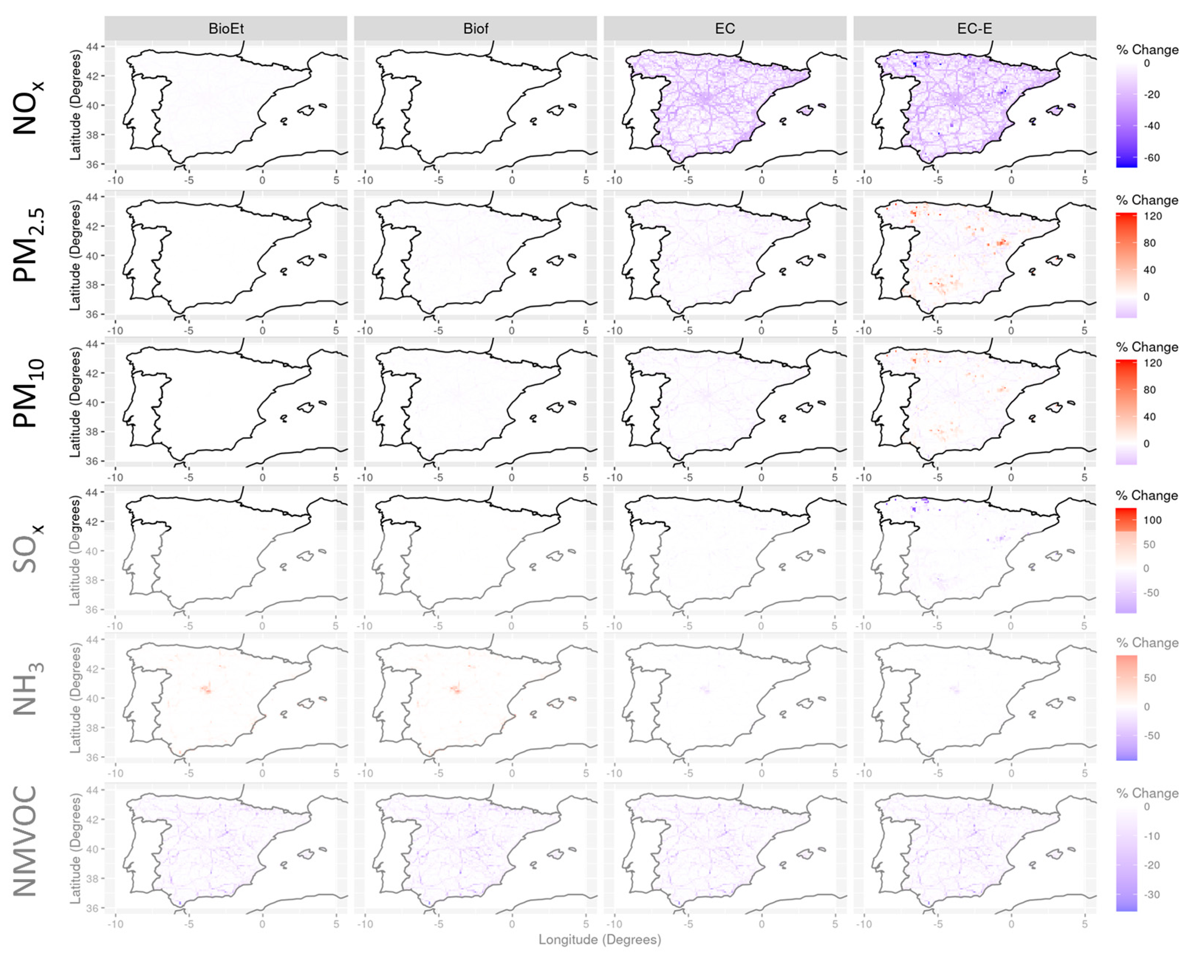
3.1. Air Quality Results
3.2. Avoided Mortality
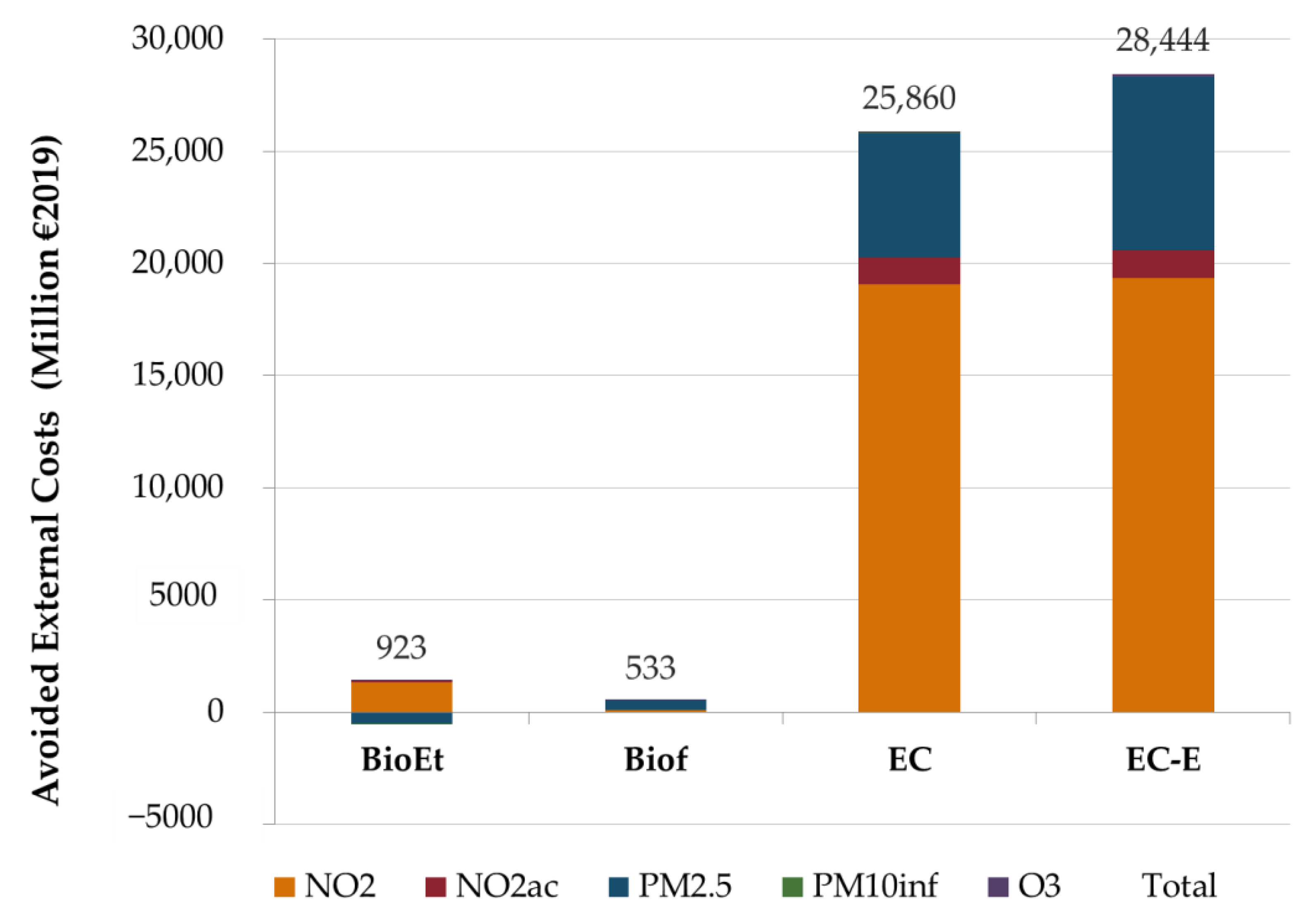
3.3. Avoided External Costs of Mortality Due to Air Pollution
4. Discussion
5. Conclusions
Author Contributions
Funding
Acknowledgments
Conflicts of Interest
Appendix A

| Fuel Use (Kt Oil Equivalent) | No. of Vehicles | Average Travel Distance (km yr−1) | |
|---|---|---|---|
| All road transport | |||
| Total | 28,408.9 | 30,841 197.0 | |
| Cars | |||
| Diesel | 10,840.0 | 13,611,088 | 16,522 |
| Biodiesel | 489.0 | ||
| Petrol | 3641.8 | 7,452,327 | 8696 |
| Bioethanol | 102.3 | 209,239 | 8696 |
| LPG | 47.2 | 44,872 | 16,522 |
| Electric | 1.4 | 12,170 | 9566 |
| CNG | 265.3 | 158,796 | 16,522 |
| Total | 15,387.0 | 21,488,491 | |
| Lorries | |||
| Diesel | 7399.2 | 267,515 | 89,742 |
| Biodiesel | 320.9 | ||
| Petrol ‡ | 32.0 | 2038 | 44,871 |
| Bioethanol | 0.9 | 57 | 44,871 |
| Total | 7753.1 | 269,611 | |
| Vans | |||
| Diesel | 2830.3 | 3,411,130 | 12,671 |
| Biodiesel | 133.1 | ||
| Petrol | 202.1 | 310,804 | 8448 |
| Bioethanol | 5.3 | 8120 | 8448 |
| LPG * | 415.2 | 594,849 | 12,671 |
| CNG # | 11.3 | 6956 | 12,671 |
| Electric | 1.4 | 4 986 | 8448 |
| Total | 3598.6 | 4,336,844 | |
| Urban and regional buses | |||
| Diesel | 912.7 | 55,045 | 6335 |
| Biodiesel | |||
| Petrol | 40.4 | 6335 | |
| Bioethanol | |||
| CNG | 11.3 | 619 | 6335 |
| Electric | 0.9 | 123 | 6335 |
| Total | 965.2 | 55,787 | |
| Motorcycles and small electric vehicles | |||
| Diesel † | 6.5 | 54,474 | 48,562 |
| Biodiesel | 0.3 | ||
| Petrol | 678.6 | 4,493,535 | 19,425 |
| Bioethanol | 19.1 | 126,449 | 19,425 |
| Electric | 0.5 | 16,005 | 48,562 |
| Total | 705.0 | 4,690,464 |
| Scenario | NH3 | NMVOC | NOx | PM2.5 | PM10 | SOx | |
|---|---|---|---|---|---|---|---|
| SNAP 1 (Combustion in the production and transformation of energy) | Baseline 2017 | 1317 | 6324 | 100,744 | 4940 | 6485 | 90,372 |
| EC-E | 1317 | 5565 | 33,246 | 11,412 | 12,633 | 6326 | |
| SNAP 7 (Road transport) | Baseline 2017 | 2439 | 22,354 | 244,713 | 10,009 | 13,999 | 394 |
| BioEt | 7536 | 12,295 | 239,819 | 9909 | 13,860 | 450 | |
| Biof | 7536 | 11,401 | 244,713 | 8808 | 12,319 | 446 | |
| EC and EC-E | 683 | 11,758 | 167,629 | 6729 | 9411 | 188 | |
| Total anthropogenic emissions | Baseline 2017 | 518,192 | 618,717 | 739,031 | 112,771 | 180,240 | 220,275 |
| BioEt | 523,290 | 608,658 | 734,136 | 112,684 | 180,101 | 220,330 | |
| Biof | 523,290 | 607,764 | 739,031 | 111,720 | 178,560 | 220,326 | |
| EC | 516,437 | 608,121 | 661,946 | 109,491 | 175,653 | 220,068 | |
| EC-E | 516,437 | 607,362 | 594,447 | 115,963 | 181,802 | 136,023 |
| Scenario | NH3 | NMVOC | NOx | PM2.5 | PM10 | SOx | |
|---|---|---|---|---|---|---|---|
| SNAP 1 (Combustion in the production and transformation of energy) | EC-E | −− | −12% | −67% | +131% | +95% | −93% |
| SNAP 7 (Road transport) | BioEt | +209% | −45% | −2% | −1% | −1% | +14% |
| Biof | +209% | −49% | −− | −12% | −12% | +13% | |
| EC and EC-E | −72% | −47% | −31% | −33% | −33% | −52% | |
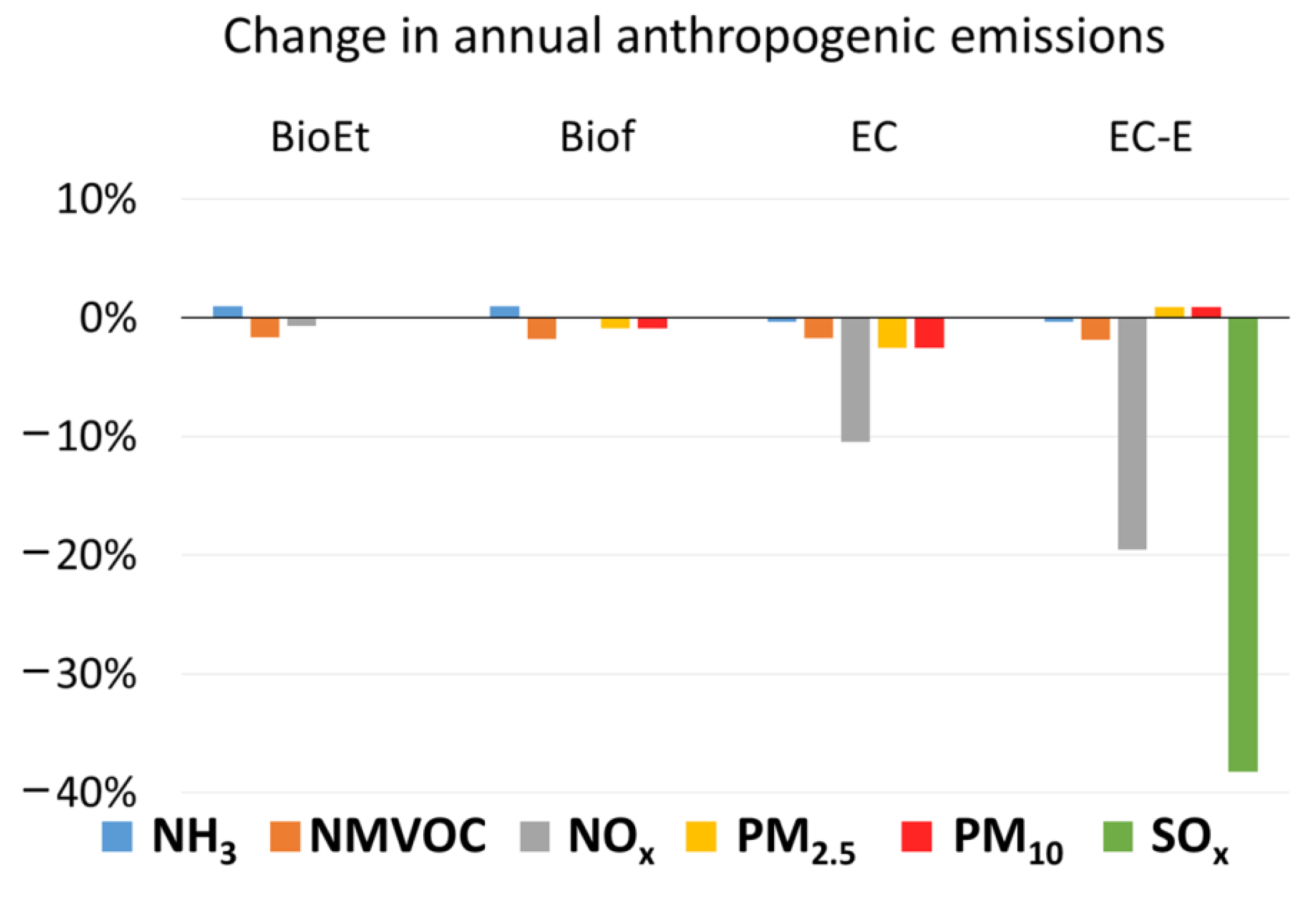
| Total anthropogenic emissions | BioEt | +1% | −2% | −1% | −0.1% | −0.1% | +0.03% |
| Biof | +1% | −2% | −− | −0.9% | −0.9% | +0.02% | |
| EC | −− | −2% | −10% | −3% | −3% | −0.09% | |
| EC-E | −− | −2% | −20% | +3% | +1% | −38% |

| Scenario | Descriptive | Population | Pollution | Mortality | |||||||
|---|---|---|---|---|---|---|---|---|---|---|---|
| All Ages | NO2 Annual Mean | PM2.5 Annual Mean | PM10 Annual Mean | SOMO35 (O3) | NO2 | NO2ac | PM2.5 | PM10 | O3 | ||
| Inhabitants | (µg·m−3) | (µg·m−3) | (µg·m−3) | (ppb·Days) | Premature Deaths (>30 Years) | Premature Deaths | Premature Deaths | Premature Deaths | Premature Infant Deaths | ||
| REF | Mean | 1977.34 | 1.59 | 2.06 | 3.85 | 1802.67 | 0.62 | 0.00 | 1.43 | 0.00 | 0.13 |
| Max | 1,237,053.16 | 46.18 | 19.38 | 36.02 | 14,110.00 | 1388.55 | 3.72 | 1019.18 | 1.26 | 64.83 | |
| Min | 0.00 | 0.00 | 0.00 | 0.00 | 0.00 | 0.00 | 0.00 | 0.00 | 0.00 | 0.00 | |
| BioEt | Mean | 2105.28 | 1.58 | 2.06 | 3.85 | 1799.19 | 0.60 | 0.00 | 1.44 | 0.00 | 0.12 |
| Max | 1,341,460.00 | 45.96 | 19.37 | 36.04 | 14,100.00 | 1373.09 | 3.68 | 1031.38 | 1.26 | 64.75 | |
| Min | 0.00 | 0.00 | 0.00 | 0.00 | 0.00 | 0.00 | 0.00 | 0.00 | 0.00 | 0.00 | |
| Biof | Mean | 2105.28 | 1.60 | 2.05 | 3.84 | 1800.82 | 0.62 | 0.00 | 1.42 | 0.00 | 0.12 |
| Max | 1,341,460.00 | 46.16 | 19.33 | 35.82 | 14,097.44 | 1387.45 | 3.72 | 1008.19 | 1.25 | 64.57 | |
| Min | 0.00 | 0.00 | 0.00 | 0.00 | 0.00 | 0.00 | 0.00 | 0.00 | 0.00 | 0.00 | |
| EC | Mean | 2105.28 | 1.39 | 1.98 | 3.75 | 1771.36 | 0.37 | 0.00 | 1.36 | 0.00 | 0.12 |
| Max | 1,341,460.00 | 43.90 | 19.04 | 35.03 | 14,044.77 | 1144.96 | 3.07 | 933.74 | 1.20 | 67.14 | |
| Min | 0.00 | 0.00 | 0.00 | 0.00 | 0.00 | 0.00 | 0.00 | 0.00 | 0.00 | 0.00 | |
| EC-E | Mean | 2105.28 | 1.36 | 1.90 | 3.63 | 1753.95 | 0.37 | 0.00 | 1.33 | 0.00 | 0.12 |
| Max | 1,341,460.00 | 43.81 | 18.13 | 34.88 | 13,966.01 | 1137.78 | 3.07 | 927.63 | 1.19 | 66.66 | |
| Min | 0.00 | 0.00 | 0.00 | 0.00 | 0.00 | 0.00 | 0.00 | 0.00 | 0.00 | 0.00 | |
References
- European Environment Agency. Transport. Available online: https://www.eea.europa.eu/themes/transport/ (accessed on 21 July 2021).
- Mcadam, K.; Aubin, P.L. Effective Interventions to Mitigate Adverse Human Health Effects from Transportation-Related Air and Noise Pollution A Rapid Review. Available online: https://www.peelregion.ca/health/library/pdf/Rapid-Review-TRAP%20Mitigation.pdf (accessed on 21 July 2021).
- MITECO. Plan Nacional Integrado de Energía y Clima 2021–2030. Available online: https://www.miteco.gob.es/images/es/pnieccompleto_tcm30-508410.pdf (accessed on 20 October 2021).
- MITERD. I Programa Nacional de Control de la Contaminación Atmosférica. Available online: https://www.miteco.gob.es/es/calidad-y-evaluacion-ambiental/temas/atmosfera-y-calidad-del-aire/primerpncca_2019_tcm30-502010.pdf (accessed on 21 July 2021).
- OECD. The Economic Consequences of Outdoor Air Pollution; OECD Publishing: Paris, France, 2016. [Google Scholar]
- Hunt, A.; Ferguson, J.; Hurley, F.; Searl, A. Social Costs of Morbidity Impacts of Air Pollution; OECD Publishing: Paris, France, 2016. [Google Scholar]
- OCDE. The Cost of Air Pollution; OECD Publishing: Paris, France, 2014. [Google Scholar]
- Korzhenevych, A.; Dehnen, N.; Bröcker, J.; Holtkamp, M.; Meier, H.; Gibson, G.; Varma, A.; Cox, V. Update of the Handbook on External Costs of Transport; Final Report Ricardo-AEA/R/ ED57769; Ricardo-AEA: London, UK, 2014. [Google Scholar]
- Im, U.; Brandt, J.; Geels, C.; Hansen, K.M.; Christensen, J.H.; Andersen, M.S.; Solazzo, E.; Kioutsioukis, I.; Alyuz, U.; Balzarini, A.; et al. Assessment and economic valuation of air pollution impacts on human health over Europe and the United States as calculated by a multi-model ensemble in the framework of AQMEII3. Atmos. Chem. Phys. 2018, 18, 5967–5989. [Google Scholar] [CrossRef]
- Román-Collado, R.; Jiménez de Reyna, J. The economic benefits of fulfilling the World Health Organization’s limits for particulates: A case study in Algeciras Bay (Spain). J. Air Waste Manag. Assoc. 2019, 69, 438–449. [Google Scholar] [CrossRef]
- Stern, N. The economics of climate change. In Proceedings of the American Economic Review, New Orleans, LA, USA, 4–6 January 2008; Volume 98, pp. 1–37. [Google Scholar]
- Sanderson, B.M.; O’Neill, B.C. Assessing the costs of historical inaction on climate change. Sci. Rep. 2020, 10, 1–12. [Google Scholar] [CrossRef] [PubMed]
- MCKinsey&Company. Pathways to a Low-Carbon Economy: We Consider Alternative History Scenarios in Which Explicit Climate Mitigation Begins before the Present Day, Estimating the Total Costs to Date of Delayed Action. Considering a 2(1.5) Degree Celsius Stabilization Target. Available online: https://www.cbd.int/financial/doc/Pathwaystoalowcarboneconomy.pdf (accessed on 21 July 2021).
- Edenhofer, O.; Sokona, Y.; Minx, J.C.; Farahani, E.; Kadner, S.; Seyboth, K.; Adler, A.; Baum, I.; Brunner, S.; Kriemann, B.; et al. AR5 Climate Change 2014: Mitigation of Climate Change; Cambridge University Press: New York, NY, USA, 2014. [Google Scholar]
- Sampedro, J.; Smith, S.J.; Arto, I.; González-Eguino, M.; Markandya, A.; Mulvaney, K.M.; Pizarro-Irizar, C.; Van Dingenen, R. Health co-benefits and mitigation costs as per the Paris Agreement under different technological pathways for energy supply. Environ. Int. 2020, 136, 105513. [Google Scholar] [CrossRef]
- Holland, M.R. The Co-Benefits of Different Ambition Levels for Greenhouse Gas Abatement in the EU by 2020. Available online: https://docplayer.net/176646461-The-co-benefits-to-health-of-a-strong-eu-climate-change-policy.html (accessed on 21 July 2021).
- Karlsson, M.; Alfredsson, E.; Westling, N. Climate policy co-benefits: A review. Clim. Policy 2020, 20, 292–316. [Google Scholar] [CrossRef]
- Vandyck, T.; Keramidas, K.; Kitous, A.; Spadaro, J.V.; Van Dingenen, R.; Holland, M.; Saveyn, B. Air quality co-benefits for human health and agriculture counterbalance costs to meet Paris Agreement pledges. Nat. Commun. 2018, 9, 1–11. [Google Scholar] [CrossRef] [PubMed]
- Scovronick, N.; Budolfson, M.; Dennig, F.; Errickson, F.; Fleurbaey, M.; Peng, W.; Socolow, R.H.; Spears, D.; Wagner, F. The impact of human health co-benefits on evaluations of global climate policy. Nat. Commun. 2019, 10, 1–12. [Google Scholar] [CrossRef] [PubMed]
- Xie, Y.; Dai, H.; Xu, X.; Fujimori, S.; Hasegawa, T.; Yi, K.; Masui, T.; Kurata, G. Co-benefits of climate mitigation on air quality and human health in Asian countries. Environ. Int. 2018, 119, 309–318. [Google Scholar] [CrossRef] [PubMed]
- Markandya, A.; Sampedro, J.; Smith, S.; Van Dingenen, R.; Pizarro-Irizar, C.; Arto, I. Health co-benefits from air pollution and mitigation costs of the Paris Agreement: A modelling study. Lancet. Planet. Health 2018, 2, e126–e133. [Google Scholar] [CrossRef]
- Pascal, M.; Corso, M.; Chanel, O.; Declercq, C.; Badaloni, C.; Cesaroni, G.; Henschel, S.; Meister, K.; Haluza, D.; Martin-Olmedo, P.; et al. Assessing the public health impacts of urban air pollution in 25 European cities: Results of the Aphekom project. Sci. Total Environ. 2013, 449, 390–400. [Google Scholar] [CrossRef] [PubMed]
- Izquierdo, R.; García Dos Santos, S.; Borge, R.; Paz, D.; de la Sarigiannis, D.; Gotti, A.; Boldo, E. Health impact assessment by the implementation of Madrid City air-quality plan in 2020. Environ. Res. 2020, 183, 109021. [Google Scholar] [CrossRef]
- Bell, M.L.; Davis, D.L.; Gouveia, N.; Borja-Aburto, V.H.; Cifuentes, L.A. The avoidable health effects of air pollution in three Latin American cities: Santiago, São Paulo, and Mexico City. Environ. Res. 2006, 100, 431–440. [Google Scholar] [CrossRef]
- CE Delft. Health Costs of Air Pollution in European Cities and the Linkage with Transport; CE Delft: Delft, The Netherlands, 2020. [Google Scholar]
- Hamilton, I.; Kennard, H.; McGushin, A.; Höglund-Isaksson, L.; Kiesewetter, G.; Lott, M.; Milner, J.; Purohit, P.; Rafaj, P.; Sharma, R.; et al. The public health implications of the Paris Agreement: A modelling study. Lancet Planet. Health 2021, 5, e74–e83. [Google Scholar] [CrossRef]
- Gallagher, C.L.; Holloway, T. Integrating Air Quality and Public Health Benefits in U.S. Decarbonization Strategies. Front. Public Health 2020, 8, 520. [Google Scholar] [CrossRef]
- Jiang, P.; Chen, Y.; Geng, Y.; Dong, W.; Xue, B.; Xu, B.; Li, W. Analysis of the co-benefits of climate change mitigation and air pollution reduction in China. J. Clean. Prod. 2013, 58, 130–137. [Google Scholar] [CrossRef]
- Kim, S.E.; Xie, Y.; Dai, H.; Fujimori, S.; Hijioka, Y.; Honda, Y.; Hashizume, M.; Masui, T.; Hasegawa, T.; Xu, X.; et al. Air quality co-benefits from climate mitigation for human health in South Korea. Environ. Int. 2020, 136, 105507. [Google Scholar] [CrossRef]
- Peng, W.; Dai, H.; Guo, H.; Purohit, P.; Urpelainen, J.; Wagner, F.; Wu, Y.; Zhang, H. The Critical Role of Policy Enforcement in Achieving Health, Air Quality, and Climate Benefits from India’s Clean Electricity Transition. Environ. Sci. Technol. 2020, 54, 11720–11731. [Google Scholar] [CrossRef]
- Thambiran, T.; Diab, R.D. Air quality and climate change co-benefits for the industrial sector in Durban, South Africa. Energy Policy 2011, 39, 6658–6666. [Google Scholar] [CrossRef][Green Version]
- Mittal, S.; Hanaoka, T.; Shukla, P.R.; Masui, T. Air pollution co-benefits of low carbon policies in road transport: A sub-national assessment for India. Environ. Res. Lett. 2015, 10, 085006. [Google Scholar] [CrossRef]
- Xia, T.; Nitschke, M.; Zhang, Y.; Shah, P.; Crabb, S.; Hansen, A. Traffic-related air pollution and health co-benefits of alternative transport in Adelaide, South Australia. Environ. Int. 2015, 74, 281–290. [Google Scholar] [CrossRef]
- Sarigiannis, D.A.; Kontoroupis, P.; Nikolaki, S.; Gotti, A.; Chapizanis, D.; Karakitsios, S. Benefits on public health from transport-related greenhouse gas mitigation policies in Southeastern European cities. Sci. Total Environ. 2017, 579, 1427–1438. [Google Scholar] [CrossRef]
- ITF/OCDE. Transport Climate Action Directory|Internatiopnal Transport Forum. Available online: https://www.itf-oecd.org/tcad (accessed on 26 July 2021).
- Vivanco, M.G.; Garrido, J.L.; Martín, F.; Theobald, M.R.; Gil, V.; Santiago, J.-L.; Lechón, Y.; Gamarra, A.R.; Sánchez, E.; Alberto, A.; et al. Assessment of the effects of the spanish national air pollution control programme on air quality. Atmosphere 2021, 12, 158. [Google Scholar] [CrossRef]
- Gamarra, A.R.; Lechón, Y.; Vivanco, M.G.; Garrido, J.L.; Martín, F.; Sánchez, E.; Theobald, M.R.; Gil, V.; Santiago, J.L. Benefit Analysis of the 1st Spanish Air Pollution Control Programme on Health Impacts and Associated Externalities. Atmosphere 2020, 12, 32. [Google Scholar] [CrossRef]
- European Union. Directive (EU) 2018/2001 of the European Parliement and of the Council of 11 December 2018 on the Promotion of the Use of Energy from Renewable Sources. Available online: https://eur-lex.europa.eu/eli/dir/2018/2001/oj (accessed on 21 July 2021).
- European Union. Proposal for a firective of the European Parliament and of the Council Amending Directive (EU) 2018/2001 of the European Parliament and of the Council, Regulation (EU) 2018/1999 of the European Parliament and of the Council and Directive 98/70/EC of the European Parliament and of the Council as Regards the Promotion of Energy from Renewable Sources COM/2021/557 Final; European Parliament and of the Council: Brussels, Belgium, 2021. [Google Scholar]
- Alalwan, H.A.; Alminshid, A.H.; Aljaafari, H.A.S. Promising evolution of biofuel generations. Subject review. Renew. Energy Focus 2019, 28, 127–139. [Google Scholar] [CrossRef]
- Ministerio para la Transición Ecológica y el Reto Demográfico. Real Decreto 205/2021, de 30 de Marzo, por el que se modifica el Real Decreto 1085/2015, de 4 de Diciembre, de Fomento de los Biocarburantes, y se Regulan los Objetivos de venta o Consumo de Biocarburantes para los años 2021 y 2022. Available online: https://www.boe.es/diario_boe/txt.php?id=BOE-A-2021-5034 (accessed on 21 July 2021).
- EMEP. 1.A.1 Energy industries. In EMEP/EEA Air Pollutant Emission Inventory Guidebook 2019. Available online: https://www.eea.europa.eu/publications/emep-eea-guidebook-2019 (accessed on 21 July 2021).
- EUSTAT Definition. SNAP Nomenclature. Available online: https://en.eustat.eus/documentos/elem_13173/definicion.html (accessed on 23 August 2021).
- Timmers, V.R.J.H.; Achten, P.A.J. Non-exhaust PM emissions from electric vehicles. Atmos. Environ. 2016, 134, 10–17. [Google Scholar] [CrossRef]
- Ministerio para la Transición Ecológica y el Reto Demográfico. Libro de la Energía en España 2018; Ministerio para la Transición Ecológica y el Reto Demográfico: Madrid, Spain, 2018. [Google Scholar]
- Menut, L.; Bessagnet, B.; Khvorostyanov, D.; Beekmann, M.; Blond, N.; Colette, A.; Coll, I.; Curci, G.; Foret, G.; Hodzic, A.; et al. Chimere 2013: A model for regional atmospheric composition modelling. Geosci. Model Dev. 2013, 6, 981–1028. [Google Scholar] [CrossRef]
- Pirovano, G.; Balzarini, A.; Bessagnet, B.; Emery, C.; Kallos, G.; Meleux, F.; Mitsakou, C.; Nopmongcol, U.; Riva, G.M.; Yarwood, G. Investigating impacts of chemistry and transport model formulation on model performance at European scale. Atmos. Environ. 2012, 53, 93–109. [Google Scholar] [CrossRef]
- Vivanco, M.G.; Palomino, I.; Vautard, R.; Bessagnet, B.; Martín, F.; Menut, L.; Jiménez, S. Multi-year assessment of photochemical air quality simulation over Spain. Environ. Model. Softw. 2009, 24, 63–73. [Google Scholar] [CrossRef]
- Vivanco, M.G.; Palomino, I.; Martín, F.; Palacios, M.; Jorba, O.; Jiménez, P.; Baldasano, J.M.; Azula, O. An evaluation of the performance of the Chimere model over spain using meteorology from MM5 and WRF models. In Proceedings of the Lecture Notes in Computer Science (Including Subseries Lecture Notes in Artificial Intelligence and Lecture Notes in Bioinformatics), Seoul, Korea, 29 June–2 July 2009; Springer: Berlin/Heidelberg, Germany, 2009; Volume 5592 LNCS, pp. 107–117. [Google Scholar]
- Vivanco, M.G.; Correa, M.; Azula, O.; Palomino, I.; Martín, F. Influence of model resolution on ozone predictions over Madrid Area (Spain). In Proceedings of the Lecture Notes in Computer Science (Including Subseries Lecture Notes in Artificial Intelligence and Lecture Notes in Bioinformatics), Perugia, Italy, 30 June–3 July 2008; Springer: Berlin/Heidelberg, Germany, 2008; Volume 5072 LNCS, pp. 165–178. [Google Scholar]
- Bessagnet, B.; Pirovano, G.; Mircea, M.; Cuvelier, C.; Aulinger, A.; Calori, G.; Ciarelli, G.; Manders, A.; Stern, R.; Tsyro, S.; et al. Presentation of the EURODELTA III intercomparison exercise–evaluation of the chemistry transport models’ performance on criteria pollutants and joint analysis with meteorology. Atmos. Chem. Phys. 2016, 16, 12667–12701. [Google Scholar] [CrossRef]
- European Environment Agengy. SOMO35—European Environment Agency. Available online: https://www.eea.europa.eu/help/glossary/eea-glossary/somo35 (accessed on 23 September 2020).
- Holland, M. Implementation of the HRAPIE Recommendations for European Air Pollution CBA Work; International Institute for Applied Systems Analysis: Laxenburg, Austria, 2014. [Google Scholar]
- Soares, J.; Horálek, J.; González, A.; Ortiz Guerreiro, C.; Gsella, A. Health Risk Assessment of Air Pollution in Europe Methodology Description and 2017 Results–Eionet Report–ETC/ATNI 2019/13; European Enviroment Agency: Luxembourg, 2019.
- WHO. Health Risks of Air Pollution in Europe–HRAPIE Project, Recommendations for Concentration–Response Functions for Cost–Benefit Analysis of Particulate Matter, Ozone and Nitrogen Dioxide; WHO: Copenhaga, Denmark, 2013. [Google Scholar]
- WHO. Review of Evidence on Health Aspects of Air Pollution-REVIHAAP Project Technical Report; WHO: Copenhaga, Denmark, 2013. [Google Scholar]
- Hoek, G.; Krishnan, R.M.; Beelen, R.; Peters, A.; Ostro, B.; Brunekreef, B.; Kaufman, J.D. Long-term air pollution exposure and cardio-respiratory mortality: A review. Environ. Health A Glob. Access Sci. Source 2013, 12, 43. [Google Scholar] [CrossRef]
- Samoli, E.; Aga, E.; Touloumi, G.; Nisiotis, K.; Forsberg, B.; Lefranc, A.; Pekkanen, J.; Wojtyniak, B.; Schindler, C.; Niclu, E.; et al. Short-term effects of nitrogen dioxide on mortality: An analysis within the APHEA project. Eur. Respir. J. 2006, 27, 1129–1137. [Google Scholar] [CrossRef]
- Katsouyanni, K.; Samet, J.M.; Ross Anderson, H.; Atkinson, R.; Le Tertre, A.; Medina, S.; Samoli, E.; Touloumi, G.; Burnett, R.T.; Krewski, D.; et al. Air Pollution and Health: A European and North American Approach (APHENA); Health Effects Institute: Boston, MA, USA, 2009. [Google Scholar]
- Gryparis, A.; Forsberg, B.; Katsouyanni, K.; Analitis, A.; Touloumi, G.; Schwartz, J.; Samoli, E.; Medina, S.; Anderson, H.R.; Niciu, E.M.; et al. Acute Effects of Ozone on Mortality from the “Air Pollution and Health: A European Approach” project. Am. J. Respir. Crit. Care Med. 2004, 170, 1080–1087. [Google Scholar] [CrossRef]
- Woodruff, T.J.; Grillo, J.; Schoendorf, K.C. The relationship between selected causes of postneonatal infant mortality and particulate air pollution in the United States. Environ. Health Perspect. 1997, 105, 608–612. [Google Scholar] [CrossRef]
- IGN Centro Nacional de Información Geográfica. (CNIG)–Centro de Descargas del CNIG. Available online: http://centrodedescargas.cnig.es/CentroDescargas/catalogo.do?Serie=CAANE (accessed on 28 September 2020).
- Instituto National de Estadistica. Demografía y Población: Cifras de Población y Censos Demográficos, Proyecciones de Población, Resultados. Available online: https://www.ine.es/dyngs/INEbase/es/operacion.htm?c=Estadistica_C&cid=1254736176953&menu=resultados&idp=1254735572981 (accessed on 28 September 2020).
- European Union. Statistical Regions in the European Union and Partner Countries; European Union: Bruxelles, Belgium, 2020. [Google Scholar]
- Schucht, S.; Colette, A.; Rao, S.; Holland, M.; Schöpp, W.; Kolp, P.; Klimont, Z.; Bessagnet, B.; Szopa, S.; Vautard, R.; et al. Moving towards ambitious climate policies: Monetised health benefits from improved air quality could offset mitigation costs in Europe. Environ. Sci. Policy 2015, 50, 252–269. [Google Scholar] [CrossRef]
- Science Communication Unit, University of the West of England. Science for Environment Policy. What Are the Health Costs of Environmental Pollution? Science Communication Unit, University of the West of England: Bristol, UK, 2018. [Google Scholar]
- Yin, H.; Brauer, M.; Zhang, J.; Cai, W.; Navrud, S.; Burnett, R.; Howard, C.; Deng, Z.; Kammen, D.; Schellnhuber, H.J.; et al. Global Economic Cost of Deaths Attributable to Ambient Air Pollution: Disproportionate Burden on the Ageing Population. medRxiv 2020, 2020.04.28.20083576. [Google Scholar] [CrossRef]
- Viscusi, W.K. Best Estimate Selection Bias in the Value of a Statistical Life. J. Benefit-Cost Anal. 2018, 9, 285–304. [Google Scholar] [CrossRef]
- Viscusi, W.K.; Masterman, C.J. Income Elasticities and Global Values of a Statistical Life. J. Benefit Cost Anal 2017, 8, 226–250. [Google Scholar] [CrossRef]
- OECD. Mortality Risk Valuation in Environment, Health and Transport Policies; Organisation for Economic Cooperation and Development (OECD): Paris, France, 2012; Volume 9789264130. [Google Scholar]
- Roy, R.; Braathen, N.A. The Rising Cost of Ambient Air Pollution thus far in the 21st Century: Results from the BRIICS and the OECD Countries; OECD: Paris, France, 2017. [Google Scholar]
- INE. Cálculo de variaciones del Indice de Precios de Consumo. Available online: https://www.ine.es/varipc/verVariaciones.do?idmesini=1&anyoini=2005&idmesfin=1&anyofin=2019&ntipo=1&enviar=Calcular (accessed on 28 September 2020).
- OECD. Recommended Value of a Statistical Life Numbers for Policy Analysis. In Mortality Risk Valuation in Environment, Health and Transport Policies; OECD Publishing: Paris, France, 2012; pp. 125–136. [Google Scholar]
- CNMC. Dirección de Energía. In Estadística de Biocarburantes. Available online: https://www.cnmc.es/estadistica/estadistica-de-biocarburantes (accessed on 23 September 2020).
- Smeets, E.W.M.; Bouwman, A.F.; Stehfest, E.; van Vuuren, P.; Posthuma, A. Contribution of N2O to the greenhouse gas balance of first-generation biofuels. Glob. Chang. Biol. 2009, 15, 1–23. [Google Scholar] [CrossRef]
- Prussi, M.; Yug, M.; Padella, M.; Edwards, R.; Lonza, L.; De Prada, L. JEC Well-to-Tank Report v5: Annexes Well-to-Wheels Analysis of Future Automotive Fuels and Powertrains in the European Context; Publications Office of the European Union: Luxembourg, 2020. [Google Scholar]
- Prussi, M.; Yugo, M.; De Prada, L.; Padella, M.; Edwards, J.E.C. Well-To-Wheels Report v5; Publications Office of the European Union: Luxembourg, 2020. [Google Scholar] [CrossRef]
- Wernet, G.; Steubing, B.; Reinhard, J.; Bauer, C.; Moreno-Ruiz, E. The ecoinvent database version 3 (part II): Analyzing LCA results and comparison to version 2. Int. J. Life Cycle Assess. 2016, 21, 1269–1281. [Google Scholar] [CrossRef]
- Wernet, G.; Bauer, C.; Steubing, B.; Reinhard, J.; Moreno-Ruiz, E.; Weidema, B. The ecoinvent database version 3 (part I): Overview and methodology. Int. J. Life Cycle Assess. 2016, 21, 1218–1230. [Google Scholar] [CrossRef]
- EMEP/EEA. 1.A.3.b.i-iv Road Transport 2019. In EMEP/EEA Air Pollutant Emission Inventory Guidebook 2019–Update Oct. 2020; European Enviroment Agency: Luxembourg, 2020; Volume 1, p. 1. ISBN 9788578110796. [Google Scholar]
- Lechón, Y.; Cabal, H.; de la Rúa, C.; Lago, C.; Izquierdo, L.; Sáez, R.M.; San Miguel, M.F. Análisis de Ciclo de Vida de Combustibles Alternativos para el Transporte. Fase II. Análisis de Ciclo de Vida Comparativo del Biodiésel y del Diésel; Centro de Publicaciones Secretaría General Técnica, Ministerio de Medio Ambiente: Madrid, Spain, 2006. [Google Scholar]
- Lechón, Y.; Cabal, H.; de la Rúa, C.; Lago, C.; Izquierdo, L.; Sáez, R.M.; San Miguel, M.F. Análisis de Ciclo de Vida de Combustibles Alternativos para el Transporte. Fase I. Análisis de Ciclo de Vida comparativo del etanol de cereales y de la gasolina. Energía y cambio climático; Centro de Publicaciones Secretaría General Técnica, Ministerio de Medio Ambiente: Madrid, Spain, 2005; ISBN 84-8320-312-X. [Google Scholar]
- European Commission. CASES (Cost Assessment of Sustainable Energy System), D.02.2–External Costs, Euro/ton Values; European Commision: Brussels, Belgium, 2008. [Google Scholar]
- Thompson, T.M.; Saari, R.K.; Selin, N.E. Air quality resolution for health impact assessment: Influence of regional characteristics. Atmos. Chem. Phys. 2014, 14, 969–978. [Google Scholar] [CrossRef]
- Gariazzo, C.; Carlino, G.; Silibello, C.; Tinarelli, G.; Renzi, M.; Finardi, S.; Pepe, N.; Barbero, D.; Radice, P.; Marinaccio, A.; et al. Impact of different exposure models and spatial resolution on the long-term effects of air pollution. Environ. Res. 2021, 192, 110351. [Google Scholar] [CrossRef]
- de Ridder, K.; Viaene, P.; van de Vel, K. The impact of model resolution on simulated ambient air quality and associated human exposure. Atmósfera 2014, 27, 403–410. [Google Scholar] [CrossRef]
- Paolella, D.A.; Tessum, C.W.; Adams, P.J.; Apte, J.S.; Chambliss, S.; Hill, J.; Muller, N.Z.; Marshall, J.D. Effect of Model Spatial Resolution on Estimates of Fine Particulate Matter Exposure and Exposure Disparities in the United States. Environ. Sci. Technol. Lett. 2018, 5, 436–441. [Google Scholar] [CrossRef]
- Jiang, X.; Yoo, E.-h. The importance of spatial resolutions of Community Multiscale Air Quality (CMAQ) models on health impact assessment. Sci. Total Environ. 2018, 627, 1528–1543. [Google Scholar] [CrossRef]


| Scenario | Description of Measures | |
|---|---|---|
| Biofuels | BioEt | Renovation of petrol passenger fleet (cars and motorcycles) to flexible–fuel vehicles and the use of E85 petrol (85% bioethanol/15% petrol mixture) by the year 2030. Other petrol vehicles: increase bioethanol content from E5 (5%) to E10 (10%). |
| Biof | Increased biofuel use by two combined measures:
| |
| Electric car | EC | Promotion of electromobility: Current fleet of passenger cars (except hybrids) substituted by electric cars. The scenario does not include the additional electricity generation |
| EC-E | Promotion of electromobility: Current fleet of passenger cars (except hybrids) replaced by electric cars. The scenario includes the additional electricity generation, considering the share of technologies in the power mix for 2030 (considered in NECP) and the change in the absolute production by renewables and fossil technologies. |
| No. Vehicles in 2017 | % Vehicles in 2017 | Number of Vehicles Substituted by Electric Cars in NIECP for 2030 | Number of Vehicles Substituted by Electric Cars in the EC Scenarios | Annual Distance (km/car/year) | Annual Additional EV Car Use (vkm/year) | |
|---|---|---|---|---|---|---|
| Diesel | 13,611,088 | 63.38% | 3,168,859 | 10,442,229 | 16,522 | 1.72 × 10¹¹ |
| Biodiesel | 0 | 0.00% | 0 | 0 | 0 | 0 |
| Petrol | 7,452,327 | 34.70% | 1,735,010 | 5,717,317 | 8696 | 49,717,787,295 |
| Bioethanol | 209,239 | 0.97% | 48,714 | 160,525 | 8696 | 1,395,926,413 |
| LPGs | 44,872 | 0.21% | 10,447 | 34,425 | 16,522 | 568,772,254 |
| CNG | 158,796 | 0.74% | 36,970 | 121,826 | 16,522 | 2,012,808,855 |
| EV/hybrid | 12,170 | 0.06% | 0 | 0 | 9566 | |
| Total | 21,488,491 | 100% | 5,000,000 | 16,476,321 | 2.26 × 10¹¹ |
| Pollutant and Metric | Range of Concentration | Health Outcome (Impact/Population Group) | Type † | RR (95% CI) per 10 μg/m3 | Source |
|---|---|---|---|---|---|
| NO2, annual mean | >20 μg/m3 | Long-term Mortality, all (natural) causes, age over 30 years | B* | 1.055 (1.031–1.080) | [57] |
| NO2, annual mean | All | Acute Mortality, all (natural) causes, all ages | A* | 1.0027 (1.0016–1.0038) | [58] |
| O3, SOMO35 | >35 ppb (>70 µg/m3) | Mortality, all (natural) causes, all ages | A* | 1.0029 (1.0014–1.0043) | [59,60] |
| PM2.5, annual mean | All | Mortality, all (natural) causes, age over 30 years, expressed as Y | A* | 1.062 (1.040–1.083) | [57] |
| PM10, annual mean | All | Post-neonatal infant mortality, (age 1–12 months), all (natural) causes | B* | 1.04 (1.02, 1.07) | [61] |
| Pollutants | Health Outcome | Value of VSL or Premature Death in Spain (€2019/Unit) | Source |
|---|---|---|---|
| NO2, O3, PM | Mortality (VSL) | 3,998,266.36 | Calculated, OECD [71] |
| PM10 | Infant mortality | 6,747,300.00 | OECD [73], Average of High and Low Values |
| BioEt | Biof | EC | EC-E | |
|---|---|---|---|---|
| Unit | Avoided premature deaths (number) | |||
| NO2 | 331 (323–339) | 18 (17–18) | 4771 (4663–4884) | 4839 (4729–4954) |
| NO2ac | 19 (19–19) | 1 (1–1) | 299 (299–300) | 313 (313–314) |
| PM2.5 | −123 (−144–−120) | 110 (107–703) | 1387 (1358–1414) | 1931 (1891–1969) |
| PM10inf | −0.1 (−0.45–−0.08) | 0.14 (0.14–0.67) | 1.14 (1.11–1.17) | 1.5 (1–2) |
| O3 | 5 (5–5) | 5 (5–5) | 8 (8–8) | 28 (28–28) |
| Total | 231 (219–227) | 133 (130–728) | 6467 (6329–6607) | 7113 (6963–7266) |
| BioEt | Biof | ECA | ECB | |
|---|---|---|---|---|
| Unit | Million €2019 | |||
| NO2 | 1323 | 71 | 19,077 | 19,347 |
| NO2ac | 75 | 2 | 1197 | 1252 |
| PM2.5 | −493 | 439 | 5546 | 7722 |
| PM10inf | −1 | 1 | 8 | 10 |
| O3 | 19 | 20 | 32 | 113 |
| Total | 923 | 533 | 25,860 | 28,444 |
| % Reduction | BioEt | Biof | EC | EC-A |
|---|---|---|---|---|
| Reference scenario with Pop. Proj. year 2030 | 0.52% | 0.30% | 14.45% | 15.90% |
| Reference scenario with Pop. 2017 | 7.93% | 8.2% | 7.19% | 8.76% |
Publisher’s Note: MDPI stays neutral with regard to jurisdictional claims in published maps and institutional affiliations. |
© 2021 by the authors. Licensee MDPI, Basel, Switzerland. This article is an open access article distributed under the terms and conditions of the Creative Commons Attribution (CC BY) license (https://creativecommons.org/licenses/by/4.0/).
Share and Cite
Gamarra, A.R.; Lechón, Y.; Vivanco, M.G.; Theobald, M.R.; Lago, C.; Sánchez, E.; Santiago, J.L.; Garrido, J.L.; Martín, F.; Gil, V.; et al. Avoided Mortality Associated with Improved Air Quality from an Increase in Renewable Energy in the Spanish Transport Sector: Use of Biofuels and the Adoption of the Electric Car. Atmosphere 2021, 12, 1603. https://doi.org/10.3390/atmos12121603
Gamarra AR, Lechón Y, Vivanco MG, Theobald MR, Lago C, Sánchez E, Santiago JL, Garrido JL, Martín F, Gil V, et al. Avoided Mortality Associated with Improved Air Quality from an Increase in Renewable Energy in the Spanish Transport Sector: Use of Biofuels and the Adoption of the Electric Car. Atmosphere. 2021; 12(12):1603. https://doi.org/10.3390/atmos12121603
Chicago/Turabian StyleGamarra, Ana R., Yolanda Lechón, Marta G. Vivanco, Mark Richard Theobald, Carmen Lago, Eugenio Sánchez, José Luis Santiago, Juan Luis Garrido, Fernando Martín, Victoria Gil, and et al. 2021. "Avoided Mortality Associated with Improved Air Quality from an Increase in Renewable Energy in the Spanish Transport Sector: Use of Biofuels and the Adoption of the Electric Car" Atmosphere 12, no. 12: 1603. https://doi.org/10.3390/atmos12121603
APA StyleGamarra, A. R., Lechón, Y., Vivanco, M. G., Theobald, M. R., Lago, C., Sánchez, E., Santiago, J. L., Garrido, J. L., Martín, F., Gil, V., & Rodríguez-Sánchez, A. (2021). Avoided Mortality Associated with Improved Air Quality from an Increase in Renewable Energy in the Spanish Transport Sector: Use of Biofuels and the Adoption of the Electric Car. Atmosphere, 12(12), 1603. https://doi.org/10.3390/atmos12121603