Green’s Function for Static Klein–Gordon Equation Stated on a Rectangular Region and Its Application in Meteorology Data Assimilation

Abstract

The meteorology data assimilation applications often encounter variational problems with unknown weights, where the corresponding Euler equation is an elliptic partial differential equation. This research focused on retrieving the weights in remote sensing data assimilation by means of the computer-friendly form of the Green’s function obtained by eigenfunction expansion for the boundary value problem of the static Klein–Gordon equation on a rectangular region. With the help of the proposed retrieving method, the assimilation problem of estimating regional precipitation with weather radar and rain-gauge is solved in the Green’s function method. Results show that high accuracy of the proposed method makes it a good candidate for data assimilation problems in operational use.

1. Introduction

In modern numerical weather prediction, data assimilation is an effective method to improve data accuracy by fusing datasets with different precisions. Data assimilation applications often encounter variational problems, where the corresponding Euler equation is an elliptic partial differential equation (PDE), usually a static Klein–Gordon equation (SKGE). In applications, there are two obstacles: unknown boundary conditions, and unknown weights. Such problems of retrieving the unknown boundary condition and weights are generally known as inverse problems. Most previous research on these problems has concentrated on approximating parameter estimation [1,2,3,4,5] to some extent. Wei, et al. (1998, 2003) calculated the weights with the matrix theory and the finite difference method of partial differential equation [6,7].

In solving elliptic equations by Green’s functions, Melnikov (2011) constructed the corresponding Green’s functions for the SKGE of several unbounded domains into convergent series, which were more suitable for the numerical implementation [8]. Using Fourier transformation, Aseeri et al. (2015) solved the cubic Klein-Gordon equation and examined strong scaling of the code [9]. Vibrating systems examples were described by Klein–Gordon equation and the correspondence between the classical and quantum settings of this equation was discussed in [10]. Muravey (2015) provided explicit formulas for the Green’s functions of an elliptic PDE in an infinite strip and a half-plane [11]. However, due to convergence of series, the explicit Green’s function on a rectangular region remains unsolved. Cheng, et al. (2017) found the representation in double series of Green’s function for SKGE on a rectangular region. Although it is uniformly convergent, the huge amount of computing complexity along with the double series hinders the practical application [12].

Needless to say, the retrieval of the unknown weights of an elliptic PDE requires the explicit solution based on the Green’s function, which is in the form of an infinite series. In fact, retrieving the weights is more difficult than retrieving the unknown boundary condition, because the weights appear in the expression of Green’s function. Considering the approximation calculation, the infinite series of the Green’s function must be acquired in a computer-friendly form. This is the motivation of our research.

This current work obtains a new series representation of the Green’s function for the SKGE using eigenfunction expansion. The Green’s function is decomposed into a singular component and a regular component. The singular component, with a logarithmic singularity, is expressed as an explicit elementary function, which is computer-friendly for Green’s function application. The regular component is expressed as an infinite series. The uniform convergence of this infinite series is investigated. With help of the computer-friendly form Green’s function, the weights are calculated by comparing the observations in the interior region with the formula solution of Green’s function in the corresponding positions. Real precipitation data assimilation results show that Green’s function method is a good candidate for data assimilation problems in operational use.

2. The Data Assimilation and Its Variational Problem

In weather prediction areas, a particular physical parameter $u_R$ is provided from remote observation. The corresponding physical quantity $\tilde{u}$ retrieved from $u_R$ according to the empirical formula is usually with large error. Some high-precision observation $u_G$ in the same area can be used to improve the estimation accuracy, but the number of high-precision observations is limited. More reasonable constraints are also needed to improve the estimation accuracy. According to the smoothness and the dependence on the observation, an unknown function $u\left(x,y\right)$ is built to satisfy the following functional extremum problem

$$\underset{\mathsf{\Omega }}{\overset{ }{{\displaystyle \iint }}}\left[{\left(\frac{\partial u}{\partial x}\right)}^2+{\left(\frac{\partial u}{\partial y}\right)}^2+{\mu }_R{\left(u-u_R\right)}^2+{\mu }_G{\left(u-u_G\right)}^2\right]dxdy=\min$$

(1)

where $\mathsf{\Omega }$ stands for a special field, ${\mu }_R\ge 0,{\mu }_G\ge 0$ are weights corresponding to different error items. In addition, the values of $u\left(x,y\right)$ on the boundary $\mathsf{\Gamma }$ of area $\mathsf{\Omega }$ are given by

$$u\left(x,y\right){|}_{\mathsf{\Gamma }}=\varphi \left(x,y\right)$$

(2)

For this functional extremum problem with the boundary constraint, the corresponding Euler’s equation is presented as follows [13,14]:

$$\frac{{\partial }^{2}u}{\partial x^2}+\frac{{\partial }^{2}u}{\partial y^2}-\mu u=\widehat{u} ,$$

(3)

where $\widehat{u}={\mu }_R{u}_R+{\mu }_G{u}_G$, $\mu ={\mu }_R+{\mu }_G$. This is a typical Dirichlet problem for an elliptic equation stated on a special region. Theoretically, the elliptic equation can be solved by the Green’s function. However, as mentioned before, the weights are usually unknown in real data assimilation problem.

The Green’s function of a PDE depends on not only the form of the equation but also the boundary condition. It is important to find an explicit solution of the Green’s function [12]. In order to get an analytical expression of the corresponding Green’s function, we consider the special situation of a rectangular area. The solution of Equation (3) has area of

$$\mathsf{\Omega }=\left\{\left(x,y\right)|0\le x\le a,0\le y\le b\right\}.$$

For simplicity of discussion, in this paragraph, let $k^2=\mu ,f=\widehat{u}$, we discuss the Klein–Gordon equation as follows.

$$\{\begin{array}{c}{\nabla }^{2}u-k^{2}u=f \\ u{|}_{\mathsf{\Gamma }}=\varphi \end{array}$$

(4)

As Hilbert has shown, a boundary problem is solvable if a generalized Green’s function is introduced. Therefore, we should find the corresponding Green’s function—i.e.,$G\left(x,y;\xi ,\eta \right)$—which satisfies [13]

$$\{\begin{array}{l}{\nabla }^{2}G-k^{2}G=\delta \left(x-\xi \right)\delta \left(y-\eta \right) \\ G{|}_{\mathsf{\Gamma }}=0 \end{array}$$

(5)

for any point $\left(\xi ,\eta \right)$ in domain $\mathsf{\Omega }$. Here, $\delta$ is a Dirac function.

On the other hand, if $u\left(x,y\right),G\left(x,y;\xi ,\eta \right)\in C^2\left(\mathsf{\Omega }\right)$, from the Green’s function, we have

$${{\displaystyle \iint }}_{\mathsf{\Omega }}^{ }\left[u{\nabla }^{2}G-G{\nabla }^{2}u\right]dxdy={{\displaystyle \int }}_{\mathsf{\Gamma }}^{ }\left(u\frac{\partial G}{\partial \stackrel{\rightharpoonup }{n}}-G\frac{\partial u}{\partial \stackrel{\rightharpoonup }{n}}\right)ds.$$

(6)

where $\stackrel{\rightharpoonup }{n}$ is normal vector of the boundary $\mathsf{\Gamma }$. Let u satisfy Equation (4), substituting u into Equation (6) gives

$${{\displaystyle \iint }}_{\mathsf{\Omega }}^{ }\left[u{\nabla }^{2}G-G\left(k^{2}u+f\right)\right]dxdy={{\displaystyle \int }}_{\mathsf{\Gamma }}^{ }\left(u\frac{\partial G}{\partial \stackrel{\rightharpoonup }{n}}-G\frac{\partial u}{\partial \stackrel{\rightharpoonup }{n}}\right)ds.$$

Then, for a generalized Green’s function satisfying Equation (5), the above equation can be simplified as

$$\begin{array}{c}{{\displaystyle \iint }}_{\mathsf{\Omega }}^{ }\left[u\left({\nabla }^{2}G-k^{2}G\right)-Gf\right]dxdy={{\displaystyle \iint }}_{\mathsf{\Omega }}^{ }u\delta \left(x-\xi ,y-\eta \right)dxdy-{{\displaystyle \iint }}_{\mathsf{\Omega }}^{ }Gfdxdy\\ ={{\displaystyle \int }}_{\mathsf{\Gamma }}^{ }\left(u\frac{\partial G}{\partial \stackrel{\rightharpoonup }{n}}-G\frac{\partial u}{\partial \stackrel{\rightharpoonup }{n}}\right)ds.\end{array}$$

The solution of Equation (4) therefore becomes

$$u\left(\xi ,\eta \right)={{\displaystyle \iint }}_{\mathsf{\Omega }}^{ }G\left(x,y;\xi ,\eta \right)f\left(x,y\right)dxdy+{{\displaystyle \int }}_{\mathsf{\Gamma }}^{ }\varphi \left(x,y\right)\frac{\partial G\left(x,y;\xi ,\eta \right)}{\partial \stackrel{\rightharpoonup }{n}}ds$$

(7)

The next key problem is to get the solution of Equation (5), the generalized Green’s function $G\left(x,y;\xi ,\eta \right)$.

It is well known that non-homogeneous boundary conditions can be transformed into homogeneous boundary conditions. For simplicity, we assume that $\varphi \left(x,y\right)=0$ here. Then we get

$$u\left(\xi ,\eta \right)={{\displaystyle \iint }}_{\mathsf{\Omega }}^{ }G\left(x,y;\xi ,\eta \right)f\left(x,y\right)dxdy={{\displaystyle \int }}_0^b{{\displaystyle \int }}_0^{a}G\left(x,y;\xi ,\eta \right)f\left(x,y\right)dxdy$$

(8)

where the Green’s function $G\left(x,y;\xi ,\eta \right)$, according to the Appendix A, is defined by

$$\left(x,y;\xi ,\eta \right)=\frac{2}{b}{\displaystyle \sum }_{n=1}^{\infty }{g}_n\left(x,\xi \right)\sin vy\sin v\eta ,v=\frac{n\pi }{b}$$

(9)

The coefficients $g_n\left(x,\xi \right)$ for $x<\xi$ are of the form

$$\begin{array}{c}{g}_n\left(x,\xi \right)=\frac{1}{4h\sin \mathrm{h}ha}[\exp \left(h\left(x-\xi -a\right)\right)-\exp \left(h\left(x+\xi -a\right)\right)\\ +\exp \left(-h\left(x-\xi -a\right)\right)-\exp \left(-h\left(x+\xi -a\right)\right)]\end{array}$$

(10)

where $h=\sqrt{{\upsilon }^2+k^2}$. Substituting (9), (10) into (8) yields

$$\begin{array}{cc}u\left(\xi ,\eta \right)=\hfill & \frac{2}{b}{{\displaystyle \int }}_0^b{{\displaystyle \int }}_0^{\xi }{\displaystyle {\displaystyle \sum }_{n=1}^{\infty }}\frac{\sinh h\left(\xi -a\right)\sinh hx}{h\sinh ha}\sin \upsilon y\sin \upsilon \eta f\left(x,y\right)dxdy\hfill \\ & +\frac{2}{b}{{\displaystyle \int }}_0^b{{\displaystyle \int }}_{\xi }^a{\displaystyle {\displaystyle \sum }_{n=1}^{\infty }}\frac{\sinh h\xi \sinh h\left(x-a\right)}{h\sinh ha}\sin \upsilon y\sin \upsilon \eta f\left(x,y\right)dxdy\hfill \end{array}$$

(11)

where $f={\mu }_R{u}_R+{\mu }_G{u}_G$.

3. Retrieving the Weights by Formal Solution

Obviously, formal solution expression (8) contains unknown parameters,${\mu }_R,{\mu }_G$. The mechanism for retrieving is to minimize the error between the observations and the analytical solution in the observation points. It is well known that the analytical solution can be obtained if the Green’s function of the PDE is known. In the previous section, a computer-friendly representation of the Green’s function is developed, the approximation calculation of analytical solution can be implemented by directly truncating the infinite series.

As precipitation data $u_G$ measured by rain gauge is more accurate, we try to select the weights that satisfy

$$J\left({\mu }_R,{\mu }_G\right)={\displaystyle \sum }_{\left(\xi ,\eta \right)\in {\mathsf{\Omega }}_G}^{ }{\left(u\left(\xi ,\eta \right)-u_G\left(\xi ,\eta \right)\right)}^2=min.$$

(12)

where ${\mathsf{\Omega }}_G$ represents the rain gauge point set. According to the knowledge of calculus, we compute the partial derivatives as follows

$$\begin{array}{l}\frac{\partial J}{\partial {\mu }_R}=2{\displaystyle {\displaystyle \sum }_{\left(\xi ,\eta \right)\in {\mathsf{\Omega }}_G}^{ }}\left(u\left(\xi ,\eta \right)-u_G(\xi ,\eta \right))\frac{\partial u\left(\xi ,\eta \right)}{\partial {\mu }_R}\\ =2{\displaystyle {\displaystyle \sum }_{\left(\xi ,\eta \right)\in {\mathsf{\Omega }}_G}^{ }}\left(u-u_G\right)[{{\displaystyle \int }}_0^a{{\displaystyle \int }}_0^{b}G\left(x,y;\xi ,\eta \right)\frac{\partial f}{\partial {\mu }_R}dxdy\\ +{{\displaystyle \int }}_0^a{{\displaystyle \int }}_0^b\frac{\partial G\left(x,y;\xi ,\eta \right)}{\partial {\mu }_R}fdxdy],\\ \frac{\partial J}{\partial {\mu }_G}=2{\displaystyle {\displaystyle \sum }_{\left(\xi ,\eta \right)\in {\mathsf{\Omega }}_G}^{ }}\left(u\left(\xi ,\eta \right)-u_G(\xi ,\eta \right))\frac{\partial u\left(\xi ,\eta \right)}{\partial {\mu }_G}\\ =2{\displaystyle {\displaystyle \sum }_{\left(\xi ,\eta \right)\in {\mathsf{\Omega }}_G}^{ }}\left(u-u_G\right)[{{\displaystyle \int }}_0^a{{\displaystyle \int }}_0^{b}G\left(x,y;\xi ,\eta \right)\frac{\partial f}{\partial {\mu }_G}dxdy\\ +{{\displaystyle \int }}_0^a{{\displaystyle \int }}_0^b\frac{\partial G\left(x,y;\xi ,\eta \right)}{\partial {\mu }_G}fdxdy]\end{array}$$

where $\frac{\partial f}{\partial {\mu }_R}=u_R$, $\frac{\partial f}{\partial {\mu }_G}=u_G$,

$$\begin{array}{c}\frac{\partial G\left(x,y;\xi ,\eta \right)}{\partial {\mu }_R}=\frac{2}{b}{\displaystyle \sum }\frac{\partial g_n\left(x,\xi \right)}{\partial {\mu }_R}\sin \nu y\sin \nu \eta ,\\ \frac{\partial G\left(x,y;\xi ,\eta \right)}{\partial {\mu }_G}=\frac{2}{b}{\displaystyle \sum }\frac{\partial g_n\left(x,\xi \right)}{\partial {\mu }_G}\sin \nu y\sin \nu \eta \end{array}$$

with

$$\begin{array}{ll}\frac{\partial g_n\left(x,\xi \right)}{\partial {\mu }_R}& =\frac{\partial g_n\left(x,\xi \right)}{\partial h}\frac{\partial h}{\partial {\mu }_R}=\frac{\partial g_n\left(x,\xi \right)}{\partial h}\frac{1}{2h},\\ \frac{\partial g_n\left(x,\xi \right)}{\partial {\mu }_G}& =\frac{\partial g_n\left(x,\xi \right)}{\partial h}\frac{\partial h}{\partial {\mu }_G}=\frac{\partial g_n\left(x,\xi \right)}{\partial h}\frac{1}{2h},\\ \frac{\partial g_n\left(x,\xi \right)}{\partial h}& =\frac{\partial }{\partial h}\left(\frac{\sinh h\left(\xi -a\right)\sinh hx}{h\sinh ha}\right)\\ & =\frac{[\left(\xi -a\right)\cosh h\left(\xi -a\right)+x\cosh hx]h\sinh ha}{h^2{\sinh }^{2}ha}\\ & -\frac{\left(\sinh ha+h\cosh ha\right)\sinh h\left(\xi -a\right)\sinh hx}{h^2{\sinh }^{2}ha}.\end{array}$$

$$\begin{array}{ll}\frac{\partial g_n\left(x,\xi \right)}{\partial {\mu }_R}& =\frac{\partial g_n\left(x,\xi \right)}{\partial h}\frac{\partial h}{\partial {\mu }_R}=\frac{\partial g_n\left(x,\xi \right)}{\partial h}\frac{1}{2h},\\ \frac{\partial g_n\left(x,\xi \right)}{\partial {\mu }_G}& =\frac{\partial g_n\left(x,\xi \right)}{\partial h}\frac{\partial h}{\partial {\mu }_G}=\frac{\partial g_n\left(x,\xi \right)}{\partial h}\frac{1}{2h},\\ \frac{\partial g_n\left(x,\xi \right)}{\partial h}& =\frac{\partial }{\partial h}\left(\frac{\sinh h\left(\xi -a\right)\sinh hx}{h\sinh ha}\right)\\ & =\frac{[\left(\xi -a\right)\cosh h\left(\xi -a\right)+x\cosh hx]h\sinh ha}{h^2{\sinh }^{2}ha}\\ & -\frac{\left(\sinh ha+h\cosh ha\right)\sinh h\left(\xi -a\right)\sinh hx}{h^2{\sinh }^{2}ha}.\end{array}$$

Finally, the steepest descent algorithm is designed for solving $J\left(\overrightarrow{z}\right)\triangleq J\left({\mu }_R,{\mu }_G\right)=\min$.

Algorithm:

• Step 1. Choose initial point ${\overrightarrow{z}}^{\left(0\right)}=\left({\mu }_R^{\left(0\right)},{\mu }_G^{\left(0\right)}\right)$, l = 0, precise requirement $\epsilon >0$;
• Step 2. Calculate $\nabla J\left({\overrightarrow{z}}^{\left(l\right)}\right)=\left(\frac{\partial J}{\partial {\mu }_R},\frac{\partial J}{\partial {\mu }_G}\right){\overrightarrow{z}}^{\left(l\right)},{\overrightarrow{z}}^{\left(l\right)}=\left({\mu }_R^{\left(l\right)},{\mu }_G^{\left(l\right)}\right)$. If $\parallel \nabla J\left({\overrightarrow{z}}^{\left(l\right)}\right)\parallel <\epsilon$, stop. Otherwise, let ${\overrightarrow{d}}^{\left(l\right)}=-\nabla J\left({\overrightarrow{z}}^{\left(l\right)}\right)$;
• Step 3. Let ${\overrightarrow{z}}^{\left(l+1\right)}={\overrightarrow{z}}^{\left(l\right)}+{\lambda }_l{\overrightarrow{d}}^{\left(l\right)}$, find ${\lambda }_l$ from $J\left({\overrightarrow{z}}^{\left(l+1\right)}\right)=\min$;
• Step 4. Let $l=l+1$, turn to Step 2.

According to the Appendix B, convergence analysis and truncation error analysis, the series representation of Green’s function is uniformly converged, and the calculation of infinite series can be truncated.

4. Numerical Experiments

Simulations are conducted here to find the rate of convergence, and so investigate the performance of the proposed Green’s function in Equation (7). Figure 1 plots $G\left(x,y;\xi ,\eta \right)$ on the rectangular region (0 ≤ x ≤ 80, 0 ≤ y ≤ 60) selected from the radar detection range for $\left(\xi ,\eta \right)$ equals to (40, 30). Note that G equals 0 on the boundaries of the region and tends to −∞ when $\left(x,y\right)$ tends to $\left(\xi ,\eta \right)$. The convergence performance of the Green’s function on many points in the rectangular area is tested to perform the simulation. Results show that all the points converge steadily to their true numerical values after a limited number of iterations. The convergence speed of the Green’s function is much faster when $\left(x,y\right)$ is far from $\left(\xi ,\eta \right)$.

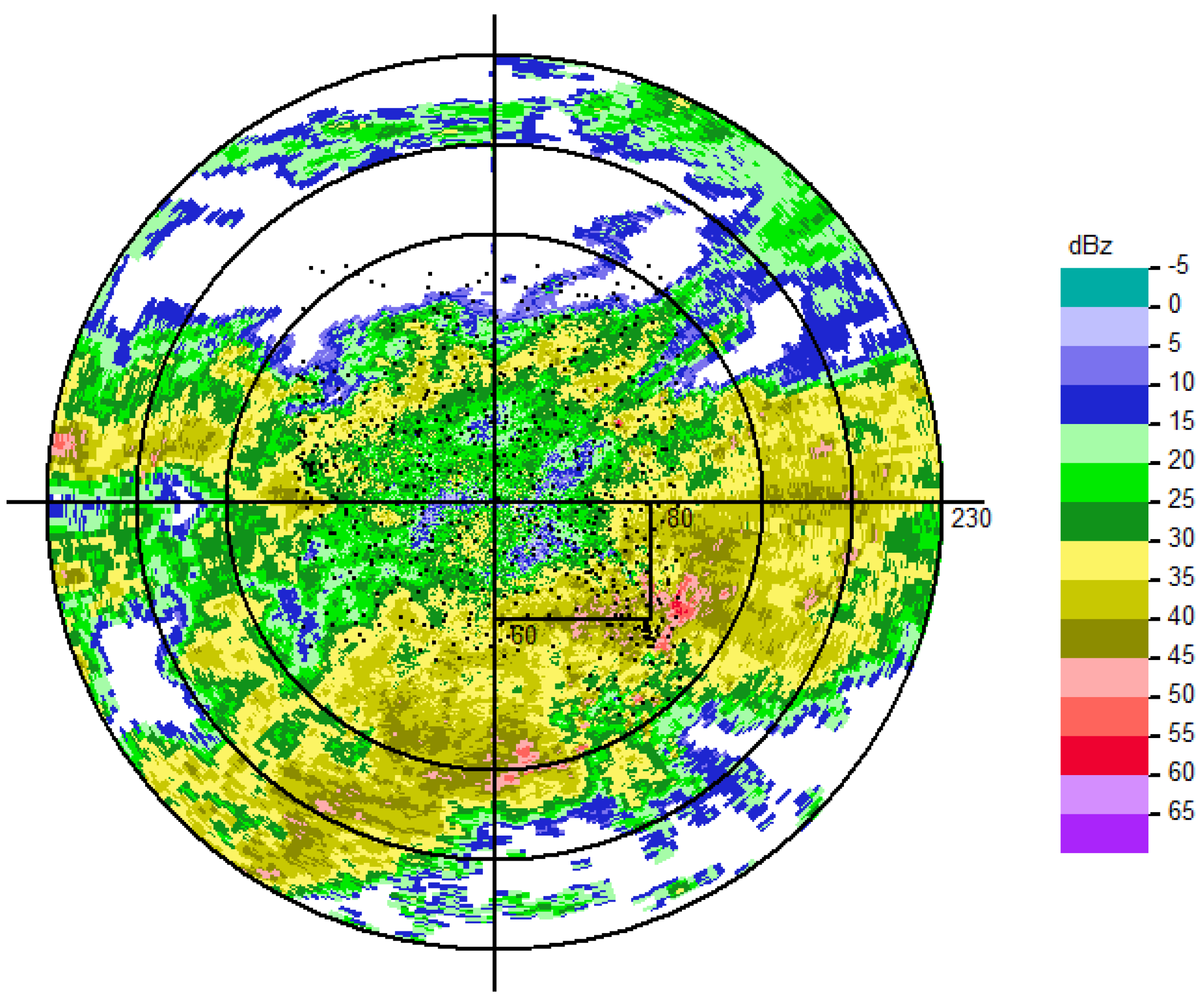
In the following example, the Green’s function method in Equation (8) is used to retrieve the rainfall value at some points in a rectangular area. The results are compared with the values from the Z-I relationship. The observation data are made by Changzhou radar at 18:38 UTC on 11 June 2016 (Figure 2). There are 624 rain gauges in the observation area. In the data assimilation problem, the 624 rain-gauges data are used to correct radar–retrieved rainfall. The optimal estimation weights are ${\mu }_R=12,{\mu }_G=96$.

A rectangular region of 80 × 60 km² (Figure 3) and 103 rain gauges inside it are chosen to perform the Green’s function method. Because it is a rectangular region, using partial derivative to replace directional derivative, we get the curve integral on the four boundaries by difference method. Assuming boundary condition equals the radar observation, rainfall of every rain-gauge point in the rectangular region is obtained by the Green’s function method.

In practical application, if the number of rain gauges is insufficient, virtual observations on positions without rain gauges can be obtained by linear interpolation. In our experiment, there are few rain gauges near the bottom of the rectangular area. At (50, 50), for example, the observed value 0.953 is obtained by interpolation of five nearby observation points (42, 55), (47, 41), (57, 46), (50, 45) and (53, 48), which can be used for subsequent parameter estimation or comparative analysis.

In the calculation, 75 rain gauges are selected to estimate the weights, and the remaining quarter of the rain gauges are used for comparative analysis. The results show that the retrieved values possess better correlation properties of the rain-gauge observations than radar observations (Figure 4). Correlation coefficient has grown from 0.6149 to 0.7844. Most retrieved values of the 103 points are closer to the rain-gauge observations than the values from Z-I relationship of radar and rainfall. Under the condition of optimal weights selection, the rainfall field obtained by variational inversion has higher accuracy. In this case, Z-I relationship is Z = 296 ∗ I^1.24 in which Z is the radar reflectivity, I is the rainfall $u_R$.

Table 1. Interior point values. Pos is interior point coordinates (unit: km). Obs is rain-gauge observation in 10 min (unit: mm). Rad is radar observation on the point (unit: dBz). Rtr is retrieved data by Z-I relationship of radar and rainfall (unit: mm). Joi is the joint value by the Green’s function method (unit: mm).

Pos	(17, 47)	(59, 21)	(62, 58)	(78, 36)	(67, 44)	(50, 28)	(28, 22)	(52, 25)
Obs	1.2	0.7	1.8	2.7	2.3	0.9	0.2	0.6
Rad	30	27	47	35	38	31	11	30
Rtr	1.2322	0.9353	3.2013	1.6780	3.5835	0.9404	0.1644	0.7484
Joi	0.2224	0.1274	5.2259	0.5629	0.9826	0.2678	0.0065	0.2224

shows some of these values.

5. Conclusions

This study solves the data assimilation problems of two kinds of data, $u_R$ and $u_G$, through a variational model. In order to retrieve the weighting parameters ${\mu }_R,{\mu }_G$ from some of the observations in the interior region, the computer-friendly form of the Green’s function is obtained by eigenfunction expansion for the boundary value problem of the static Klein–Gordon equation on a rectangular region. Convergence analysis in Appendix B proves that the series representation of Green’s function is computer-friendly, and can be used to approximate computations by a direct truncation.

The numerical experiment’s result shows that the series representation of Green’s function converges steadily and rapidly. The Green’s function method is used to retrieve the weights and assimilate precipitation data from weather radar and rain-gauges in the experiments. Results show that the Green’s function method is a good candidate for data assimilation problems in operational use.

References

1. Talagrand, O.; Courtier, P. Variational assimilation of meteorological observations with the adjoint vorticity equation. I: Theory. Q. J. R. Meteorol. Soc. 1987, 113, 1311–1328. [Google Scholar] [CrossRef]
2. Al-Jamal, M.F. Numerical Solution of Elliptic Inverse Problems via the Equation Error Method. Ph.D. Thesis, Michigan Technological University, Houghton, MI, USA, 2012. [Google Scholar]
3. Mehraliyev, Y.T.; Kanca, F. An inverse boundary value problem for a second order elliptic equation in a rectangle. Math. Modeling Anal. 2014, 19, 241–256. [Google Scholar] [CrossRef] [Green Version]
4. Mehraliyev, Y.T. On solvability of an inverse boundary value problem for a fourth order elliptic equation. J. Math. Syst. Sci. 2013, 3, 560–566. [Google Scholar]
5. Orlovsky, D.G. Inverse problem for elliptic equation in Banach space with Bitsadze—Samarsky boundary value conditions. J. Inverse ILL-Posed Probl. 2013, 21, 141–157. [Google Scholar] [CrossRef]
6. Ming, W.; Renqing, D.; Wenzhong, G.; Takeda, T. Retrieval Single-Doppler Radar Wind with Variational Assimilation Method—Part I: Objective Selection of Functional Weighting Factors. Adv. Atmos. Sci. 1998, 15, 553–567. [Google Scholar] [CrossRef]
7. Ming, W.; Guo-qing, L.; Cheng-gang, W.; Wen-zhong, G.; Qin, X. Optimal Selection for the Weighted Coefficients of the Constrained Variational Problems. Appl. Math. Mech. 2003, 24, 926–944. [Google Scholar] [CrossRef]
8. Melnikov, Y.A. Construction of Green’s functions for the two-dimensional static Klein-Gordon equation. J. Part. Differ. Equ. 2011, 24, 114–139. [Google Scholar]
9. Aseeri, S.; Batrašev, O.; Icardi, M.; Leu, B.; Liu, A.; Li, N.; Muite, B.K.; Müller, E.; Palen, B.; Quell, M. Solving the Klein-Gordon equation using Fourier spectral methods: A benchmark test for computer performance. In Proceedings of the Symposium on High Performance Computing (HPC’15), Montreal, QC, Canada, 17 June 2015; pp. 182–191. [Google Scholar]
10. Gravel, P.; Cauthier, C. Classical applications of the Klein-Gordon equation. Am. J. Phys. Teach. 2011, 79, 447–453. [Google Scholar] [CrossRef]
11. Muravey, D. The boundary value problem for a static 2D Klein-Gordon equation in the infinite strip and in the half-plane. Mathematics 2015, 40, 205–227. [Google Scholar]
12. Cheng, H.; Mu, X.; Jiang, H.; Liu, G.; Wei, M. Green’s Function for the boundary value problem of thestatic Klein-Gordon equation stated on a rectangular region and its convergence analysis. Bound. Value Probl. 2017, 2017, 72. [Google Scholar] [CrossRef] [Green Version]
13. Courant, R.; Hilbert, D. Methods of Mathematical Physics; Interscience Publishers Inc.: New York, NY, USA, 1953. [Google Scholar]
14. Sasaki, Y.K. Some basic formulisms in numerical variational analysis. Mon. Weather Rev. 1970, 98, 875–883. [Google Scholar] [CrossRef] [Green Version]
Figure 1. Plot of the Green’s function G(x, y; ξ, η) on a rectangular region.
Atmosphere 12 01602 g001
Figure 2. Radar observation and rain-gauge point position.
Atmosphere 12 01602 g002
Figure 3. Rectangular Region (80 × 60 km2).
Atmosphere 12 01602 g003
Figure 4. 10 min rainfall from different methods.
Atmosphere 12 01602 g004