Article

Turbulence of Landward and Seaward Wind during Sea-Breeze Days within the Lower Atmospheric Boundary Layer

1
CNRS, UMR 8187—LOG—Laboratoire d’Océanologie et de Géosciencesm, Université de Lille, Université Littoral Côte d’Opale, F 62930 Wimereux, France
2
EA 4493—LPCA—Laboratoire de Physico-Chimie de l’Atmosphère, Université Littoral Côte d’Opale, F 59140 Dunkerque, France
*
Authors to whom correspondence should be addressed.
Atmosphere 2021, 12(12), 1563; https://doi.org/10.3390/atmos12121563
Submission received: 9 October 2021 / Revised: 20 November 2021 / Accepted: 24 November 2021 / Published: 26 November 2021
(This article belongs to the Special Issue Air-Sea Interaction and Ocean Dynamics)

Abstract

:
Reynolds stress anisotropy is estimated from the stress spheroids, based on 20 Hz ultrasonic anemometer measurements, performed in the coastal area of northern France, over a 1.5-year long period. Size and shape variation (i.e., prolate, oblate, disk, rod, etc.) of stress spheroids are used for the characterization of energy redistribution by turbulent eddies. The sea-breeze (SB) events were identified using a change in wind direction from seaward (SWD) to landward (LWD) during the day time. We found that the LWD wind creates more turbulent anisotropic states than SWD wind. The prolate-shaped stress spheroids correspond to small-scale turbulence observed during LWD wind, while oblate spheroids are found during SWD winds. Moreover, it was found that during LWD winds, large turbulence kinetic energy (TKE) in the flow field produces large stress spheroids. On the contrary, during SWD winds, a smaller level of TKE is responsible for small-size stress spheroid formation. The average volume of the corresponding Reynolds stress spheroids during the LWD is 13% larger than that of during SWD wind.

1. Introduction

Meteorological phenomena (such as sea-breeze and nocturnal low-level jets) affect the air quality within the industrial and urban areas near the shoreline [1,2,3]. During summer, the daytime thermal contrast between lands and sea leads to an air density difference, resulting in the occurrence of sea-breeze (SB). The SB properties are dependent on the topography of the land, atmospheric processes (e.g., the occurrence of clouds and synoptic forcing), and turbulent convection [4,5]. Injection of humid cold air from the maritime boundary layer into the ascending inland air leads to the generation of convective clouds, which can be a cause of strong thunderstorms and convective precipitation [6]. Baker et al. [7] revealed that SB-initiated precipitation in a coastal area affects the surrounding air quality. The vertical circulation within SB, characterized by large up and downward velocities, results in the modulation of air quality and further environmental complications [8]. In addition, SB can enhance the dispersion of pollutants through gravity currents [9].
The numerical study of Briere [10] showed that the interaction between convection and mean shear can alter the turbulence intensity during SB. Later, a field study by Chiba [11] showed transformations in turbulence parameters within the lower atmospheric boundary layer due to SB. Laboratory experiment by Cenedese et al. [12] showed that the generation of turbulence over the land was decreased in the presence of sea-breeze (SB) fronts. Cuxart et al. [13] reported that the turbulence intensity and kinetic energy increased during the initiation of SB, then remained constant till afternoon, and finally decreased at nighttime.
During the last several decades, due to the development of offshore wind farms, SB gained much attention. Steele et al. [14,15] stated that coastal wind turbines produce lower energy before the initiation of SB, and increase energy production during SB. Kumar et al. [16] reported that the energy production is enhanced by 15% during SB days. However, during SB days, the sudden change of wind speed, direction, and turbulence has an adverse effect on wind turbines [17]. Rizza et al. [6] stated that wind shear plays an important role in the occurrence of turbulence in SB. The evolution from the isotropic turbulence to the anisotropic turbulence during SB days can be understood from the Reynolds stress tensor (RST). Therefore, the quantification of turbulence using RST is an efficient tool.
In this study, we suggest a new perception of the turbulence variability during SB days, using the RST anisotropy with the corresponding invariants [18]. In our approach, we use stress tensor separation into isotropic and anisotropic parts. The turbulence momentum and energy transport can be highlighted by the anisotropic part of the RST [19]. Therefore, turbulence anisotropy can be used to describe the turbulence energy transfer and dissipation [20]. The relationship between the dissipation tensor and the RST in axisymmetric turbulence was evaluated by Banerjee et al. [21].
A number of field, laboratory, and numerical studies were focused on characterizing SB [11,12,13]. However, information on the landward wind (LWD) and seaward wind (SWD) variability and turbulence anisotropy during SB days is missing in the literature. In the present study, we focus on assessing the turbulence variability in the atmospheric boundary layer (ABL) during sea-breeze days. This assessment is important for the wind energy production industry as well as for air quality monitoring. We also quantify the turbulence kinetic energy (TKE), rms velocity, TKE dissipation, and length-scales for LWD corresponding to the SB flow and SWD wind. Moreover, we assess the three-dimensional shape of Reynolds stress, which shows the energy distribution and describes its variability. In Section 2, we present the data and the methods used for the analysis; the discussions of the results are presented in Section 3, followed by the conclusion in Section 4.

2. Data and Methods

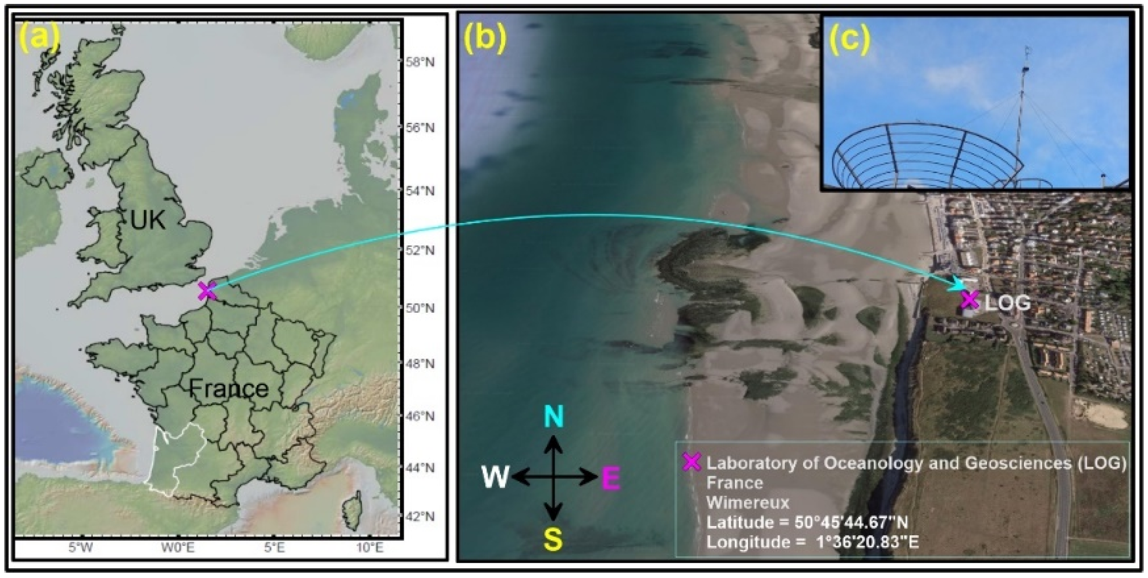
2.1. Study Area, Data Collection and Sea-Breeze Detection

Figure 1a,b shows the map of measurement location in the north of France. A 20 Hz ultrasonic anemometer (shown in Figure 1c) was deployed on the rooftop (15 m above from the ground) of the Laboratory of Oceanology and Geosciences (LOG) site for collecting the wind speed during a 1.5-year period from June 2018 to November 2019 and assessing to the wind variability.
In the present study, a shift in wind direction from offshore to onshore was identified from an alteration of the sign of SB component (SBC) from negative to positive as: S B C = U × sin ( 0 W D ) , where W D is the wind direction and U is the horizontal wind speed [1,22] (zero angle corresponds to the wind direction from the north with positive values measured clockwise). We used a normalized SB component (SBCN = SBC/U) to detect SB days. A negative value of SBCN (~−1) indicates the easterly wind (SWD) and a positive value (~1) matches the westerly wind (LWD). In this study, the sonic measurement of zonal, meridional, and vertical velocity components is defined as ur, vr, and wr, respectively. Note that the positive zonal component represents the wind blowing from the west, the positive meridional component vr characterizes the wind blowing from the south, and the positive vertical component wr matches the wind blowing upward. In order to interpret the fluctuating behavior of the wind in an optimal way, we have adopted a frame of reference using a coordinate system with the x-axis aligned with the mean wind for each averaging period (15 min) [23]. In this case, the horizontal wind is decomposed into the along (streamwise) and cross (transverse) wind components. In this coordinate system, the anisotropy and the structures of turbulence can be properly quantified. The velocity vector projection onto axis in meteorological coordinate frame can modify the shape of turbulence structures. The new coordinate system aligned with the mean flow direction allows to avoid this effect.
Most of the SB days were observed within the summer (May to August). Based on the SBCN calculation, we have selected 49 SB events. Figure 2a provides the wind rose for the period from 1st May to 31st August 2019 and Figure 2b shows all selected SB days. In each wind rose plot, 15 min averaged wind speed and direction were used during a 24 h period (00:00–24:00 UTC). It is clear that wind from the east-south-east (SWD) and west-south-west (LWD) dominated during SB days (Figure 2b).
Figure 2c shows the averaged SBCN (all selected SB days) as a function of time. The SWD wind is predominant during the nighttime (00:00 to 06:30 UTC), while LWD wind blows during the daytime (09:00 to 16:00 UTC). Note that the transition period from SWD to LWD (06:30 to 09:00) is characterized by different turbulence structures due to rapid change in wind speed and direction. In addition, this period is not the same for all SB days. To avoid the effect of turbulence structures from the transition period on the SWD and LWD wind turbulence, we have considered ±30 min tolerance for each SB day. In this study, we did not consider the wind variability during the period from 16:00 up to 20:00 UTC, because it corresponds to a transition period between LWD and SWD wind. Since the SBCN within the period from 20:00 up to 00:00 UTC is not similar to the SWD wind, we did not consider this region as SWD. A rapid change in wind direction, speed, and temperature during the SB days may create a difference in turbulence within the lower troposphere in the coastal regions. In subsequent analysis, turbulence parameters are calculated for all 49 SB days. As such, we have distinguished SWD and LWD during the SB days and performed an estimation of turbulence parameters for these two stages of wind.

2.2. Methodology

The streamwise, transverse, and vertical velocity components (u, v, and w) of the turbulent flow were decomposed into a mean part and fluctuating part as:
u = u ¯ + u ,   v = v ¯ + v ,   w = w ¯ + w ,
where u , v , and   w are three components of the instantaneous velocity vector, u ¯ , v ¯ ,   and   w ¯ are 15 min averaged velocity components, and u , v ,   and   w are the corresponding velocity fluctuations. Many studies have used an averaging time around 15 min to estimate turbulent fluxes [24,25,26]. Indeed, the convective timescale is around 10 or 15 min in the mid-afternoon [27]. Moreover, a 15 min averaging time is a good compromise because it is large enough to ensure that the low-frequency limit of the inertial subrange is well resolved in the FFT (fast Fourier transform), thus allowing the deduction of the dissipation rate [28]. Further, it is short enough to ensure steady state mean meteorological conditions according to Taylor’s hypothesis [25].
The root mean-square velocity (rms) is calculated as:
r m s   v e l o c i t y = 1 3 ( σ u 2 + σ v 2 + σ w 2 ) ,
where σ u ,   σ v , and σ w are the standard deviations of u , v , and w components of wind velocity, respectively. Therefore, u ¯ 2 = σ u 2 ,   v ¯ 2 = σ v 2 and w ¯ 2 = σ w 2 , where overbar denotes 15 min averaged.
The time-averaged Reynolds shear stress components are defined as:
R u v = u v ¯ ;   R u w = u w ¯ ;   R v w = v w ¯ .
The Turbulence Kinetic Energy (TKE) can be written as:
T K E = 3 2 ( r m s   v e l o c i t y ) 2 .
Further, we calculated the fluctuating energy ( E ) as:
E = 1 2 ( u 2 + v 2 + w 2 ) .
The streamwise, transverse, and vertical turbulence kinetic energy flux ( F u , F v and F w ) can be expressed as:
F u = E u ¯ ,   F v = E v ¯   and   F w = E w ¯ .
The TKE dissipation rate (ε) is calculated using velocity spectral density values E u ( f ) in the inertial subrange [29] as:
ε = 2 π U ¯ ( f 5 / 3 E u ( f ) α ) 3 / 2 ,
where U ¯ is the mean wind speed, f is frequency and α is the Kolmogorov constant = 0.52.
The turbulence length-scale (L) is calculated as:
L = T K E 3 / 2   ε .
The Reynolds stress tensor (RST) is a symmetric second-order tensor, given by:
τ = R i j = [   u 2 ¯           u v ¯           u w ¯   v u ¯             v 2 ¯           v w ¯   w u ¯             w v ¯           w 2 ¯ ] .
Any symmetric matrix can be decomposed into isotropic R i j i s o and anisotropic R i j a n i s o parts.
R i j = R i j i s o + R i j a n i s o .
In the case of isotropy, turbulence motions are independent in three-dimensional space domain and Reynolds normal stresses ( u u ¯ = v v ¯ = w w ¯ ) are identical. On the contrary, unequal normal stresses ( u u ¯ v v ¯ w w ¯ ) characterize anisotropic turbulence. The decomposition of RST can be performed as:
R i j i s o = 1 3 Κ 2 δ i j ;   R i j a n i s o = R i j R i j i s o .
Here Κ 2 = 2   T K E and δ i j = { 1 , ( if   i = j ) 0 , ( if   i j )
For further analysis, the anisotropic part is considered in its non-dimensional form
χ i j = R i j a n i s o Κ 2 = R i j Κ 2 δ i j 3 = [   u 2 ¯ Κ 2 1 3           u v ¯ Κ 2         u w ¯   Κ 2   v u ¯ Κ 2           v 2 ¯ Κ 2 1 3         v w ¯ Κ 2   w u ¯   Κ 2           w v ¯ Κ 2         w 2 ¯ Κ 2 1 3 ] .
The anisotropy tensor χ i j is considered to be the fundamental characteristic of the turbulence anisotropy. The anisotropy tensor is nondimensional, has zero traces, and is bounded by 1 3 χ i j 2 3 . It disappears for isotropic cases.
The characteristic equation of χ i j for second-order tensor can be written as:
λ 1 3 I λ 2 3 + I I λ 3 I I I = 0 ,
where, λ 1 ,   λ 2 ,   and   λ 3 are the eigenvalues and the principal invariants, and I , I I ,   and   I I I are defined as [20]:
I = χ i i = 0 ;       I I = χ i j χ j i / 2 ;   I I I = χ i j χ j k χ k i / 3 = | χ i j | .

3. Characteristics of Seaward and Landward Wind Turbulence

3.1. Assessment of TKE and Rms Velocity

In atmosphere, TKE represents the mean kinetic energy of the turbulence per unit mass within wind flow [30]. Figure 3 shows the probability density function (PDF) of the TKE for LWD and SWD wind during SB days. The TKE density for SWD wind (PDF = 1 at TKE = 0.4 m2s−2) is slightly smaller than that for LWD wind (PDF = 0.7 at TKE = 0.8 m2s−2).
From Figure 3 it is clear that the wind energy is larger for LWD compared to SWD wind during SB days. Fluctuations during LWD wind could be increased by the effect of TIBL (Thermal Internal Boundary Layer) whereas, during the SWD, the buoyancy is reduced in the nocturnal boundary layer so that the TKE is low.

3.2. Probability Density of Energy Dissipation Rate and Length-Scale of Turbulent Eddies

The probability density of TKE dissipation rate ε is evaluated using a one-dimensional velocity spectrum method for both LWD and SWD wind during SB days, shown in Figure 4. A peak density (PDF =20) is found at a value of ε = 0.015 m2s−3 for LWD wind, however, the PDF =50 at ε = 0.01 m2s−3 for SWD wind. A large density peak for small value of ε signifies that the TKE dissipation within SWD wind is smaller than LWD wind. This result is coherent since the values of TKE and rms velocity for SWD are also smaller than for LWD wind. A tight correlation of ε with TKE was highlighted by Puhales et al. [31].
The turbulence length-scale (L) which is known as the dissipation length is calculated using the dissipation rate and TKE. Thus, the influence of TKE and ε on L is expected. Figure 5 shows the probability density distribution of length-scale for LWD and SWD winds. Peak values of probability distribution observed at L = 18 m for SWD wind, and L = 25 m for LWD wind are observed. The probability of occurrence of large length-scales for LWD wind is slightly higher than for SWD wind (Figure 5).
Since the measurements were performed not far from the ground (15 m above ground level) there may be some effects of micro-orography on the flow field (e.g., neighboring buildings or large tree) for SWD wind. However, near-ground obstacles faintly affect the upper flow field. Since the study area is on the seashore, there is no existence of a large structure on the seaside but some buildings and elevated topographies are there on the landside. For LWD wind there is no micro-orographic effect. Figure 5 shows small dissipation length-scales for SWD wind. We speculate that the micro-orographic effect can be one of the factors for small values of L. Presence of obstacles within the SWD wind flow field can generate vortex shedding, which can create smaller turbulence eddies. The eddy scales depend of the dimensions of the obstacles.

3.3. Quadrant Analysis of TKE Fluxes

Streamwise ( F u ) and vertical ( F w ) turbulence kinetic energy fluxes are shown jointly in Figure 6a,b and the flux direction is identified using a four-quadrant frame, Q1–Q4. Blue dots located in Q1 show TKE fluxes in the direction opposite to the mean flow direction and upward (OF-UP). TKE fluxes shown in Q2 have direction along the mean flow and upward (AF-UP). Q3 and Q4 quadrants show fluxes along with (AF-DW), opposite (OF-DW) to the mean flow and downward. This analysis helps in understanding the direction of the TKE flux during SB events.
For LWD wind, the maximum probability of TKE flux is observed in the opposite direction of the mean flow and upward, as maximum data are located in Q1 (Figure 6a). However, for SWD wind, the maximum probability of TKE flux is found in Q1 and Q2 (Figure 6b). During SB days, the LWD wind blows along the streamwise direction, but the TKE flux is opposite to the mean flow. We found that this flux causes an increase in TKE dissipation rate (Figure 4 and Figure 6a). On the contrary, during the SWD wind, equal distribution of TKE flux along and opposite the mean flow direction provides a decrease in TKE dissipation rate (Figure 4 and Figure 6b). In addition, large upward TKE flux (PDF peak at F w = 0.1 m3s−3) is observed within LWD wind (Figure 6a). Upward TKE flux within SWD wind is also observed but the value of F w is smaller (PDF peak at F w = 0.025 m3s−3) than that for LWD wind (Figure 6a). The fact that the TKE flux is upward merely says that TKE is being exported from near the surface to higher up.

3.4. Reynolds Stress Anisotropy

States of stress spheroids are shown in Appendix A. For isotropic case the value of ξ and η should be zero. Figure 7 shows the AIM (anisotropy invariant map) in ξη space, computed for LWD and SWD wind during SB days, where ξ and η are modified invariants. No isotropic state is found for both LWD and SWD winds. Axisymmetric expansion and contraction are observed for both LWD and SWD winds which indicates the existence of prolate and oblate stress spheroids (in Figure 7, the right and left cluster of data points, respectively) in the flow field. This map is good for qualitative analysis but it is difficult to distinguish the turbulence states for LWD and SWD winds.
For better quantification of the 3D anisotropic turbulence, an invariant function (ζ = 1 + 27III + 9II) is calculated. This anisotropic invariant function (ζ) provides a perception of the anisotropic stress distribution ranging between two limits: two-component turbulence (ζ = 0) and isotropic turbulence (ζ = 1) [32]. For two component turbulences II = ( 3 I I I + 1 / 9 ) , for prolate spheroids II = 3 ( I I I / 2 ) 2 / 3 , for oblate spheroids I I = 3 ( I I I / 2 ) 2 / 3 , and for isotropic turbulence II = III = 0. Since the absolute value of I I is the same for both prolate and oblate spheroids, it is very difficult to distinguish the particular shape of spheroids using ζ.
For LWD and SWD wind, ζ is calculated and the probability density distribution of ζ is plotted in Figure 8. Maximum probability density of ζ is observed at ζ = 0.88 for SWD and ζ = 0.64 for LWD wind, which signifies that the LWD wind is slightly more anisotropic than SWD wind. The internal boundary layer after the onset of the SB creates an unstable stratification of ABL resulting in an increment of shear stress within the roughness layer (measurement location) [33]. The increment of anisotropy may be due to the increment of shear stress during LWD.
To make a possible connection between the stress spheroid and TKE, the nondimensional degree of anisotropy D a = I I I / 2 ( I I / 3 ) 1.5 is calculated. Liberfigurezon et al. [34] stated that the value of Da typically varies from −1 (along the left side curve of AIM) to 1 (along the right-side curve of AIM).
Figure 9 shows the variability of the TKE as a function of the degree of anisotropy (Da). The maximum TKE is observed at the Da range starting from 0.1 to 0.8 for LWD wind, which signifies that the prolate-shaped stress spheroids have a maximum TKE for LWD wind. After “axisymmetric” expansion, the streamwise component of normal stress is being stretched more than vertical and transverse components. The maximum TKE concentration within prolate-shaped stress spheroids suggests that a TIBL develops during LWD winds limiting the increase of the convective boundary layer top during daytime. Large wind shear during the LWD [1] creates prolate-shaped stress spheroids. However, a large value of TKE is observed at the Da range −0.3 to 0, which signifies that the oblate-shaped stress spheroids contain large TKE within SWD wind. It may be due to the stable stratification of ABL during the nighttime (the wind shear is comparatively low).
To visualize the actual size of stress spheroids, we have introduced the modified AIM map. For better perception, we have modified the coordinates as, x = 100ξ, y = 100η, and z = 50. Note that z (separation distance) is a pseudo number it can be adjusted for distinct visualization, this number does not have any effect on spheroid sizes. In the present study, we have tried different values of z and selected a range z = 1 to 50 for good representation. Each spheroid is estimated using 15 min averaged normal stress. Three normal stress components are used to construct the stress spheroids. Note that all normal stress components are computed from raw sonic data with the x-axis of coordinate system being aligned along the mean flow.
Figure 10 shows the actual size of stress spheroids for LWD and SWD winds during SB days. The prolate and oblate stress spheroids are clearly seen for both LWD and SWD winds. However, the size of spheroids is larger for LWD wind than SWD wind. We found large stress spheroids where energy redistribution is confined within a large volume of spheroid during LWD winds (Figure 10a). On the contrary, during SWD winds, the energy redistribution is limited within a smaller volume of stress spheroid (Figure 10b). The average volume of these spheroid during the LWD is 13% higher than SWD wind.
Figure 6 shows that the magnitude of F u and F v is similar and slightly higher than F w during SWD wind. Therefore, the distribution of TKE fluctuations along the x- and y-axis is equal and higher than that along the z-axis within oblate spheroids (Figure 10b).Magnitudes of F u are large than that of F v and are much larger than that of F w , within these prolate spheroids during LWD winds (Figure 10a). In the atmosphere, the shape of stress spheroids has an influence on pollutant transport and mixing in three dimensions. This can lead to particular pollutant dispersal processes such as the fumigation phenomenon which can be significantly involved in the increase of pollutants’ ground-level concentrations during daytime sea breeze events.

4. Conclusions

Wind measurements by ultrasonic anemometer over 1.5 years in the coastal region are used for assessment of the dynamics of landward (LWD) and seaward (SWD) winds during SB days. The analysis of three-dimensional wind speed revealed a total of 49 SB days during the summertime. High-frequency wind measurements by ultrasonic anemometer showed that the turbulence kinetic energy and rms of velocity are different for LWD and SWD winds during SB days. Large anisotropy in turbulence has been found between two stages of SB days. We show that the turbulence energy distribution is also different for LWD and SWD winds, which may affect the air quality in the coastal region during SB days. In addition, the modulation of turbulence energy distribution, length-scales, dissipation, and anisotropy for LWD and SWD winds during the SB days can have favorable and adverse effects on the wind turbines and on air quality in coastal regions. Analysis conducted in the present study explores these turbulence parameters.
Our analyses revealed significant differences in turbulence characteristics for LWD and SWD winds during SB days are the following:
  • During the SB days the TKE is relatively larger for LWD compared to SWD winds.
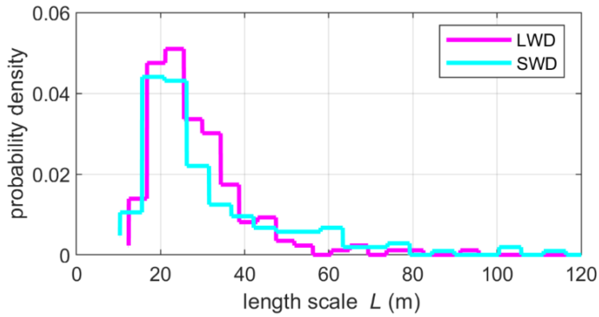
  • The TKE dissipation rate is smaller for SWD wind than for LWD wind, resulting in larger sized (maximum probability of occurrence of L = 25 m) turbulence eddies developing for LWD wind conditions and smaller sizes (maximum probability of occurrence of L = 20 m) for SWD wind conditions.
  • During SB days, the LWD wind blows along the streamwise direction, but the TKE flux is opposite to the mean flow. We found that this flux causes an increase in TKE dissipation rate. On the contrary, during the SWD wind, equal distribution of TKE flux along and opposite the mean flow direction provides a decrease in TKE dissipation rate.
  • The proposed modified AIM performed better to capture the exact size of stress spheroids after axisymmetric expansion and contraction than previous two-dimensional AIM. It is found that LWD wind turbulence is more anisotropic than that of SWD wind. Prolate and oblate stress spheroids are formed due to this anisotropy.
  • Large fluctuations of TKE in the flow field create large stress spheroids where the energy distribution is confined within a large area of prolate spheroids during LWD winds. On the contrary, during SWD winds, small fluctuations of TKE in the flow field give rise to a small oblate stress spheroids with the energy distribution limited to a smaller area of spheroid.
The results on SBCN, large TKE and dissipation rate during LWD wind are in good agreement with Augustin et al. [1]. Note that information on TKE flux and anisotropy during LWD and SWD is new. We found an adverse gradient of wind speed during the transition period between SWD and LWD. This variation in wind speed may change the turbulence structures during the transition period. There is future work to do concerning the transition period, during which the anisotropy and stress spheroid shape could be different than during the SWB and LWB shapes because of the development of the ABL.

Author Contributions

Conceptualization, S.R. and P.A.; methodology, S.R. and P.A.; software, S.R., M.F. and P.A.; validation, S.R., M.F. and P.A.; formal analysis, S.R. and P.A.; investigation, P.A.; resources, P.A. and M.F.; data curation, S.R., P.A. and M.F.; writing—original draft preparation, S.R. and A.S.; writing—review and editing, S.R., A.S., P.A. and M.F.; supervision, A.S. and P.A.; project administration, A.S. and P.A.; funding acquisition, A.S. and P.A. All authors have read and agreed to the published version of the manuscript.

Funding

This project was funded by the Université du Littoral Côte d’Opale, EDF Renouvelables, the Institut de Recherche Pluridisciplinaire en Sciences de l’Environnement (IRePSE) and the Pôle de Recherche Environnement, Milieux Littoraux et Marins (EMLM) of Université du Littoral Côte d’Opale.

Institutional Review Board Statement

Not applicable.

Informed Consent Statement

Not applicable.

Data Availability Statement

Not applicable.

Conflicts of Interest

The authors declare no conflict of interest.

Appendix A

In 3D space, isotropic turbulence can be represented as variable shape stress spheroid. It represents idealized wind equally fluctuating in all directions, without a preferential direction [19]. The basic physics behind isotropic turbulence is that the three-dimensional velocity fluctuations are independent of the axis of rotation. Therefore, it means that all the normal stresses are equal ( τ d 1 = τ d 2 = τ d 3 ), where d1, d2 and d3 are x, y and z direction indicators respectively. The AIM is useful to quantify the development of the Reynolds stress anisotropy in the wind turbulence [18,20]. Since this map was constructed using the actual invariant values (II and III from Equation (14)), the area under the map is very narrow. To improve this situation researchers implemented a new plot with modified invariants ξ (defined as ξ = I I / 2 3 ) and η ( η = I I I / 3 2 )).
In this study, the AIM is constructed with the modified invariants (Figure A1), where the origin (ξ = η = 0) characterizes the three-dimensional (3D) isotropic turbulence ( τ d 1 = τ d 2 = τ d 3 ), at this point the stress ellipsoid has a spherical form [32]. The left vertex of the AIM (Figure A1) having ξ = −1⁄6; η = 1⁄6 matches to the two-component (2D) isotropic (i.e., axisymmetric) turbulence, where z component of the stress vanishes with the remaining two being equal ( ( τ d 1   τ d 2 ) > τ d 3 ). After an axisymmetric contraction, i.e., along the line η = −ξ, it has an oblate shape (left line of AIM shown in Figure 7 and Figure A1) since the z component is lower than x and y components of the normal stress ( ( τ d 1   τ d 2   or   τ d 1   τ d 2 ) > τ d 3 ). After an axisymmetric expansion, i.e., along the line limit η = +ξ, it has a prolate shape (right line of AIM shown in Figure 7 and Figure A1) since the x component of the normal stress is higher than two others ( τ d 1 > ( τ d 2   τ d 3   or   τ d 2   τ d 3 ) ). The one component of turbulence with only one stress component ( τ d 1 > 0 ; ( τ d 2 = τ d 3 = 0 ) ) is at the uppermost right vertex of the triangle with limit ξ = η = 1/3. The non-linear ( η = ( 1 27 + 2 ξ 3 ) 0.5 ) curve connects the left and right vertices, along this curve the stress ellipsoid becomes an elliptic disk.
Figure A1. AIM in ξ, η framework showing all conceivable understanding of turbulence states.
Atmosphere 12 01563 g0a1

References

  1. Augustin, P.; Billet, S.; Crumeyrolle, S.; Deboudt, K.; Dieudonné, E.; Flament, P.; Fourmentin, M.; Guilbaud, S.; Hanoune, B.; Landkocz, Y.; et al. Impact of sea breeze dynamics on atmospheric pollutants and their toxicity in industrial and urban coastal environments. Remote Sens. 2020, 12, 648. [Google Scholar] [CrossRef] [Green Version]
  2. Setyan, A.; Flament, P.; Locoge, N.; Deboudt, K.; Riffault, V.; Alleman, L.Y.; Schoemaecker, C.; Arndt, J.; Augustin, P.; Healy, R.M.; et al. Investigation on the near-field evolution of industrial plumes from metalworking activities. Sci. Total Environ. 2019, 668, 443–456. [Google Scholar] [CrossRef]
  3. Talbot, C.; Augustin, P.; Leroy, C.; Willart, V.; Delbarre, H.; Khomenko, G. Impact of a sea breeze on the boundary-layer dynamics and the atmospheric stratification in a coastal area of the North Sea. Bound. Layer Meteorol. 2007, 125, 133–154. [Google Scholar] [CrossRef]
  4. Crumeyrolle, S.; Augustin, P.; Rivellini, L.H.; Choël, M.; Riffault, V.; Deboudt, K.; Fourmentin, M.; Dieudonné, E.; Delbarre, H.; Derimian, Y.; et al. Aerosol variability induced by atmospheric dynamics in a coastal area of Senegal, North-Western Africa. Atmos. Environ. 2019, 203, 228–241. [Google Scholar] [CrossRef]
  5. Augustin, P.; Delbarre, H.; Lohou, F.; Campistron, B.; Puygrenier, V.; Cachier, H.; Lombardo, T. Investigation of local meteorological events and their relationship with ozone and aerosols during an ESCOMPTE photochemical episode. Ann. Geophys. 2006, 24, 2809–2822. [Google Scholar] [CrossRef] [Green Version]
  6. Rizza, U.; Miglietta, M.M.; Anabor, V.; Degrazia, G.A.; Maldaner, S. Large-eddy simulation of sea breeze at an idealized peninsular site. J. Mar. Syst. 2015, 148, 167–182. [Google Scholar] [CrossRef]
  7. Baker, R.D.; Lynn, B.H.; Boone, A.; Tao, W.K.; Simpson, J. The influence of soil moisture, coastline curvature, and land-breeze circulations on sea-breeze-initiated precipitation. J. Hydrometeorol. 2001, 2, 193–211. [Google Scholar] [CrossRef] [Green Version]
  8. Miao, J.F.; Wyser, K.; Chen, D.; Ritchie, H. Impacts of boundary layer turbulence and land surface process parameterizations on simulated sea breeze characteristics. Ann. Geophys. 2009, 27, 2303–2320. [Google Scholar] [CrossRef]
  9. Haeffelin, M.; Angelini, F.; Morille, Y.; Martucci, G.; Frey, S.; Gobbi, G.P.; Lolli, S.; O’dowd, C.D.; Sauvage, L.; Xueref-Rémy, I.; et al. Evaluation of mixing-height retrievals from automatic profiling lidars and ceilometers in view of future integrated networks in Europe. Bound. Layer Meteorol. 2012, 143, 49–75. [Google Scholar] [CrossRef]
  10. Briere, S. Energetics of daytime sea breeze circulation as determined from a two-dimensional, third-order turbulence closure model. J. Atmos. Sci. 1987, 44, 1455–1474. [Google Scholar] [CrossRef]
  11. Chiba, O. The turbulent characteristics in the lowest part of the sea breeze front in the atmospheric surface layer. Bound. Layer Meteorol. 1993, 65, 181–195. [Google Scholar] [CrossRef]
  12. Cenedese, A.; Miozzi, M.; Monti, P. A laboratory investigation of land and sea breeze regimes. Exp. Fluids 2000, 29, S291–S299. [Google Scholar] [CrossRef]
  13. Cuxart, J.; Jiménez, M.A.; Telišman Prtenjak, M.; Grisogono, B. Study of a sea-breeze case through momentum, temperature, and turbulence budgets. J. Appl. Meteorol. Clim. 2014, 53, 2589–2609. [Google Scholar] [CrossRef] [Green Version]
  14. Steele, C.J.; Dorling, S.R.; Glasow, R.V.; Bacon, J. Idealized WRF model sensitivity simulations of sea breeze types and their effects on offshore windfields. Atmos. Chem. Phys. 2013, 13, 443–461. [Google Scholar] [CrossRef] [Green Version]
  15. Steele, C.J.; Dorling, S.R.; von Glasow, R.; Bacon, J. Modelling sea-breeze climatologies and interactions on coasts in the southern North Sea: Implications for offshore wind energy. Q. J. R. Meteorol. Soc. 2015, 141, 1821–1835. [Google Scholar] [CrossRef] [Green Version]
  16. Kumar, R.; Stallard, T.; Stansby, P.K. Large-scale offshore wind energy installation in northwest India: Assessment of wind resource using Weather Research and Forecasting and levelized cost of energy. Wind. Energy 2021, 24, 174–192. [Google Scholar] [CrossRef]
  17. Mazon, J.; Rojas, J.I.; Jou, J.; Valle, A.; Olmeda, D.; Sanchez, C. An assessment of the sea breeze energy potential using small wind turbines in peri-urban coastal areas. J. Wind Eng. Ind. Aerodyn. 2015, 139, 1–7. [Google Scholar] [CrossRef] [Green Version]
  18. Lumley, J.L. Computational modeling of turbulent flows. Adv. Appl. Mech. 1979, 18, 123–176. [Google Scholar]
  19. Pope, S.B. Turbulent Flows; Cambridge University Press: Cambridge, UK, 2000. [Google Scholar]
  20. Lumley, J.L.; Newman, G.R. The return to isotropy of homogeneous turbulence. J. Fluid Mech. 1977, 82, 161–178. [Google Scholar] [CrossRef] [Green Version]
  21. Banerjee, S.; Ertunç, Ö.; Köksoy, Ç.; Durst, F. Pressure strain rate modeling of homogeneous axisymmetric turbulence. J. Turbul. 2009, 10, 29. [Google Scholar] [CrossRef]
  22. KiranKumar, N.V.P.; Jagadeesh, K.; Niranjan, K.; Rajeev, K. Seasonal variations of sea breeze and its effect on the spectral behaviour of surface layer winds in the coastal zone near Visakhapatnam, India. J. Atmos. Sol.-Terr. Phys. 2019, 186, 1–7. [Google Scholar] [CrossRef]
  23. Golzio, A.; Bollati, I.M.; Ferrarese, S. An assessment of coordinate rotation methods in sonic anemometer measurements of turbulent fluxes over complex mountainous terrain. Atmosphere 2019, 10, 324. [Google Scholar] [CrossRef] [Green Version]
  24. Dupuis, H.; Taylor, P.K.; Weill, A.; Katsaros, K. Inertial dissipation method applied to derive turbulent fluxes over the ocean during the Surface of the Ocean, Fluxes and Interactions with the Atmosphere/Atlantic Stratocumulus Transition Experiment (SOFIA/ASTEX) and Structure des Echanges Mer-Atmosphere, Proprietes des Heterogeneites Oceaniques: Recherche Experimentale (SEMAPHORE) experiments with low to moderate wind speeds. J. Geophys. Res. Ocean. 1997, 102, 21115–21129. [Google Scholar]
  25. Katul, G.G.; Parlange, M.B.; Albertson, J.D.; Chu, C.R. Local isotropy and anisotropy in the sheared and heated atmospheric surface layer. Bound. Layer Meteorol. 1995, 72, 123–148. [Google Scholar] [CrossRef] [Green Version]
  26. Katul, G.; Chu, C.R. A theoretical and experimental investigation of energy-containing scales in the dynamic sublayer of boundary-layer flows. Bound. Layer Meteorol. 1998, 86, 279–312. [Google Scholar] [CrossRef]
  27. Darbieu, C.; Lohou, F.; Lothon, M.; Vilà-Guerau de Arellano, J.; Couvreux, F.; Durand, P.; Pino, D.; Patton, E.G.; Nilsson, E.; Blay-Carreras, E.; et al. Turbulence vertical structure of the boundary layer during the afternoon transition. Atmos. Chem. Phys. 2015, 15, 10071–10086. [Google Scholar] [CrossRef] [Green Version]
  28. Hackerott, J.A.; Pezzi, L.P.; Bakhoday Paskyabi, M.; Oliveira, A.P.; Reuder, J.; de Souza, R.B.; de Camargo, R. The role of roughness and stability on the momentum flux in the marine atmospheric surface layer: A study on the southwestern atlantic ocean. J. Geophys. Res. Atmos. 2018, 123, 3914–3932. [Google Scholar] [CrossRef]
  29. Roy, S.; Sentchev, A.; Schmitt, F.G.; Augustin, P.; Fourmentin, M. Impact of the Nocturnal Low-Level Jet and Orographic Waves on Turbulent Motions and Energy Fluxes in the Lower Atmospheric Boundary Layer. Bound. Layer Meteorol. 2021, 180, 527–542. [Google Scholar] [CrossRef]
  30. Kumer, V.M.; Reuder, J.; Dorninger, M.; Zauner, R.; Grubišić, V. Turbulent kinetic energy estimates from profiling wind LiDAR measurements and their potential for wind energy applications. Renew. Energy 2016, 99, 898–910. [Google Scholar] [CrossRef] [Green Version]
  31. Puhales, F.S.; Demarco, G.; Martins, L.G.N.; Acevedo, O.C.; Degrazia, G.A.; Welter, G.S.; Costa, F.D.; Fisch, G.F.; Avelar, A.C. Estimates of turbulent kinetic energy dissipation rate for a stratified flow in a wind tunnel. Phys. A: Stat. Mech. Appl. 2015, 431, 175–187. [Google Scholar] [CrossRef]
  32. Choi, K.S.; Lumley, J.L. The return to isotropy of homogeneous turbulence. J. Fluid Mech. 2001, 436, 59–84. [Google Scholar] [CrossRef]
  33. Tijm, A.B.C.; Holtslag, A.A.M.; Van Delden, A.J. Observations and modeling of the sea breeze with the return current. Mon. Weather. Rev. 1999, 127, 625–640. [Google Scholar] [CrossRef]
  34. Liberzon, A.; Lüthi, B.; Guala, M.; Kinzelbach, W.; Tsinober, A. Experimental study of the structure of flow regions with negative turbulent kinetic energy production in confined three-dimensional shear flows with and without buoyancy. Phys. Fluids 2005, 17, 095110. [Google Scholar] [CrossRef]
Figure 1. Study area: (a) map of North West of Europe, (b) location of the area of data collection (cross), (c) 20 Hz Ultrasonic anemometer.
Atmosphere 12 01563 g001
Figure 2. Variation of the wind direction and speed (15-min averaged) measured by ultrasonic anemometer during (a) the four months of summer, from 1st May to 31st August 2019; and (b) for all selected SB days; (c) representation of the mean SBCN.
Atmosphere 12 01563 g002
Figure 3. Probability density function of TKE for LWD and SWD wind.
Atmosphere 12 01563 g003
Figure 4. Extreme value distribution of probability density of TKE dissipation rate (ε) for LWD and SWD wind; calculated using velocity spectrum.
Atmosphere 12 01563 g004
Figure 5. Probability density function of the turbulence length-scale (L) for LWD and SWD wind.
Atmosphere 12 01563 g005
Figure 6. Joint scatter plots of streamwise ( F u ) and vertical ( F w ) turbulence kinetic energy fluxes for (a) LWD and (b) SWD wind, PDF of F u and F w are shown in the top and right side of each joint scatter plots respectively. These PDFs are fitted functions, calculated to approximate the original data. Blue dots show the joint scatter plots of TKE fluxes.
Atmosphere 12 01563 g006
Figure 7. AIM on ξ, η basis for (a) LWD wind, (b) SWD wind.
Atmosphere 12 01563 g007
Figure 8. Probability density distribution of anisotropic invariant function (ζ) for LWD wind and SWD wind.
Atmosphere 12 01563 g008
Figure 9. TKE as a function of Da for LWD and SWD wind.
Atmosphere 12 01563 g009
Figure 10. Modified AIM map of the actual size of stress spheroids for (a) LWD wind, and (b) SWD wind. Color shading and vertical axis corresponds to the pseudo separation distance. For the clarity of presentation, the ellipsoids are separated along z-axis. The color shedding corresponds to the z values.
Atmosphere 12 01563 g010
Publisher’s Note: MDPI stays neutral with regard to jurisdictional claims in published maps and institutional affiliations.

