Spatial and Time Warping for Gauge Adjustment of Rainfall Estimates

Abstract

Many satellite-based estimates use gauge information for bias correction. In general, bias-correction methods are focused on the intensity error and do not explicitly correct possible position or timing errors. However, position and timing errors in rainfall estimates can also lead to errors in the rainfall occurrence or the intensity. This is especially true for localized rainfall events such as the convective rainstorms occurring during the rainy season in sub-Saharan Africa. We investigated the use of warping to correct such errors. The goal was to gauge-adjust satellite-based estimates with respect to the position and the timing of the rain event, instead of its intensity. Warping is a field-deformation method that transforms an image into another one. We compared two methods, spatial warping focusing on the position errors and time warping for the timing errors. They were evaluated on two case studies: a synthetic rainfall event represented by an ellipse and a rain event in southern Ghana during the monsoon season. In both cases, the two warping methods reduced significantly the respective targeted (position or timing) errors. In the southern Ghana case, the average position error was decreased by about 45 km by the spatial warping and the average timing error was decreased from more than 1 h to 0.2 h by the time warping. Both warping methods also improved the continuous statistics on the intensity: the correlation went from 0.18 to at least 0.62 after warping in the southern Ghana case. The spatial warping seems more interesting because of its positive impact on both position and timing errors.

1. Introduction

An increasing number of satellite-based rainfall estimates, with ever finer resolution, are becoming available. They are particularly valuable in Africa where the gauge network is not dense enough to represent the high variability of the rainfall during the monsoon season. Many satellite-based estimates include additional sources of data such as radar or gauge measurements. Gauge data are often used for bias correction, but can also be used for calibration or be merged with other estimates. These methods mostly focus on the intensity of the rainfall. However, a rainfall event is also characterized by its position and timing. Thus, we wanted to investigate the possibility to gauge-adjust a rainfall estimate with respect to the position and timing of the event instead of its intensity.

Rainfall is mainly evaluated with respect to its intensity or occurrence. However, part of the discrepancies among the estimates could be explained by position or timing errors. This is especially true for localized rainfall events such as the convective rainstorms occurring during the rainy season in sub-Saharan Africa. Timing errors have been studied in the field of hydrological modeling because of the large impact temporal patterns of rainfall can have on the models’ outputs [1,2,3]. However, timing errors have not been studied much in terms of validation or comparison of rainfall estimates. There are some exceptions. For example, Reference [4] evaluated the capacity of several satellite-based estimates in reproducing the daily cycle at two sites in West Africa. They showed that the rainfall peaks (of the diurnal cycle) can be delayed by up to 2 h.

There are several techniques to study timing differences between time series such as cross-correlation and dynamic time warping (DTW). Cross-correlation only allows for fixed time lags between time series. DTW is more flexible. It was developed for speech recognition [5,6] and is now used in many fields such as data mining, robotics, manufacturing, and medicine (see [7] for references). It also has been applied to precipitation in several studies. Reference [8] used DTW (with a combination of six indices) to compare rainfall events and select events that were similar. References [9,10] applied DTW in combination with a clustering method to classify time series into rainfall regimes. Reference [10] used it in the framework of rainfall estimate validation, while the goal of [9] was to derive precipitation estimates from cloud top temperature. Reference [11] developed a multiscale DTW and used it as a dissimilarity measure. They applied it to yearly time series in Paris to study the impact of climate change on rainfall variability [12].

Position errors have been taken into account in the field of forecast verification. The spatial verification methods can be divided into four categories [13,14]: the neighborhood, the scale-decomposition, the object-based, and the field deformation methods. These methods are rarely used for the evaluation of rainfall estimates other than forecasts from numerical models, even though the position of a rainfall event can be as important as its intensity. The latter is especially true for some applications such as hydrological modeling or data assimilation in a numerical model. The field deformation methods have also been used for position correction in the framework of data assimilation of several weather-related variables [15,16,17,18,19,20]. Field deformation methods can also be applied on other estimates than weather simulation. For example, in [21], it was used to correct a satellite-based rainfall estimate with ground-based radar data.

In this article, we focus on image warping, a field-deformation method originating from image processing. Image warping is now used in many fields including data assimilation [22,23]. Reference [24] described a framework to assimilate rainfall data into a weather model by combining a warping method with an ensemble Kalman filter. However, they did not implement it or apply it to actual rainfall data. In a previous article [25], we used a similar warping method to correct the position error in rainfall estimates and applied it to a satellite-based estimate.

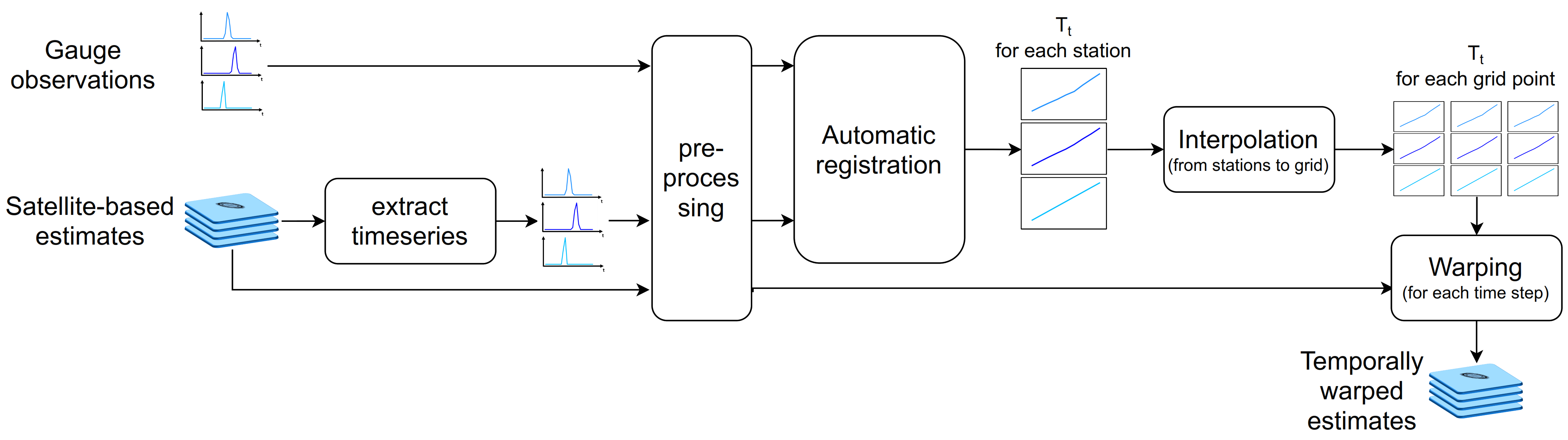
The goal of this article is to investigate the use of warping to correct timing and position error. That is, we apply warping to gauge-adjust a satellite-based estimate with respect to the timing or the position of the rainfall events. For the correction of the position error, we built upon the spatial-warping approach described in [25] and extended it to take into account the temporal dimension of the event. Instead of processing one time step at a time, we considered all the time steps contributing to the event together. This way, they can influence each other. For the time warping, we adapted the spatial warping method to operate with (1D) time series instead of (2D) rainfall fields. Using this method allowed us to compare more fairly the space and time warping. It also leaves open the possibility to combine them at a later stage in order to correct both the position and timing error at the same time. However, that would also be very computationally expensive. Here, as an intermediate step, we considered the time warping separately from the spatial warping. Still, the connection between space and time is not completely ignored in the space and time warping. As mentioned above, in the space warping, the time steps can influence each other. Similarly, we took the spatial dimension into account in the time warping by processing time series of several gauges at once, so that nearby gauges could influence each other.

2. Methodology

In this section, we define the space and time warping and their implementation.

2.1. Spatial Warping

For the spatial warping, we built upon our previous work [25], which used the framework described in [24].

2.1.1. Definitions

Image warping is the distortion of an image by transforming the spatial coordinates. In our case, the image is a gridded rainfall estimate u defined on a domain $D\subset {\mathbb{R}}^2$. It is warped by applying a mapping function $T:(x,y)\in {\mathbb{R}}^2\mapsto \left(T_x(x,y),T_y(x,y)\right)\in {\mathbb{R}}^2$ on the spatial coordinates. That is, for all points $(x,y)\in D$, the warped field is given by:

$$\begin{array}{ccc}\hfill u_{\mathtt{space}}& =& u\left[\left(I+T\right)(x,y)\right]\hfill \\ & =& u\left[x+T_x(x,y),y+T_y(x,y)\right]\hfill \end{array}$$

(1)

where I is the identity function.

The mapping T is found by the image registration. Given two rainfall fields u and v, the goal of the image registration is to find a spatial mapping T such that for all points $(x,y)$ of the domain D:

$$\begin{array}{ccc}\hfill v(x,y)& \approx & u_{\mathtt{space}}\hfill \\ & \approx & u\left[\left(I+T\right)(x,y)\right]\hfill \end{array}$$

(2)

Several mappings can fit this definition, especially in areas without rainfall. Thus, we added additional criteria to characterize a unique optimal mapping:

• $T\approx 0$, i.e., the mapping has to be as small as possible;
• $\nabla T\approx 0$, i.e., the mapping has to be as smooth as possible;
• $\nabla ·T\approx 0$, i.e., the mapping is not shrinking or expanding the domain.

2.1.2. Automatic Registration

For the image registration, we used a similar method as described in [24]. It is an automatic registration method that only needs the two rainfall fields u and v as inputs. It does not require any manual selections of corresponding points.

The method is based on the minimization of the cost function J with respect to the mapping T. For a given time, let u be the first guess and v the target rainfall fields. The cost function J can be divided in two parts: an observation term $J_o$ and a background term $J_b$ (see Equation (3)). The observation term is the error between the warped field $u_{\mathtt{space}}$ and the target field v. The background term corresponds to the three criteria for the optimal mapping. They are translated as weak constraints in this term.

$$\begin{array}{ccc}\hfill J\left(T\right)& =& J_o\left(T\right)+J_b\left(T\right)\hfill \\ \hfill J_o\left(T\right)& =& \parallel v-u\circ (I+T)\parallel \hfill \\ \hfill J_b\left(T\right)& =& C_1\parallel T\parallel +C_2\parallel \nabla T\parallel +C_3\parallel \nabla ·T\parallel \hfill \end{array}$$

(3)

where $C_1$, $C_2$, and $C_3$ are three coefficients determined empirically and $\parallel .\parallel$ is the $L^2-$norm.

The minimization problem is solved iteratively for the mapping T defined on increasingly fine grids. That is, the mapping is first defined on a very coarse grid. The result of the minimization on this coarse grid is used as the first guess for the next iteration with T defined on a finer grid. We iterated for a chosen number of iterations I. The iterative approach has two advantages. First, it is computationally less expensive to solve several minimization problems on coarse grids than one on a high-resolution grid. Second, increasing the resolution of the grid while decreasing the smoothing reduces the local minima problem. The same algorithm was used in [25], where it was described with more details.

Irregularly Spaced Observations

The automatic registration method described above assumes that both fields u and v are defined on the same regular grid. However, that is not always the case in practice. For example, rain-gauge data are irregularly spaced observations, and so they cannot be used directly.

In the case of irregularly spaced observations, we slightly modified the method. First, we interpolated the data onto the same regular grid, using kriging. The krigged field was then used as input for the automatic registration. For this step, we used an ordinary kriging method with a square root transform in combination with an exponential variogram (with a sill of 1.0 mm${}^2$/h${}^2$, a range of $1.5^{\circ }$, and a nugget of 0.01 mm${}^2$/h${}^2$). Second, the cost function j was modified such that areas without observations were not taken into account. This was done by adding a mask function M in the observation term:

$$\begin{array}{ccc}\hfill J\left(T\right)& =& \parallel M·(v-u\circ (I+T))\parallel +C_1\parallel T\parallel +C_2\parallel \nabla T\parallel +C_3\parallel \nabla ·T\parallel \hfill \end{array}$$

(4)

where · is the elementwise matrix multiplication. The mask function was set to 1 within a given perimeter of the observations, and to 0 everywhere else. This way, the observation error $v-u\circ (I+T)$ at grid points far from any observations did not weigh in the cost function.

Time Dimension

In practice, we have rainfall data at several time step. That is, we have two rain fields $u_k$ and $v_k$ for each time k ($k=1,\dots ,K$). In [25], the automatic registration and the warping were applied to a single time step. One could consider the time steps independently and apply that approach to every time step separately. Here, we considered an alternative approach that takes into account the temporal dimension of the rainfall event. We assumed that, during a rainfall events, the mappings of two consecutive time steps are linked. That is, each time step has a different mapping $T_k$, but the mappings cannot vary too much from one time step to the next. This was done by solving the minimization problem for all the mappings $T_k$ at once and adding an additional background term that links the mappings through a correlation matrix. The cost function becomes:

$$\begin{array}{ccc}\hfill J(\left[\begin{array}{c}{T}_1\\ T_2\\ ...\\ T_K\end{array}\right])& =& \parallel \left[\begin{array}{c}{\tilde{v}}_1-{\tilde{u}}_1\circ (I+T_1)\\ {\tilde{v}}_2-{\tilde{u}}_2\circ (I+T_2)\\ ...\\ {\tilde{v}}_K-{\tilde{u}}_K\circ (I+T_K)\end{array}\right]\parallel +C_1\parallel \left[\begin{array}{c}{T}_1\\ T_2\\ ...\\ T_K\end{array}\right]\parallel +C_2\parallel \left[\begin{array}{c}\nabla T_1\\ \nabla T_2\\ ...\\ \nabla T_K\end{array}\right]\parallel +C_3\parallel \left[\begin{array}{c}\nabla ·T_1\\ \nabla ·T_2\\ ...\\ \nabla ·T_K\end{array}\right]\parallel \hfill \\ & & +c_t\parallel \left[\begin{array}{c}{T}_1-T_2\\ T_2-T_3\\ ⋮\\ T_{k-1}-T_k\end{array}\right]\parallel \hfill \end{array}$$

(5)

The coefficient $c_t$ determines how strong the connection is between time steps. The minimization problem is solved for all the mappings $T_k$ at the same time.

2.1.3. Workflow

The workflow of the spatial warping method is summarized in Figure 1. If the rainfall data for the target field are not gridded (e.g., measurements from rain gauges), we start by kriging the point observations into the regular grid. Then, both fields u and v undergo preprocessing. The preprocessing consists of two steps:

• The light precipitation is removed from the fields. Practically, all rainfall below 1 mm/h was set to zero. The automatic registration needs the fields u and v to be similar. Low precipitation has a higher spatial variability and is more difficult to estimate. Thus, low precipitation in the two fields can be very different and so is less suitable for the automatic registration. A minimum threshold of 1 mm/h was chosen as a reasonable value, which in the analysis gave good results;
• A padding area is added around the domain. This area is filled with zero precipitation. It is used to avoid unrealistic distortion in the mapping near the boundary. These distortions are due to precipitation near the border and the constraint ensuring that no grid nodes can leave the domain.

The preprocessed field are used as inputs for the automatic registration, which returns a mapping. This mapping is then applied to the original rainfall field (not the preprocessed one).

The regulation coefficients and the number of steps in the automatic registration were chosen empirically. We set the coefficients to $C_1=0.1$, $C_2=C_3=1$, and $c_t=0.3$ and the number of steps to $I=4$. The same parameters were used in the two case studies. The sensitivity of the results with respect to these parameters is discussed later in Section 5.1.

2.2. Time Warping

2.2.1. Definitions

In the case of temporal warping, the inputs u and v are time series defined on a domain $D=\left[t_{min},t_{max}\right]\subset \mathbb{R}$. The warped time series is obtained by applying a mapping function $T_t$ on the time coordinates:

$$\begin{array}{ccc}\hfill u_{\mathtt{time}}\left(t\right)& =& u\left[(I+T_t)\left(t\right)\right]\hfill \\ & =& u\left[t+T_t\left(t\right)\right]\hfill \end{array}$$

(6)

where I is the identity function.

The mapping $T_t$ is derived by a (1D) registration method. The goal of the registration is to determine the temporal mapping $T_t:t\in \mathbb{R}\mapsto T_t\left(t\right)\in \mathbb{R}$ such that, $\forall t\in D$,

$$\begin{array}{ccc}\hfill v\left(t\right)& \approx & u_{\mathtt{time}}\hfill \\ & \approx & u\left[t+T_t\left(t\right)\right]\hfill \end{array}$$

(7)

There can be several mappings $T_t$ that meet the requirement $v\approx u_{\mathtt{time}}$. Especially in time periods without rainfall, the mapping $T_t$ is not unique. We define two criteria to characterize a unique optimal mapping:

• $T\approx 0$, i.e., the mapping has to be as small as possible;
• $\nabla T\approx 0$, i.e., the mapping has to be as smooth as possible.

These two criteria are similar to the first two criteria used for the spatial registration in Section 2.1.1. For the temporal cases, we did not have a divergent-free constraint as we had in the spatial one.

2.2.2. Automatic Registration

The automatic registration method for the time warping is similar to the one used for the spatial warping (described in Section 2.1.2). The spatial registration method was adapted to the 1D data (i.e., time series) and the new constraints. The time automatic registration only needs the time series u and v as inputs. It does not require any manual selection of matching points or features. A downside of such a method is that the input signals need to be similar enough for it to work.

The registration is based on the minimization of a cost function J with respect to the mapping $T_t$. The cost function is composed of two terms. The first one ($J_o$) represents the error between the warped time series $u_{\mathtt{time}}$ and the target time series v. The second one ($J_b$) is a background term that consists of the two criteria for the optimal mapping.

$$\begin{array}{ccc}\hfill J\left(T\right)& =& J_o\left(T\right)+J_b\left(T\right)\hfill \end{array}$$

(8)

$$\begin{array}{ccc}\hfill J_o\left(T\right)& =& \parallel v-u\circ (I+T)\parallel \hfill \end{array}$$

(9)

$$\begin{array}{ccc}\hfill J_b\left(T\right)& =& C_1\parallel T\parallel +C_2\parallel \nabla T\parallel \hfill \end{array}$$

(10)

where $C_1$ and $C_2$ are two coefficients determined empirically and $\parallel .\parallel$ is the $L^2-$norm.

As for the spatial 2D case, the minimization problem is solved iteratively, for $T_t$ defined on increasingly fine grids. The algorithm of the time registration is similar to the one of the spatial one.

Spatial Dimension

In practice, we will obtain rainfall observations from several stations. Thus, we will have two time series $u_j$ and $v_j$ for each station j ($j=1,\dots ,J$). The easier approach is to consider that all the stations are independent and process each pair of time series separately. Here, we took a different approach and assumed that the mappings of the different stations are linked though space. That is, every station has a different mapping, but the mappings of neighboring stations are similar. The automatic registration method described above was modified accordingly. All the mappings $T_j$ are found at once by solving one minimization problem. They are linked through a correlation matrix based on distance (derived from a variogram). This is done by adding an extra background term. The cost function is modified as follows:

$$\begin{array}{ccc}\hfill J(\left[\begin{array}{c}{T}_1\\ T_2\\ ...\\ T_K\end{array}\right])& =& \parallel \left[\begin{array}{c}{\tilde{v}}_1-{\tilde{u}}_1\circ (I+T_1)\\ {\tilde{v}}_2-{\tilde{u}}_2\circ (I+T_2)\\ ...\\ {\tilde{v}}_K-{\tilde{u}}_K\circ (I+T_K)\end{array}\right]\parallel +C_1\parallel \left[\begin{array}{c}{T}_1\\ T_2\\ ...\\ T_K\end{array}\right]\parallel +C_2\parallel \left[\begin{array}{c}\nabla T_1\\ \nabla T_2\\ ...\\ \nabla T_K\end{array}\right]\parallel \hfill \\ & & +c_s\sum _{j_1,j_2\in J|j_1\ne j_2}c(d_{j_1,j_2})\parallel T_{j_1}-T_{j_2}\parallel \hfill \end{array}$$

(11)

where $d_{j_1,j_2}$ is the distance between the stations $j_1$ and $j_2$. The influence function c determines the strength of the connection between the stations based on their distance. This strength is given on a scale of 0 to 1. The function is based on an exponential variogram with a range of 150 km and no nugget. The spatial regulation coefficient $c_s$ defines the weight of the spatial background term in the cost function.

2.2.3. Workflow

In practice, we want to adjust satellite-based estimates using gauge measurements. The satellite estimates are given on a 2D grid and do not correspond to gauge locations. Thus, the first step is to extract the time series at the gauge locations from the series of rainfall fields given on this grid. Once we have the two time series for each station (one v from the gauge and one u from the satellite estimates), they go through a preprocessing step, which consists of resampling. The time series have a low resolution of 1 h, and they were resampled at a higher resolution of 6 min using linear interpolation. This has two advantages. First, by increasing the number of grid points, we prevent extreme shrinking of the time interval (i.e., of the grid cells). Second, it prevents the warping to decrease the peak intensity artificially by sampling away from it. The resampled time series were used as the input for the automatic registration.

The automatic registration can be tuned by several parameters: the regulation coefficients and the number of step. They were chosen empirically. The regulation coefficients were set to $C_1=0.1$, $C_2=1$ and $c_s=1$. These coefficients are similar to the ones used in the spatial registration (see Section 2.1.3). The number of steps was set to $I=3$. These parameters and their impact on the results are discussed in Section 5.1.

The automatic registration provides the temporal mappings at the station locations. Our goal was to warp the full satellite estimates. That is, we wanted the temporal mapping for each node of the 2D grid. They were obtained by kriging the mappings. We used the same exponential variogram as the one used for the spatial background term of the cost function (i.e., with a range of 150 km and no nugget). Then, the mappings were used to warped the (resampled) time series of each node.

The complete workflow of the method, from the time series extraction to warping itself, is summarized in Figure 2.

3. Case Studies

The warping methods were applied to two case studies. A synthetic case was used to evaluate the accuracy of the methods when the “true” rainfall was known. The second case was a rainfall event occurring in southern Ghana during the monsoon season. This case allowed us to investigate the potential of the methods when applied to real noisy data.

3.1. Synthetic Case

The synthetic case was used to investigate the accuracy of the automatic registration for the time and space warpings. The synthetic case was generated by 3D ellipses on a regular grid. The two input fields (the first guess and the target) both had one rainfall event moving toward the southwest, as can be seen in Figure 3. They had the same maximum of 50 mm/h for the rainfall peak, but different positions, timings, and paths. This was done by giving the ellipses different positions and orientations. The peak of the rainfall events differed by ∼50 km and by 2 h. They also differed by the propagation direction and speed. The event was moving at ∼40 km/h in the first guess and at ∼47 km/h in the target field.

In a real case, the first guess would be a satellite-based estimate, and the target field would be observations from radar or gauges, for example. When using gauge measurements, the “true” rainfall is only known at the station’s locations. We simulated this case by extracting time series from the “true” rainfall field. The locations of the fictive stations followed the configuration of the gauge network used in the southern Ghana case (described in Section 3.2) and are represented by circles in Figure 3. These time series were used as the input v in the automatic registration. We used linear interpolation to derive the rainfall values at the gauge locations. The same method was used to extract the time series u from the first guess before the preprocessing step (see Figure 2). We denote by $u_{grid}$ and $v_{grid}$ the two input fields from which the time series u and v were extracted.

3.2. Southern Ghana Case

The southern Ghana case was used to test the automatic registration and the time warping on real precipitation data. In this study case, the first guess was the satellite-based estimate IMERG-Late [26] and the target was gauge data from the TAHMO network [27,28,29]. We assumed that the gauge measurements were more accurate, but that the spatial variability of the rainfall was better represented by the IMERG estimate because of its higher resolution and the relative low density of the gauge network in the area. Our goal was to use the gauge data to correct the IMERG estimate with respect to time while preserving its higher spatial variability.

The study area is located in southern Ghana and covers the Ghanaian cocoa region. This area was selected because of the important number of TAHMO stations located in it. The domain corresponds to a square of $3.7^{\circ }$ latitude by $3.7^{\circ }$ longitude, that is to $37\times 37$ grid points for the IMERG estimate. We selected a 25 h time period during the main rainy season of 2018 with a resolution of 1 h (of accumulated rainfall). The period extends from 06:00 22 April to 06:00 23 April 2018 (included) and contains one rainfall event. We used the data from 65 TAHMO stations that are located in the domain and have a complete record for this time window (Figure 4). This is roughly equivalent to one station per 2595 km² on average.

Figure 5 shows the one-hour accumulated rainfall according to the IMERG-Late estimates and the TAHMO measurements for the selected domain and time window. In both datasets, we can observe one main rainfall event, but with different characteristics. The rainfall peak is higher in TAHMO measurements (53.45 mm/h) than in IMERG-Late (19 mm/h). The position and the timing of the peak differ as well. The peak occurs at 18:00 according to TAHMO, while it has a larger time span in the IMERG estimates (18:00 and 19:00). In the latter, the peak is located more northeast than in TAHMO. There is a spatial shift of about 55 km in the peak’s position at 18:00.

4. Results

In this section, we show the impact of the space and time warping methods on the two case studies.

4.1. Synthetic Case

4.1.1. Mappings’ Comparison

Spatial Mappings

The automatic registration provides a mapping $T_s$ for each time steps. The mappings are shown in Figure 6 for twelve of the time steps. We only show the mappings at some selected time steps for the sake of clarity. At the other time steps, the mappings were much smaller or zero, due to the absence of precipitation in the target field v.

It can be noticed from Figure 6 that the largest distortions occurred in the center of the domain where the rain event was located. The relatively smaller distortion near the boundary was due to the padding area and the first regulation term of the cost function, which ensured that the mapping was as “small” as possible. The second term ensured that the mapping was as “smooth” as possible, avoiding abrupt distortion in the mappings. It was responsible for the smooth transformation between the larger distortions in the center and the areas with no or few distortions. The goal of the third term was to avoid the grid cell shrinking or expanding. The temporal regulation term ensured a smooth transition between the time steps. One clear effect of this term was a nonzero mapping at Time Step 9. If the time steps would have been treated separately, this mapping would have been zero since there was no precipitation in the target field v at this time. Thus, it prevented unnatural temporal distortion.

Time Mappings

The automatic time registration provides a mapping $T_t$ for each of the stations. Figure 7 shows the mappings for three of these stations, as well as the corresponding warped fields. The positions of all the stations mentioned in this article, including these three, are indicated in Figure A1. The mappings for the whole domain were obtained by kriging and are displayed in Figure 8.

At all stations, the mapping was null at the last time step (Figure 7). This was due to the constraint that no node could leave the domain. The mappings $T_t$ cannot be strictly negative at this time step without violating this constraint. Similarly, the mappings cannot be strictly positive at Time Step 0 (see the southern Ghana case in Section 4.2). The distortion was smaller at the beginning of the time series, before the rainfall occurred. This was due to the first regulation term that ensured that the mappings were as small as possible. The second regulation term ensured that the mappings were as smooth as possible.

The time mappings $T_t$ provided by the automatic registration were krigged onto the 2D grid. Figure 8 allows us to examine their spatial variation. The chosen approach for the automatic registration authorized variation in space (each station has its own mapping), while keeping some spatial consistency due to the spatial regulation term. This extra regulation term prevents two stations next to each other from having too different mappings. Large differences between neighboring stations would impact the shape of the event in the warped field and could lead to unnatural distortion. The spatial regulation term in the automatic registration limited that effect while still allowing some spatial variation.

4.1.2. Validation

The spatial- and time-warping methods act respectively on the spatial coordinates and the time coordinates. They do not act directly on the intensity. However, by modifying the position or the timing of the rainfall event, they also impact the intensity error. We used the Root-Mean-Squared Error (RMSE), Mean Absolute Error (MAE), and Pearson correlation coefficient to evaluate the intensity error.

Table 1. Statistics before and after warping compared to the “truth” v. The statistics are computed over the whole domain and all time steps.

	Before	After
		Spatial Warping	Time Warping
RMSE (mm/h)	5.62	2.65	2.76
MAE (mm/h)	1.65	0.64	0.73
Correlation	0.12	0.79	0.76

gives quantitative measures of the error before and after the warping. One can see that both warping methods significantly improved the statistics. The RMSE and the MAE were divided by at least two, while the correlation increased from 0.12 to 0.79 and 0.76 for the spatial and time warpings, respectively. The differences between the two warpings was relatively small, with the spatial warping having slightly better statistics.

The synthetic case was built with both a timing and a position error between the fields u and v. Part of the position error can be interpreted as timing error and vice versa. Thus, we examined the impact of both warping methods on the position and timing error.

We define the position error as the distance between the rainfall peaks in the first guess and the truth, the peak being the pixel with the maximum rainfall at a given time. The position error before and after warping is visualized in Figure 9. Figure 9a shows the trajectory of the rainfall peak according to the “truth” (v), the original fields u, and the warped fields. One can clearly see an improvement of the trajectory after the spatial warping. It is more difficult to observe the impact of the time warping. The trajectory after the time warping seems very similar to the original one. However, by moving the peak forward in time, it reduced the position error as well. This can be seen in Figure 9b, which shows the position error at each time step (with nonzero rainfall). After the time warping, the position error decreased by about 20 km at most time steps. As expected, the decrease of the position error was more important with the spatial warping. The position of the rainfall peak matched perfectly the one from the “truth” at Time Steps 14 to 17. These time steps were the ones with the highest rainfall peaks. The higher position error at the other time steps could be partially due to the interpolation of the stations. The rainfall peak might not be located exactly at the same location in the “truth” and in the krigged field used as input for the automatic registration.

The spatial correction is evaluated more quantitatively in

Table 2. Average position error (in km) before and after warping. The average is over all time steps at which the rainfall peak (in the target field v) is above a certain threshold.

Threshold (peak)	Sample Number	Before	After
			Spatial Warping	Time Warping
>1 mm/h	n = 10	98.54	15.78	73.11
>10 mm/h	n = 7	90.76	7.37	63.54
>20 mm/h	n = 5	89.54	8.10	60.80

. We computed the average position error over several time steps with the peak above a certain threshold. The spatial warping considerably reduced the position error. The position error went from 98.54 km on average to 15.78 km for the 1 mm/h threshold. The error decreased when the threshold increased, suggesting that the spatial warping is more efficient at time steps with higher rainfall rate. The error was divided by eight over all times with some rainfall, but by more than ten when only considering times with more than 10 mm/h of precipitation. The time warping method also had a positive if not more limited impact on the position error. It decreased by about 30 km for all thresholds.

The timing error is defined as the time difference between the peaks in the fields u and v, the peak being defined as the time step with the maximum rainfall. Figure 10 shows the timing error over the domain before and after warping. Before the warping, the first guess u was early with respect to the truth v. The timing error increased from 0 h in the west to 4 h in the east. Both warping methods improved the timing of the rainfall event in u. The spatial warping led to the largest improvement. The time warping had a more limited improvement than expected. This could be partially due to the resampling. The automatic registration uses time series resampled at a 10 min resolution. For a fair comparison with the spatial warping, the warped field $u_{\mathrm{time}}$ was resampled back to the original 1 h resolution. For the spatial warping, one can notice a small area near the eastern boundary that has a much higher timing error than the rest of the domain. This area does not have gauges and, so, is not well represented by the krigged field used as input for the automatic registration.

Table 3. Average absolute timing error before and after warping. The average is over all pixels recording at least one time step with more rainfall than a certain threshold according to v (and with nonzero rainfall according to u).

Threshold (peak)	Sample Number	Before	After
			Spatial Warping	Time Warping
>1 mm/h	n = 1128	2.21	0.50	0.77
>10 mm/h	n = 565	2.07	0.22	0.67
>20 mm/h	n = 315	2.07	0.17	0.59

provides the average absolute timing errors before and after spatial warping for different rainfall thresholds. As observed in Figure 10, both warping methods decreased significantly the timing error with the spatial warping, leading to the largest improvement. The spatial warping divides the timing error by a factor four for the threshold of 1 mm/h and by more than ten for the 20 mm/h threshold. The timing error was divided by about three for all thresholds by the time warping.

4.2. Southern Ghana Case

For the southern Ghana case, we did not know the “truth” as we did for the synthetic case. Thus, we used a Leave-One-Out-Validation (LOOV) to evaluate the accuracy of the method [30]. That is, we removed one of the 65 TAHMO stations from the input data to use for validation. We repeated this operation 65 times, once for each station.

For comparison, we ran a second experiment using all the stations in the input v. We call this second experiment “All”. The results of the “All” experiment were not independent of the validation data. However, it provided insight into the impact of the gauge network configuration on the efficiency of the method and on what is the “best” possible results with the current network.

4.2.1. Mappings’ Comparison

Sensitivity of the Spatial Mappings

From the LOOV experiment, we obtained 65 mappings $T_s$ based on 65 different interpolated fields used as input. With this set of 65 different inputs v, the LOOV experiment gave us insight into the sensitivity of the automatic registration to the input data.

We looked at the average mapping (over the 65 realizations) and the corresponding standard deviation. The average mappings are shown in Figure 11 for some selected time step. The largest distortions occurred in the rainy areas (see Figure 5). The distortions became smaller further away from the rainy peaks, due to the first regulation term of the cost function, which ensured a mapping as “small” as possible. The second regulation term ensured that the mapping was as “smooth” as possible and was responsible for the smooth transition between these areas. The third regulation term penalized grid cell shrinkage or expansion. The temporal regulation term was responsible for the smooth transition of the mapping from one time to the next. Without this term, the mapping would be null at 15:00 and 17:00, since the gauges did not record any precipitation at these times.

The standard deviation of the “LOOV” experiment is shown in Figure 12. On the left, one can see the average standard deviation (over space), as well as the maximum, for each time step. The standard deviation was zero at time steps far away from the rainy times. This was due to the fact that the mappings were all zero at these time steps (because to the first regulation term). The standard deviation was larger in the longitudinal direction than in the latitudinal one. The average standard deviation going up to 0.018${}^{\circ }$ in the latitudinal direction and up to 0.025${}^{\circ }$ in the longitudinal direction. The maximum standard deviation went up to 0.10${}^{\circ }$ in the latitudinal direction and up to 0.14${}^{\circ }$ in the longitudinal direction. This can also be seen when looking at the maximum (in time) standard deviation at each grid cell (Figure 12a). At most grid cells, the maximum standard deviation was larger in the longitudinal direction than in the latitudinal one.

Sensitivity of the Time Mappings

We examined the impact of the individual station on the mappings $T_t$ by comparing the “All” and the “LOOV” experiments at the station locations in Figure 13 (see Figure A1 for the position of these stations within the domain). For all stations, the distortions were larger in the center of the time series and became smaller at the beginning and at the end, away from the rainfall event. This was due to the first regulation term ensuring that the mapping was as “small” as possible and to the boundary condition requiring that no node leaves the domain (thus, the mapping cannot be strictly positive at Time 0). The second regulation term ensured a smooth transition between the time steps. At some stations, the two experiment “All” and “LOOV” gave similar mapping (e.g., for TA00277, TA00012, or TA00181). However, at other stations, there were noticeable differences. For example, at station TA00312, the maximum distortion was around Time 8 for the “All” experiment, while it was around Time 19 in the “LOOV” experiment.

In practice, in order to warp the entire domain, and not just the stations, we krigged the mappings from the stations to the 2D grid on which IMERG is defined. Theses mappings were then applied to the time series of the grid points. For the “LOOV” experiment, we repeated the kriging for the 65 realizations and obtained 65 sets of mappings. The average mappings (over the 65 realizations) are shown in Figure 14. The mappings obtained with the “All” experiment were very similar to these average mappings, and so are not shown here. The areas and times with the most important deviations did not necessarily correspond to the ones with the highest rainfall amount. The distortions became smaller away from the stations due to the kriging. Far away from the stations, the krigged mapping tended to the mean.

The standard deviation of the “LOOV” experiment (Figure 15) gave us insight into the sensitivity of the mappings with respect to the gauge network. The standard deviation varied in both space and time. The higher standard deviations were localized around specific stations and decreased away from them. The areas and times with the highest standard deviation generally corresponded to the ones with the largest mappings (Figure 14). The highest standard deviation (0.5 h) was reached at time 00:00. The standard deviation was thus smaller than the original temporal resolution of the data (1 h), but larger than the resolution of the resampled time series (0.1 h).

4.2.2. Validation

In contrast to the synthetic case, we did not know the “truth”. It was thus more difficult to evaluate quantitatively the impact of the warping methods on the rainfall estimate. We used the gauge observations from the TAHMO network as the validation dataset. The results of the “All” experiment were not independent of the validation data, since the TAHMO stations were used both as input to the automatic registration (after kriging) and for the validation. However, this experiment provided insight into the “best” possible results. We used the “LOOV” experiment to have a more independent validation.

Table 4. Statistics before and after warping compared to the station measurements. The results are shown for the two experiments (“LOOV” and “All”) and the two warping methods. The statistics are computed over all stations and all time steps.

	Before	Spatial Warping		Time Warping
		All	LOOV	All	LOOV
RMSE (mm/h)	1.89	1.39	1.49	1.51	1.51
MAE (mm/h)	0.20	0.13	0.14	0.12	0.13
Correlation	0.18	0.70	0.62	0.66	0.66

provides the statistics before and after warping for the two experiments. One can notice that both warping methods improved the RMSE, the MAE, and the correlation coefficient. For the “LOOV” experiment, the RMSE decreased by about 0.4 mm/h and the MAE by about 0.06 mm/h. The most significant improvement is shown by the correlation that went from 0.18 to 0.62 after the spatial warping and to 0.66 after time warping. For both warping methods, the “All” experiment had slightly better statistics than the “LOOV” ones. This was to be expected since the validation data were not independent of the input data. However, the difference between the two experiments remained small.

Position Error

As mentioned above, we did not know the “truth” on the whole grid, only at the station locations. It was thus more difficult to compute the position error. For the spatial warping, the gauge measurements were krigged onto the grid before the automatic registration. We used this krigged field as reference for the position error. Thus, the position error had to be considered with caution, since the kriging added uncertainty. From the “LOOV” experiment, we obtained 65 sets of mappings, one for each realization, which made the computation of the peak position ambiguous. Moreover, the average mapping from the “LOOV” experiment was very similar to the one from the “All” experiment. Thus, we only computed the position error for the “All” experiment.

Figure 16 shows the position errors before and after warping at each time step (with more than 1 mm/h of rainfall). The spatial warping significantly improved the position error at all time steps. The lowest position error was achieve at 18:00, the time step with the highest recorded rainfall according to the gauges. The time warping had a more mixed impact on the position error. At 20:00, the position error was significantly reduced; however, it increased at several other time steps. The largest deterioration was observed at 22:00. This deterioration was due to a second event in the southern part of the domain that was detected by IMERG, but not by TAHMO. In the warped fields, this second event was identified as the peak, while the krigged field still identified the central event as the peak.

Table 5. Average position error (km) before and after warping for the “All” experiment. The average is over all time steps at which the peak (in v) is above a certain threshold.

Threshold (peak)	Sample Number	Before	Spatial Warping	Time Warping
>1 mm/h	n = 9	124.53	76.90	114.90
>5 mm/h	n = 4	82.45	21.23	65.62
>10 mm/h	n = 2	68.32	22.20	74.58

gives the position error averaged over the time steps for different rainfall thresholds. The spatial warping had a clear positive impact on the position error. The decrease of the error was more important for the 5 mm/h and 10 mm/h threshold than for the lowest one (1 mm/h). The time steps with the higher rainfall seemed to benefit more from the spatial warping. As observed in Figure 16, the time warping had a small and mixed impact on the position error. It decreased the average error for the two lowest thresholds, but increased for the 10 mm/h one.

Timing Error

The timing error of the rainfall peak between the stations and the satellite estimates is shown in Figure 17 (only for the stations with a peak above 0.1 mm/h). At most station locations, the rainfall peak in IMERG was late compared to the gauges. After warping, the absolute timing error decreased by one or two hours at most stations for both experiment and both methods (see Figure 18). Among the 15 stations with more the 0.1 mm/h (in both IMERG and TAHMO time series), only two showed deterioration after warping. The timing error at station TA00047 (at $6.3^{\circ }$ N, $1.4^{\circ }$ W; see Figure A1) deteriorated by one hour after time warping and by two hours after spatial warping. This could be explained by the low intensity of the rainfall peak (0.1 mm/h and 0.4 mm/h according to TAHMO and IMERG, respectively) and by the shape of the time series (with two peaks). In the “LOOV” experiment with the time warping, a second station showed an increase of the absolute timing error. At this station (TA00276 at $6.5^{\circ }$ N, $2.3^{\circ }$ W, see Figure A1), the shapes of the TAHMO and IMERG time series were slightly different. The peak was near the beginning of the event in IMERG, while it was toward the end in TAHMO. Thus, after time warping, the spans of the event in TAHMO and IMERG matched better, but the peaks were less aligned.

We look at the timing error more quantitatively in

Table 6. Average absolute timing error before and after spatial warping. The average is over all stations recording at least one time step with more rainfall than a certain threshold.

Threshold (peak)	Sample Number	Before	Spatial Warping		Time Warping
			All	LOOV	All	LOOV
>1 mm/h	n = 10	1.10	0.40	0.40	0.10	0.20
>5 mm/h	n = 7	1.00	0.29	0.14	0.00	0.14
>10 mm/h	n = 5	1.20	0.20	0.20	0.00	0.00

, which gives the absolute timing error averaged over the stations recording more rainfall than a certain threshold. Both warping methods improved the timing error. The largest improvement was obtained with the time warping, which even led to a perfect timing for the time steps with higher rainfall peak (for the threshold of 10 mm/h). The results from the two experiments were relatively similar in terms of timing. The “All” experiment gave slightly better results for the time warping. For the spatial warping, both experiment gave the same average timing errors for the 1 mm/h and 10 mm/h thresholds, but the “LOOV” had a lower error for the 5 mm/h one. In general, the average timing error decreased when the threshold increased. For example, the spatial warping divided the error by 2.75 for the lowest threshold and by six for the highest one. The warping methods seemed to favor the higher rainfall rate.

5. Discussion

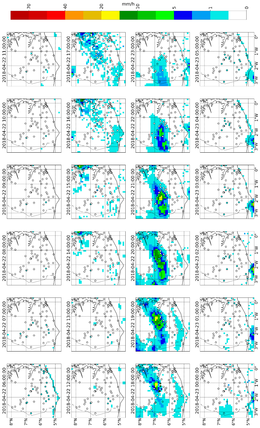
The spatial and time warping methods were evaluated in terms of the position and timing of the rainfall peak and of the intensity of the event for two case studies. The spatial warping method targets the position error, and successfully improved it. The position error was significantly decreased after spatial warping in both cases (see Table 2 and Table 5). The timing error also decreased after the spatial warping (see Table 3 and Table 6). It is hard to distinguish between a time delay or a spatial shift. Part of the timing error can be due to a position error and vice versa. Therefore, by correcting the position, the spatial warping also reduced the timing error. The time warping explicitly corrects the timing error. It was shown that the timing of the event was significantly improved by the time warping for both cases (see Table 3 and Table 6). However, the time warping had a mixed impact on the position error, especially in the southern Ghana case. In the synthetic case, the time warping had a limited, but positive impact on the position. The position error was decreased by about 20 km (which is equivalent to about two grid cells). In the second case study, time warping decreased the position error at certain time steps, but increased it at others. However, the position error has to be interpreted with caution for this case study. There were several time steps with low and scattered precipitation for which the rainfall peak was not well defined because of the several local maxima.

By modifying the position or the timing of the rainfall event, the warping methods also impacted the continuous statistics that reflect the intensity error. The MAE, the RMSE, and the correlation were significantly improved after warping in both cases (see Table 1 and Table 4). The warping methods did not modify the intensity of the event, but they removed the double-penalty part of the error by making the events in the two estimates (here, IMERG-Late and TAHMO) fit better in terms of position and timing. This can be seen by the increase of the correlation after warping.

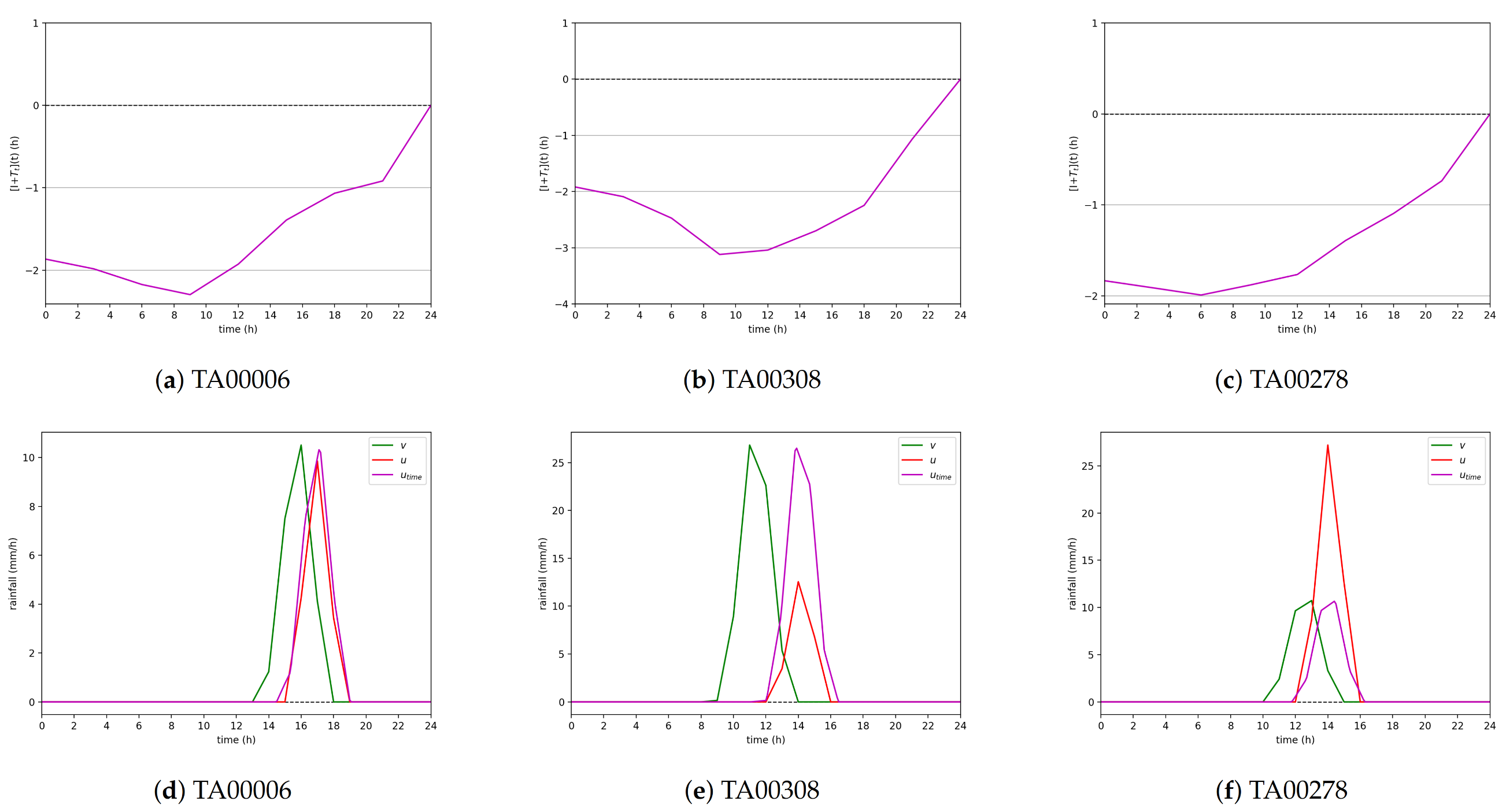
The warping methods seemed to benefit the large rainfall values. This was not due directly to the warping methods, but to the registration methods. The automatic registration is based on the minimization of a cost function. The larger rainfall values had more weight than the low ones in the cost function, and so were corrected with priority during the minimization. The correction of the high rainfall values can be at the detriment of the lower ones. A similar observation can be made for the timing error after time warping. This characteristic can be a drawback for applications for which lower rainfall amounts are important. It also shows a limitation of our validation method, since the timing and position errors are defined with respect to the peak (i.e., the maximum rainfall). They do not take into account the spatial or temporal variation of the lower rainfall. Thus, they can be biased and have to be considered with caution.

The spatial and time automatic registration methods have the advantage of not needing any manual selection. However, this also means that the inputs have to be similar enough for them to perform correctly. This condition is the main limitation of the warping methods. We do not have clear criteria to determine beforehand if the inputs are similar enough. However, there are some minimum conditions, such as having the same number of events. So far, we have used a visual inspection of the input data to assess their similarity. A next step will be to apply this method to other cases, involving different rainfall regimes. More study cases, including extreme ones, are needed to determine the boundaries within which the automatic registration succeeds and to determine “feasibility” thresholds.

The spatial warping method used in this paper built upon previous work in [25]. The main difference was the processing of several time steps at the same time in the automatic registration. In [25], the automatic registration was applied to one time step. To warp the entire rainfall event, one would need to apply the registration to each time step separately. Processing several time steps at the same time allowed us to add an assumption on the relationships of the mappings through time. This was done by adding an additional regulation term in the cost function. This term links the mappings through time, ensuring the time consistency of the mappings.

The spatial automatic registration used in [25] and in this article was based on the one described in [23,24]. Reference [24] described a data assimilation method based on morphing in order to assimilate radar precipitation data into a numerical weather model. However, they did not implement it or apply it to actual rainfall data. We modified and extended their automatic registration function. The first difference is the type of observation data. We used nongridded gauge measurements as observations instead of gridded radar data. Using nongridded data introduces additional uncertainties since we have to interpolate. The cost function was modified accordingly, so that it was not too influenced by areas without gauges. The second difference is the optimization method: they solved the minimization problem iteratively for one grid point at the time, while we solved it for all grid points together. The third main difference is the extension to take into account several time steps at a time.

As mentioned in the Introduction, time or spatial warping methods have been applied on rainfall data in previous works, but not for position and timing correction. For example, dynamic time warping has been used to classify rainfall time series or to measure dissimilarities between them [8,9,10,11,12]. Spatial warping or similar methods have been used for position correction in the framework of data assimilation into numerical weather models. However, they have not been applied on rainfall, but other weather-related variables [15,16,17,18,19,20]. An exception is [21], in which they used a feature calibration and alignment method, similar to spatial warping, to adjust a satellite-based rainfall estimate with respect to radar observations. There are three main differences between their method and the spatial warping described in this article. First, they corrected both the intensity and the position, while we only corrected the position. Second, they processed each time step individually, while we processed all the time steps in the time window at once. This allowed us to take into account the temporal relationship between the displacement fields of the different time steps. Third, they used radar data that were gridded, while we used nongridded gauge observations.

5.1. Parameters Influencing the Warping

The mappings were derived from the automatic registration, which can be tuned by several parameters. These parameters thus impacted the mappings and then the warped fields. The background term of the cost function consists of several regulation terms corresponding to properties characterizing the “optimal” mapping. These terms are weighted by the regulation coefficients $C_1$, $C_2$, $C_3$, $c_t$, or $c_s$. The impact of the coefficients on the mappings and warped fields was examined for the synthetic case (not shown here; see [31]). The regulation terms mainly affect the area or times with no or low rainfall, and so have a limited impact on the warped fields in terms of continuous statistics and of the position and timing errors. Very large regulation coefficients are needed for them to have an effect on larger rainfall values (i.e., more than 5 mm/h). Nevertheless, they had a visible and valuable effect on the mappings. For example, the “smoothness” property controlled by the coefficient $C_2$ prevents nonphysical discontinuity in space (time) for the spatial (time) method. For the spatial warping, the low precipitation is removed in the preprocessing step; thus, this property ensures that it is moved along with the higher rainfall values.

Another parameter influencing the automatic registration is the number of steps I. This number controls two things: the smoothing of the input data and the resolution of the mappings. Thus, a higher number of steps I means that more details are taken into account and that mappings themselves have more details. On the other hand, increasing I also increases the computational cost, since the number of variables in the minimization problem increases exponentially with I. For example, for the spatial registration, the first step (i.e., $i=1$) took 20 s, the second one more than 2 min, the third one 17 min, and the fourth one 47 min. Similarly, for the time registration, the first step ran in less than 6 s, while the third one needed almost a minute. In our case studies, with 65 stations, the computational aspect was not a problem for the time registration, but it could become more critical for cases with more stations.

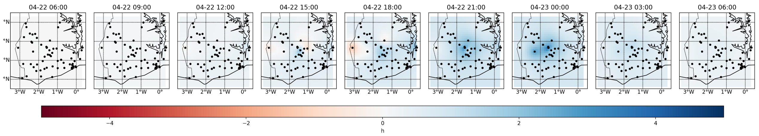
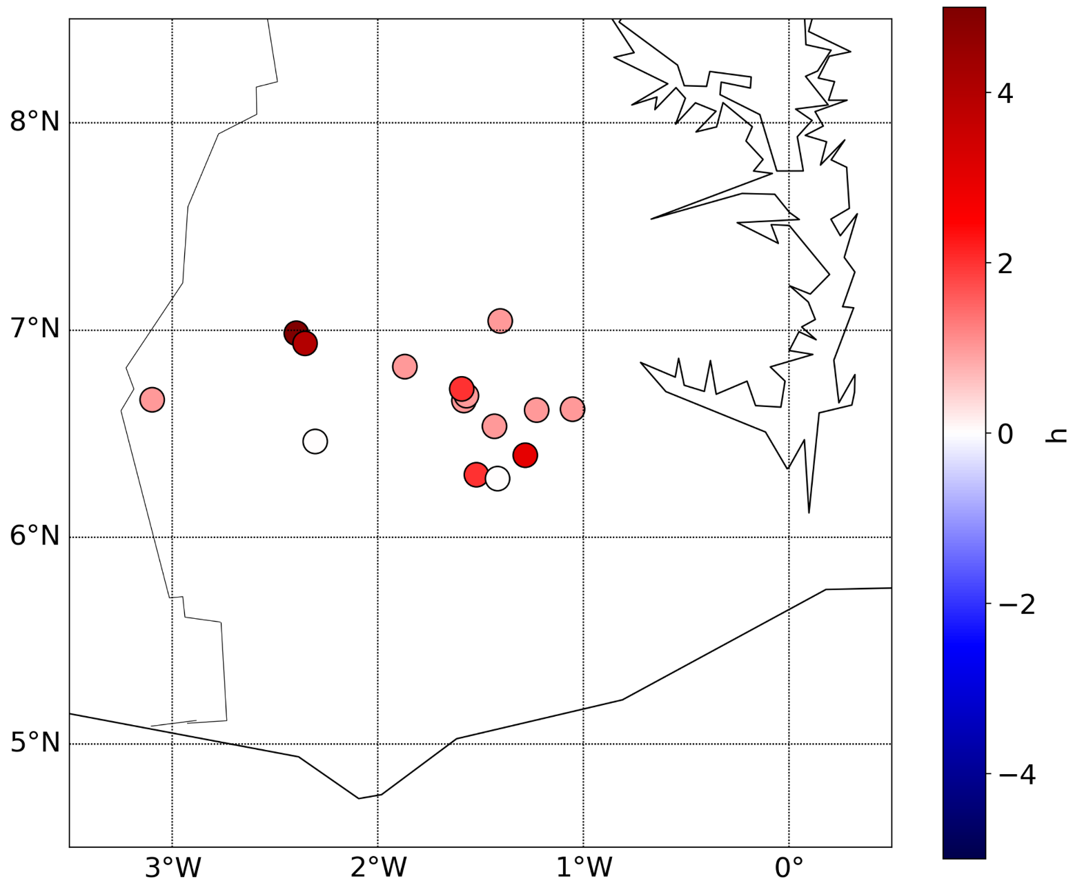
When using nongridded data, there is another important step that influences the results: the interpolation. In the case of the spatial warping, the measurements from the stations have to be interpolated onto a regular grid before being used in the automatic registration. This step introduces some interpolation errors, especially in the areas far from the stations. Depending on its position, the rainfall event was more or less well captured by the stations and so represented by the interpolated field. This can be seen by comparing the “LOOV” and “All” experiments in the southern Ghana case. The standard deviation of the mappings (across the LOOV) was very low; however, some members did show a large deviation from the mean. That is, some stations had a bigger impact than others on the accuracy of the interpolation and, thereby, on the automatic registration. In the two cases studied here, the rainfall event was relatively well captured by the gauges. In practice, that would not always be the case, depending on the position of the event and on the network configuration. In the case of the time warping, the interpolation occurred after the registration. The mappings at the station locations had to be interpolated on the regular grid of the satellite-based estimates. This step was necessary to be able to warp the entire domain. We chose to use an ordinary kriging method, because it can be used for interpolation and extrapolation and can be linked to the spatial regulation term. The same variogram was used to define the influence function in this regulation term and for the ordinary kriging. However, other interpolation methods could have been used. The study of the impact of other interpolation methods is left for future work.

5.2. Computational Cost and Alternative Methods

Once we have the mappings, applying them to the first guess is straight-forward. The computational cost of the warping methods comes from the automatic registration, and more specifically from the minimization. The cost of the minimization increases with the number of variables. For the spatial registration, the number of variables to be determined depends on the number of steps I and the number of time steps. The number I controls the resolution of the mapping, that is the number of grid points. Thus, the choice of the number of steps is a trade-off between the resolution and the computational cost. The number of variables also increases with the number of time steps to be processed at the same time. Therefore, a way to reduce the computational cost would be to reduce the time window. If it is not possible due to the length of the rainfall event, an alternative would be to use a moving time window. We would then run several smaller minimization problems instead of one large one. Another possibility would be to modify the assumption on the time dimension of the mappings. In the present method, the time steps are processed together so that they can be linked though time. An alternative approach is to assume that the mappings at the different times are independent (as was done in [25]). Then, we have several smaller minimization problems that can be run in parallel. A downside of this approach is that the mapping of two consecutive time steps can be very different. This can cause some nonphysical discontinuities in time, such as a sudden jump of the rainfall position. Another alternative approach is to still process all the time steps together, but to assume they have the same position error and so the same mappings. Then, the number of variables does not depend on the number of time steps. We solved the minimization problem for only one mapping. This would be the least expensive approach since the number of variables does not depend on the number of time steps any more. However, it also has a more rigid assumption. The further the data are from this assumption, the less efficient this approach will be.

Similarly, for the time registration, the number of variables, and so the computational cost, depends on the number of steps I and on the number of stations processed at once. In our two case studies, with 65 stations, the computational cost was not a problem, but could become one for larger cases with more stations. As for the spatial registration, we could then consider alternative approaches. The first one would be to assume that the timing errors of the stations are independent and apply the registration to each station separately. Solving several small minimization problem is faster than solving one large one. Moreover, they could be run in parallel since the stations are independent. However, this approach could lead to nonphysical spatial distortion if the mappings of neighboring stations are very different. The second approach is to assume that all stations have the same position error and so need the same mapping. This approach would be less computationally expensive, but also more rigid. It could also lead to a more limited improvement because of the rigidity of the assumption.

6. Conclusions

The use of warping to correct position and timing errors in rainfall estimates was tested on two case studies. The first one was a synthetic case where the rainfall events were represented by ellipses. It was used to evaluate the warping in a case for which the “truth” was known. The second case was a convective rainfall event over southern Ghana and allowed us to test the warping methods on real datasets.

Both the spatial and the time warping had a positive impact on the rainfall estimates:

• The continuous statistics were significantly improved after the warping either in time or in space, e.g., the correlation went from 0.2 to about 0.6 after either warping for the southern Ghana case;
• The timing error was considerably decreased by both types of warping, sometimes more by the spatial one than by the time one. In the southern Ghana case, the spatial and time warpings decreased the average timing error from 1.1 h to 0.40 h and 0.20 h, respectively. In the synthetic case, the error was reduced from 2.21 h to 0.50 h by the spatial warping, but to 0.77 h by the time warping;
• The position error was decreased significantly by the spatial warping; however, the time warping only had a limited impact on it. The average position error was reduced by about 45 km after spatial warping in the southern Ghana case.

Hence, if both spatial and time warping are able to improve the rainfall estimates (in terms of continuous statistics), the spatial warping is more interesting because of its positive impact on both the position and timing errors. However, the spatial warping is also more computationally expensive.

The main drawback of the warping method comes from the automatic registration method. The first guess and the target (or truth) have to be similar enough for the automatic registration to produce meaningful mappings. In the two cases we studied here, the rainfall events were clearly defined and had a unique peak, which made them very suitable for the automatic registration. However, the registration can fail if the rainfall event from the satellite-based estimate and the one from the measurements are too dissimilar. For example, this happens if they have a different number of peaks. Moreover, the events have to be well captured by the gauge networks. This is particularly important for the spatial warping, which relies on the interpolated field. If the peak of the event is not captured by the gauges, the interpolated field will not be able to represent the event accurately (e.g., the center is not at a good position). In turn, the registration assumes that the interpolated field is the truth, which can lead to errors.

The two rainfall studied in this paper showed the potential of the spatial and warping methods to improve rainfall estimates. However, more cases would be needed to better assess the performance of the warping methods and their limits. Warping should be tested for more cases with different rainfall regimes. This would allow us to better determine the limits of the method and to derive clear feasibility criteria. As mentioned above, the main limitation of the warping is that the first guess and the observation fields have to be similar enough. The feasibility criteria would quantify this similarity in order to know beforehand if the automatic registration would succeed or not. More cases would also allow us to investigate further the sensitivity of the automatic registration (with respect to the regulation coefficients or to the number of steps I).

References

1. Ball, J.E. The influence of storm temporal patterns on catchment response. J. Hydrol. 1994, 285–303. [Google Scholar] [CrossRef]
2. Singh, V.P. Effect of spatial and temporal variability in rainfall and watershed characteristics on stream flow hydrograph. Hydrol. Process. 1997, 11, 1649–1669. [Google Scholar] [CrossRef]
3. Máca, P.; Torfs, P. The influence of temporal rainfall distribution in the flood runoff modeling. Soil Water Res. 2009, 4, S102–S110. [Google Scholar] [CrossRef] [Green Version]
4. Pfeifroth, U.; Trentmann, J.; Fink, A.H.; Ahrens, B. Evaluating Satellite-Based Diurnal Cycles of Precipitation in the African Tropics. J. Appl. Meteorol. Climatol. 2016, 55, 23–39. [Google Scholar] [CrossRef] [Green Version]
5. Zagor, V.V.N. Automatic recognition of 200 words. Int. J. Man-Mach. Stud. 1970, 2, 223–234. [Google Scholar] [CrossRef]
6. Sakoe, H.; Chiba, S. Dynamic programming algorithm optimization for spoken word recognition. IEEE Trans. Acoust. Speech Signal Process. 1978, 26, 159–165. [Google Scholar] [CrossRef] [Green Version]
7. Keogh, E.; Pazzani, M. Derivative Dynamic Time Warping. In Proceedings of the 2001 SIAM International Conference on Data Mining, Chicago, IL, USA, 5–7 April 2001; Volume 1. [Google Scholar] [CrossRef] [Green Version]
8. McIntosh, J.; Yuan, M. Assessing Similarity of Geographic Processes and Events. Trans. GIS 2005, 9, 223–245. [Google Scholar] [CrossRef]
9. Lu, S.; ten Veldhuis, M.C.; van de Giesen, N.; Heemink, A.; Verlaan, M. Precipitation Regime Classification Based on Cloud-Top Temperature Time Series for Spatially-Varied Parameterization of Precipitation Models. Remote Sens. 2020, 12, 289. [Google Scholar] [CrossRef] [Green Version]
10. Mantas, V.M.; Liu, Z.; Caro, C.; Pereira, A.J.S.C. Validation of TRMM multi-satellite precipitation analysis (TMPA) products in the Peruvian Andes. Atmos. Res. 2015, 163, 132–145. [Google Scholar] [CrossRef]
11. Dilmi, M.D.; Barthès, L.; Mallet, C.; Chazottes, A. Iterative multiscale dynamic time warping (IMs-DTW): A tool for rainfall time series comparison. Int. J. Data Sci. Anal. 2020, 10, 65–79. [Google Scholar] [CrossRef]
12. Dilmi, M.D.; Barthès, L.; Mallet, C.; Chazottes, A. Study of the impact of climate change on precipitation in Paris area using method based on iterative multiscale dynamic time warping (IMS-DTW). arXiv 2019, arXiv:stat.AP/1910.10809. [Google Scholar]
13. Gilleland, E.; Ahijevych, D.; Brown, B.G.; Casati, B.; Ebert, E.E. Intercomparison of Spatial Forecast Verification Methods. Weather Forecast. 2009, 24, 1416–1430. [Google Scholar] [CrossRef]
14. Ahijevych, D.; Gilleland, E.; Brown, B.G.; Ebert, E.E. Application of Spatial Verification Methods to Idealized and NWP-Gridded Precipitation Forecasts. Weather Forecast. 2009, 24, 1485–1497. [Google Scholar] [CrossRef] [Green Version]
15. Hoffman, R.N.; Grassotti, C. A Technique for Assimilating SSM/I Observations of Marine Atmospheric Storms: Tests with ECMWF Analyses. J. Appl. Meteorol. 1996, 35, 1177–1188. [Google Scholar] [CrossRef] [Green Version]
16. Nehrkorn, T.; Woods, B.K.; Hoffman, R.N.; Auligné, T. Correcting for Position Errors in Variational Data Assimilation. Mon. Weather Rev. 2015, 143, 1368–1381. [Google Scholar] [CrossRef] [Green Version]
17. Aonashi, K.; Eito, H. Displaced Ensemble Variational Assimilation Method to Incorporate Microwave Imager Brightness Temperatures into a Cloud-resolving Model. J. Meteorol. Soc. Jpn. Ser. II 2011, 89, 175–194. [Google Scholar] [CrossRef] [Green Version]
18. Brewster, K.A. Phase-Correcting Data Assimilation and Application to Storm-Scale Numerical Weather Prediction. Part I: Method Description and Simulation Testing. Mon. Weather Rev. 2003, 131, 480–492. [Google Scholar] [CrossRef] [Green Version]
19. Lawson, W.G.; Hansen, J.A. Alignment Error Models and Ensemble-Based Data Assimilation. Mon. Weather Rev. 2005, 133, 1687–1709. [Google Scholar] [CrossRef]
20. Ravela, S.; Emanuel, K.; McLaughlin, D. Data assimilation by field alignment. Phys. D Nonlinear Phenom. 2007, 230, 127–145, Data Assim. [Google Scholar] [CrossRef]
21. Grassotti, C.; Iskenderian, H.; Hoffman, R.N. Calibration and Alignment. J. Appl. Meteorol. 1999, 38, 677–695. [Google Scholar] [CrossRef]
22. Alexander, G.D.; Weinman, J.A.; Schols, J.L. The Use of Digital Warping of Microwave Integrated Water Vapor Imagery to Improve Forecasts of Marine Extratropical Cyclones. Mon. Weather Rev. 1998, 126, 1469–1496. [Google Scholar] [CrossRef]
23. Beezley, J.D.; Mandel, J. Morphing ensemble Kalman filters. Tellus A 2008, 60, 131–140. [Google Scholar] [CrossRef] [Green Version]
24. Mandel, J.; Beezley, J.D.; Eben, K.; Jurus, P.; Kondratenko, V.Y.; Resler, J. Data Assimilation by Morphing Fast Fourier Transform Ensemble Kalman Filter for Precipitation Forecasts Using Radar Images; UCD/CCM Report 289; Center for Computational Mathematics, University of Colorado at Denver: Denver, CO, USA, 2010. [Google Scholar]
25. Le Coz, C.; Heemink, A.; Verlaan, M.; ten Veldhuis, M.C.; van de Giesen, N. Correcting Position Error in Precipitation Data Using Image Morphing. Remote Sens. 2019, 11, 2557. [Google Scholar] [CrossRef] [Green Version]
26. Huffman, G.J.; Bolvin, D.T.; Braithwaite, D.; Hsu, K.; Joyce, R.; Kidd, C.; Nelkin, E.J.; Sorooshian, S.; Tan, J.; Xie, P. NASA Global Precipitation Measurement (GPM) Integrated Multi-satellitE Retrievals for GPM (IMERG). In Algorithm Theoretical Basis Document Version 6; NASA GSFC: Greenbelt, MD, USA, 2019. Available online: https://gpm.nasa.gov/sites/default/files/document_files/IMERG_ATBD_V06.pdf (accessed on 14 November 2021).
27. van de Giesen, N.; Hut, R.; Selker, J. The Trans-African Hydro-Meteorological Observatory (TAHMO). Wiley Interdiscip. Rev. Water 2014, 1, 341–348. [Google Scholar] [CrossRef] [Green Version]
28. Dezfuli, A.K.; Ichoku, C.M.; Huffman, G.J.; Mohr, K.I.; Selker, J.S.; van de Giesen, N.; Hochreutener, R.; Annor, F.O. Validation of IMERG Precipitation in Africa. J. Hydrometeorol. 2017, 18, 2817–2825. [Google Scholar] [CrossRef] [PubMed]
29. Dezfuli, A.K.; Ichoku, C.M.; Mohr, K.I.; Huffman, G.J. Precipitation Characteristics in West and East Africa from Satellite and in Situ Observations. J. Hydrometeorol. 2017, 18, 1799–1805. [Google Scholar] [CrossRef]
30. Hastie, T.; Tibshirani, R.; Friedman, J. Model Assessment and Selection. In The Elements of Statistical Learning: Data Mining, Inference, and Prediction; Springer: New York, NY, USA, 2009; pp. 219–259. [Google Scholar] [CrossRef]
31. Le Coz, C. Setting Africa’s Rainfall Straight: A Warping Approach to Position and Timing Errors in Rainfall Estimates. Ph.D. Thesis, Delft University of Technology, Delft, The Netherlands, 2021. [Google Scholar] [CrossRef]
Figure 1. Flowchart of the spatial warping method.
Atmosphere 12 01510 g001
Figure 2. Flowchart of the time warping method.
Atmosphere 12 01510 g002
Figure 3. First guess u g r i d (background) and true precipitation field v g r i d (contour lines) for the synthetic case. The fictive station measurements v are represented by circles.
Atmosphere 12 01510 g003
Figure 4. Study domain (red rectangle) and the TAHMO stations available within the domain (white dots).
Atmosphere 12 01510 g004
Figure 5. Input data for the southern Ghana case. IMERG-Late (background) and TAHMO (circle) 1 h accumulated rainfall from 06:00 22 April to 06:00 23 April 2018.
Atmosphere 12 01510 g005
Figure 6. Mappings T s for selected time steps.
Atmosphere 12 01510 g006
Figure 7. Mappings T t (ac) and corresponding warped signals (df) at three stations: (a,d) TA00006, (b,e) TA00308, and (c,f) TA00278.
Atmosphere 12 01510 g007
Figure 8. Mapping T t for each node of the pixel grid (background) and at the station locations (circles) at the 9 times of the warping grid. In red, the mapping is pushing the time series forward in time. In blue, the time series is pushed backward.
Atmosphere 12 01510 g008
Figure 9. Position error of the peak before and after warping for time steps with more than 0.1 mm/h of rainfall (in both u and v). The peak is defined as the pixel with the maximum rainfall at a given time step. (a) Path of the peak before and after warping. The numbers indicate the time steps represented by the points. (b) Distance between the “true” peak and the estimated one before and after warping as a function of time.
Atmosphere 12 01510 g009
Figure 10. Time delay at each pixel of the domain: (b) before, (a) after spatial warping, and (c) after time warping. In red, the peak in u is late (compared to the one in the target field v). In blue, the peak in u is in advance. In grey, one of the time series does not have a peak (rainfall < 0.1 mm/h).
Atmosphere 12 01510 g010
Figure 11. Average mappings obtained from the LOOV. The mappings were average over the 65 realizations of the LOOV. For the sake of clarity, we only show the mapping at some selected time steps. At the other time steps, the distortion was much smaller or null, due to the absence of precipitation in the target field v.
Atmosphere 12 01510 g011
Figure 12. Standard deviation of the mappings in the LOOV experiment. (a) Maximum standard deviation at each grid point. (b) Mean and maximum standard deviation at each time step.
Atmosphere 12 01510 g012
Figure 13. Mappings at the station locations obtained from the “All” (continuous line) and “LOOV” (dashed line) experiments. Only the stations with more than 0.1 mm/h of rainfall according to both TAHMO and IMERG are shown.
Atmosphere 12 01510 g013
Figure 14. Mean of the mappings in the LOOV experiment. The positions of the stations are marked by black dots.
Atmosphere 12 01510 g014
Figure 15. Standard deviation of the mappings in the LOOV experiment. The positions of the stations are marked by black dots.
Atmosphere 12 01510 g015
Figure 16. Distance between the “true” peak (gauge) and the estimated ones before and after warping, for the “All” experiment, at each time step with more than 1 mm/h of recorded rainfall (in v).
Atmosphere 12 01510 g016
Figure 17. Timing error before spatial warping at each station (only at stations that recorded >0.1 mm/h). In red, the peak in u is late (compared to the one in the station measurement). In blue, the peak in u is in advance. It has to be noted that the timing error can only be given at the hourly resolution due to the definition of the time steps.
Atmosphere 12 01510 g017
Figure 18. Improvement in timing error after spatial warping (only at stations that recorded >0.1 mm/h). The results are shown for the two experiments, (top) “All” and (bottom) “LOOV”, and the two methods, (left) spatial warping and (right) time warping. In blue, the absolute timing error decreased after the warping. In red, the timing error increased.
Atmosphere 12 01510 g018