Transport of Water Vapor from Tropical Cyclones to the Upper Troposphere

Abstract

This paper investigates the influence of tropical cyclones on water vapor concentrations in the upper atmosphere above these storms. We use independent data sets of tropical storm intensity, water vapor and lightning activity to investigate this relationship. Water vapor in the upper troposphere is a key greenhouse gas, with direct impacts on surface temperatures. Both the amount and altitude of water vapor impact the radiative balance and the greenhouse effect of the atmosphere. The water vapor enters the upper troposphere through deep convective storms, often associated with lightning activity. The intensity of the lightning activity represents the intensity of the convection in these storms, and hence the amount of water vapor transported aloft. In this paper, we investigate the role of tropical cyclones on the contribution of water vapor to the upper atmosphere moistening. Tropical cyclones are the largest most intense storms on Earth and can last for up to two weeks at a time. There is also evidence that the intensity of tropical cyclones is increasing, and will continue to increase, due to global warming. In this study we find that the maximum moistening of the upper atmosphere occurs at the 200 hPa level (~12 km altitude), with a lag of 1–2 days after the maximum sustained winds in the tropical cyclone. While the water vapor peaks after the maximum of the storm intensity, the lightning activity peaks before the maximum intensity of the storms, as shown previously. We show here that the absolute amount of water vapor in the upper troposphere above tropical storms increases linearly with the intensity of the storms. For every 10 hPa decrease in the minimum pressure of tropical storms, the specific humidity increases around 0.2 g/kg at the 200 hPa level.

1. Introduction

One of the key elements controlling Earth’s climate is tropospheric water vapor that has direct effects as a greenhouse gas, as well as indirect effects through the interaction with clouds, aerosols, and tropospheric chemistry. The latent heat of water vapor also accounts for roughly half the poleward, and most of the upward, heat transport within Earth’s present-day atmosphere, and water vapor dominates the net radiative cooling of the troposphere that drives convection [1]. The tropical upper tropospheric moisture budget is a balance between water vapor detrained from deep tropical clouds near the tropopause and drying resulting from the compensatory subsidence accompanying the deep convection [2].

Furthermore, small changes in the upper tropospheric water vapor (UTWV) have a much larger impact on the radiation balance than small changes in water vapor in the lower atmosphere [3]. Some climate models predict UTWV to increase by 20% for every 1 K increase in surface temperatures [4,5]. This sensitivity is greater than that predicted by the Clausius-Clapeyron equation since UTWV is influenced not only by temperature, but also by transport from the lower atmosphere through deep convective storms. Furthermore, while tropical surface temperatures may increase by 2–3° C by 2100, the upper tropical troposphere is expected to warm by 6–7 °C. As a result, the water-vapor feedback could amplify the surface temperature change by 60% due to a doubling of carbon dioxide [6]. As mentioned above, UTWV is transported aloft by deep convection, later to be redistributed zonally and meridionally in the upper atmosphere [7]. A significant fraction of the water mass that is cycled through these clouds is transported as liquid droplets and ice particles [8], often generating large electric fields (and lightning) in the process [9]. The link between lightning and upper tropospheric water vapor has been studied before [10,11] showing a lag of approximately 24 h between the lightning activity and the increase in UTWV. While the lightning activity is related to mesoscale processes and cloud microphysics that occur over short temporal scales, it takes time for the ice in the large cloud anvils to disperse, sublimate and moisten the regional upper atmosphere above these storms.

Every year, there are approximately 80 tropical cyclones that develop around the globe over the warm tropical oceans. Depending on the atmospheric and oceanic conditions, some of these tropical storms develop into major hurricanes (Atlantic Ocean), typhoons (Pacific Ocean) or tropical cyclones (Indian Ocean) that cause tremendous damage and loss of life. Tropical cyclones develop out of tropical disturbances within the Intertropical Convergence Zone (ITCZ) [12], a region that marks the thermal “equator” of the planet, and is associated with deep convection, thunderstorms and heavy rainfall. In these regions, a combination of dynamic and thermodynamic parameters support the development of tropical cyclones, such as low-level convergence, vorticity, low wind shear, high humidity, atmospheric instability, and warm sea surface temperatures (SSTs) above 26 °C.

Price et al. [13] found that in the majority of tropical cyclones, lightning frequency and maximum sustained winds are significantly correlated (mean correlation coefficient of 0.82); however, the maximum sustained winds and minimum pressures in hurricanes are preceded by increases in lightning activity approximately one day before the peak winds. Numerous other recent studies have also investigated the link between lightning and tropical cyclones [14,15,16,17]. In this study, we expand on these previous studies to investigate the role of tropical cyclones on the transport of water vapor into the upper troposphere. We will provide six case studies of different tropical cyclones and investigate each case study in detail.

2. Data

Three data sets were used in this study: Tropical cyclone intensity data defined by the maximum sustained winds or minimum pressure in the storm; lightning discharge data within 5 degrees or the eye of the storm; and specific humidity data in the upper atmosphere also within 5 degrees of the eye of the storm.

2.1. Tropical Cyclone Winds

The tropical cyclone data are from the Regional Specialized Meteorological Center (RSMC), of the India Meteorological Department (https://rsmcnewdelhi.imd.gov.in, accessed on 13 March 2021). For every tropical cyclone in the North Indian Ocean and Bay of Bengal, the meteorological department in New Delhi issues a bulletin with meteorological information, and weather forecasts for the upcoming storm, and estimates of the central pressure and maximum sustained winds in the storms. The time resolution of these data is at least 6 h, while a 3-hour resolution is sometimes available. The Regional Meteorological Centre (RMC), New Delhi, has the responsibility of issuing Tropical Weather Outlooks and Tropical Cyclone Advisories for the benefit of the countries in the WMO/ESCAP Panel region bordering the Bay of Bengal and the Arabian Sea, namely, Bangladesh, Maldives, Myanmar, Oman, Pakistan, Sri Lanka, and Thailand.

2.2. Lightning Data

Lightning data were obtained from the Earth Networks Total Lightning Network (ENTLN) that consists of over 1600 ground stations around the world, recording the vertical electric field produced by lightning discharges in the frequency range from 1 Hz to 12 MHz. The focus of the network is detecting lightning flashes over large spatial regions for severe weather warnings or other thunderstorm monitoring applications [18]. The network has been operational since 2009, and is constantly growing. When lightning occurs, electromagnetic energy is emitted at all frequencies and in all directions. Every ENTLN sensor that detects the lightning waveforms sends the data to the central lightning detection server via the internet, where the precise time of the discharge is calculated by correlating the waveforms from all the sensors that detected the same lightning strokes of a flash. The waveform arrival time and signal amplitude are used to determine the peak current of the stroke and its exact location providing time, latitude, longitude, and sometimes altitude of the strokes. In addition, information on the polarity, peak current and multiplicity of the flashes is available. Strokes are clustered into flashes if they are within 700 ms and 10 km of other strokes. Looking at the waveform of the strokes allows additional classification into cloud-to-ground (CG) flashes, and intracloud (IC) flashes.

2.3. Specific Humidity in the Upper Troposphere

The upper tropospheric water vapor is measured using the specific humidity (g/kg) [SH] parameter taken from the European Center for Medium range Weather Forecasting’s (ECMWF) fifth generation reanalysis product (ERA5). This reanalysis product provides the most accurate description of the global climate and weather for the past 40 years [19]. The ERA5 reanalysis replaces the ERA-Interim reanalysis.

Reanalysis products combine model simulations with observations from across the world into a globally complete and consistent dataset. This principle, called data assimilation, is based on the method used by numerical weather prediction centers, where every so many hours (12 h at ECMWF) a previous forecast is combined with newly available observations in an optimal way to produce a new best estimate of the state of the atmosphere, called analysis, from which an updated, improved forecast is issued. Reanalysis works in the same way, but at reduced resolution to allow for the provision of a dataset spanning back in time several decades. Reanalysis does not have the constraint of issuing timely forecasts, so there is more time to collect observations. This means we can go further back in time, allowing us to process improved versions of the original observations, which all benefit from the quality of the reanalysis product. ERA5 provides hourly estimates for a large number of atmospheric, ocean-wave and land-surface quantities. An uncertainty estimate is obtained by running an underlying 10-member ensemble at three-hourly intervals. Such uncertainty estimates are closely related to the information content of the available observing system that has evolved considerably over time.

The ERA5 database covers the period from 1979 and continues to be extended forward in near-real time. Generally, the data are available at a sub-daily and monthly frequency and consist of analyses and short (18 h) forecasts, initialized twice daily from analyses at 06 and 18 UTC. The chosen data are then downloaded in netCDF format. The spatial grid of the climate data (CD) from the ERA5 (HRES) atmospheric reanalysis has a resolution of 31 km, 0.28125 degrees, and the Ensemble of Data Assimilations (EDA) has a resolution of 63 km, 0.5625 degrees. The CD parameters used in this study are primarily the specific humidity.

3. Results

Using the data described above a 3D empirical model of each storm was created to investigate the link between the SH at different atmospheric levels, lightning activity and the maximum intensity of the storms. In addition to different pressure levels for water vapor, the SH data were also collected at different distances from the eye of the storms: in the inner eyewall region (1 degree radial radius), within the rainbands (1–2.5 degree radial radius) and across the entire storm (0–5 degree radial radius).

3.1. Tropical Cyclone Fani (Category 4)

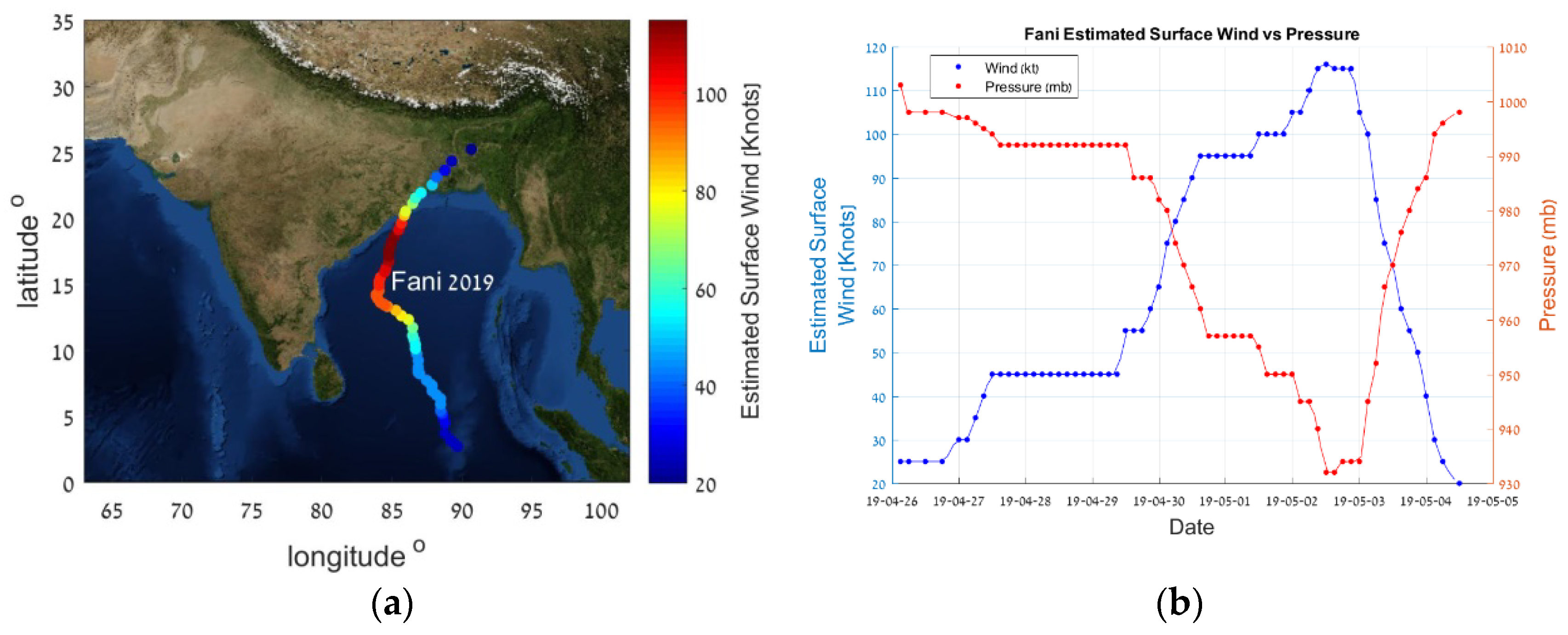
Extremely Severe Cyclonic Storm “Fani” originated from a low-pressure area that formed over the east Equatorial Indian Ocean and adjoining southeast Bay of Bengal in the early morning (0530 IST) of 25 April 2019 (Figure 1a). It developed into a well-marked low-pressure area over the same region on the same morning (0830 IST). Under favorable environmental conditions, Fani developed into a tropical depression over the same region by the following morning (0830 IST) of 26 April. Moving nearly northwestwards, it intensified the following day (27 April) into a deep depression over the same region in the early morning (0530 IST) and further into a cyclonic storm “Fani” around noon (1130 IST) of 27 April over the southeast Bay of Bengal and adjoining east Equatorial Indian Ocean. Fani then moved north-northwestwards and intensified into a severe cyclonic storm in the evening (1730 IST) of 29th over central parts of south Bay of Bengal. It then moved nearly northwards and further intensified into a very severe cyclonic storm in the early morning (0530 IST) of the 30th over the southwest Bay of Bengal. Climatologically, Fani was the most intense cyclonic storm crossing Odisha coast during the pre-monsoon season in the satellite era (since 1965). The development of the low pressure in the eye of the storm, together with the increase in the maximum sustained winds is shown in Figure 1b. The minimum pressure reached 932 hPa on 2 May 2019, with wind speeds reaching 116 knots.

A snapshot from the 3D animation of tropical cyclone Fani is shown in Figure 2a. The image shows the location of the eye of the storm (X) on the 2 May 2019 at 0200 IST during the maximum intensity of the storm. The dots represent the detected lightning activity in the previous 12 h (color-coded) showing the rain bands and the spiral structure of the convective regions in the tropical cyclone around the eye of the storm. The black/white shaded area represents the SH at 300 mb (hPa) (~9 km altitude) that also show the high concentrations of SH in the upper atmosphere near the eye of the storm, but the spiral structure of the storm can also clearly be seen in the SH data.

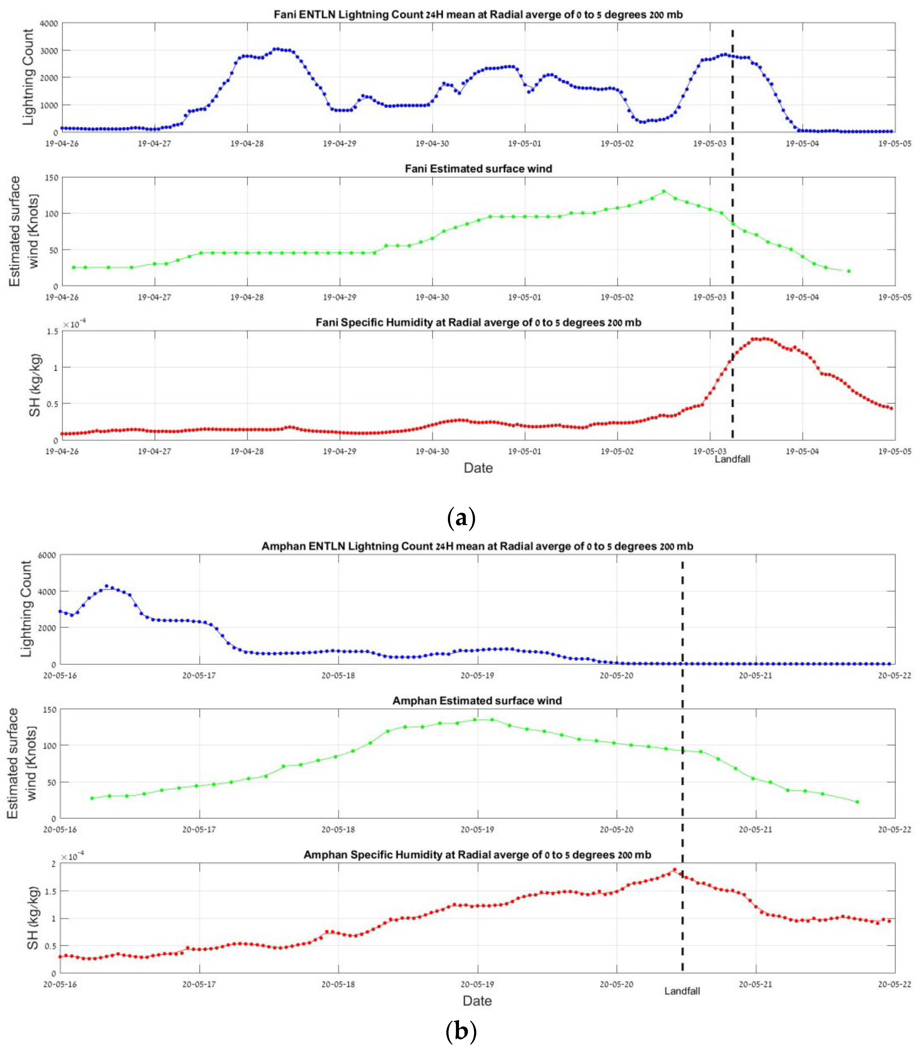
When we look at the time evolution of these three parameters (Figure 3a), we can see a clear lag between the development of each parameter in the storm. The lightning activity (blue curve) is the summation of all lightning strokes in a radius of 5 degrees from the center of the storm (~500 km radius), and peaks initially approximately 3 days before the maximum in SH in the upper troposphere, while the SH maximum occurs about 1 day after the maximum intensity of the tropical cyclone. The statistical correlation between the different parameters was performed using different pressure levels, and different spatial areas around the eye of the storm (1-degree radial radius from the eye or up to 5 degrees radial radius from the eye). The results of the correlation analysis are presented in

Table 1. Summary of 6 tropical cyclones listed in order of intensity from weakest to strongest. The intensity is represented by the minimum pressure or the maximum sustained winds around the eye of the storm. The Table shows the lag (in days) and the correlation coefficient between the time series of the maximum winds and the maximum SH at two levels (300 and 200 mb), after taking into account the lag between the two curves. The peak SH in the upper atmosphere (within a 5-degree radius of the eye) is also given in units of g/kg.

Cyclone Name	Min Pressure	Max Wind		SH 300 mb (~9 km)			SH 200 mb (~12 km)
	[mb]	[knots]	Lag after Min Pressure	r-Value	SH Max [g/kg]	Lag after Min Pressure	r-Value	SH Max [g/kg]
Titli	972 mb	80	+1 day	r = 0.93	0.55	+1 day	r = 0.57	0.09
Mekunu	960 mb	95	−1.25 day	r = 0.95	0.8	+1.5 days	r = 0.65	0.11
Idai	940 mb	115	+0.5 days	r = 0.8	0.85	+1.5 days	r = 0.88	1.1
Fani	932 mb	116	+2.5 days	r = 0.87	0.78	+1.5 days	r = 0.8	1.4
Amphan	901 mb	135	+1 day	r = 0.7	1.1	+1 day	r = 0.92	1.9
Mangkhut	897 mb	154	−1.5 days	r = 0.31	0.89	−1 day	r = 0.51	1.2

for the radial distance or 0–5 degrees.

For Fani the SH in the upper troposphere peaks between 1.5 and 2.5 days after the maximum intensity of the storm. When we compare the time series of wind speed and SH (taking into account the shift between the curves) the correlation coefficient is between r = 0.8–0.9 depending on the pressure level used for the SH (300 or 200 mb). The peak value of SH reaches 1.4 g/kg at the 200 mb level.

3.2. Tropical Cyclone Amphan (Category 5)

Amphan was a powerful and catastrophic tropical cyclone that caused widespread damage in Eastern India in May 2020. Causing over USD 13 billion of damage, Amphan is also the costliest cyclone ever recorded in the North Indian Ocean, surpassing the record held by Cyclone Nargis of 2008. The first tropical cyclone of the 2020 North Indian Ocean cyclone season, Amphan originated from a low-pressure area persisting 300 km east of Colombo, Sri Lanka, on 13 May 2020. Tracking northeastward, the disturbance organized over exceptionally warm sea surface temperatures. The Joint Typhoon Warning Center (JTWC) upgraded the system to a tropical depression on 15 May while the India Meteorological Department (IMD) followed suit the following day. On 17 May, Amphan underwent rapid intensification and became an extremely severe cyclonic storm within 12 h (Figure 4a).

On 18 May, at approximately 12:00 UTC, Amphan reached its peak intensity with 3-min sustained wind speeds of 130 knots, 1-min sustained wind speeds of 140 knots, and a minimum central barometric pressure of 920 mbar. The storm began an eyewall replacement cycle shortly after it reached its peak intensity, but the continued effects of dry air and wind shear disrupted this process and caused Amphan to gradually weaken as it paralleled the eastern coastline of India (Figure 4b). On 20 May, between 10:00 and 11:00 UTC, the cyclone made landfall in West Bengal. At the time, the JTWC estimated Amphan’s 1-min sustained winds to be 84 knots. Amphan rapidly weakened once inland and dissipated shortly thereafter. The development of the low pressure in the eye of the storm, together with the increase in the maximum sustained winds is shown in Figure 2b. The minimum pressure reached 920 hPa on 18 May 2020, with wind speeds reaching 140 knots.

A snapshot from the 3D animation of tropical cyclone Amphan is shown in Figure 2b The image shows the location of the eye of the storm (X) on the 18 May 2020 at 1200 UTC. The dots represent the detected lightning activity in the previous 12 h (color-coded) show the rain bands and the spiral structure of the convective regions in the tropical cyclone around the eye of the storm. The black-/white-shaded area represents the SH at 300 mb (hPa) that also shows the high concentrations in the upper atmosphere near the eye of the storm, but the spiral structure of the storm can also clearly be seen.

When we look at the time evolution of these three parameters (Figure 3b) we can see a clear lag between the development of each parameter in the storm. The lightning activity (blue curve) is the summation of all lightning strokes in a radius of 5 degrees from the center of the storm (~500 km radius), and peaks initially approximately 4 days before the maximum in SH in the upper troposphere, while the SH maximum occurs about 1 day after the maximum intensity of the tropical cyclone. The statistical correlation between the different parameters was performed using different pressure level, and different spatial areas around the eye of the storm (1-degree radial radius from the eye or up to 5 degrees radial radius from the eye). The results of the correlation analysis are presented in Table 1.

For Amphan the SH in the upper troposphere peaks 1 day after the maximum intensity of the storm. When we compare the time series of wind speed and SH (taking into account the shift between the curves) the correlation coefficient is between r = 0.7 and 0.92 depending on the pressure level used for the SH (300 or 200 mb). The peak value of SH reaches 1.9 g/kg at the 200 mb level.

3.3. Links between Storm Intensity and UTWV

We have so far analyzed six tropical storms in this study (Table 1) and when we look at the relationship between maximum storm intensity (either pressure or winds) and the amount of water vapor deposited in the upper troposphere, we see a strong linear relationship with stronger storms (lower minimum pressure) depositing more water vapor in the upper atmosphere (Figure 5). This should not be surprising, although the altitude of maximum deposition depends on the storm strength. Weaker storms tend to deposit more moisture at the lower 300 hPa level compared to the higher 200 hPa level, while the stronger storms transport more moisture aloft to the 200 hPa level. The linear regression curves give the sensitivity of upper tropospheric water vapor to changes in tropical storm intensity. From the linear regression curves, we see that for every 10 hPa decrease in minimum pressure in the eye of the tropical storms, there is a 0.21 g/kg increase in the amount of water vapor at the 200 hPa level in the upper troposphere above the storm.

Given that future predictions of increased greenhouse gases predict a large shift to more intense tropical storms [20], these results imply additional water vapor being transported and deposited in the upper troposphere as the climate warms, with all the implications associated with increasing UTWV.

4. Conclusions

In this study, we focused on the impact of tropical cyclones on the concentrations of water vapor in the upper troposphere. We used a number of data sets, including lightning data from the Earth Networks Total Lightning Network, tropical storm data of minimum pressure and maximum sustained winds speeds, and upper tropospheric SH data obtained from the ERA5 reanalysis product.

We have analyzed six tropical cyclones of different intensities to better understand the temporal evolution of these three parameters (lightning, wind speed and UTWV). While the link between lightning and wind speed has been published before [1], in this paper, we focus on the contribution of these monster storms on the upper tropospheric water vapor concentrations. The reason for focusing on UTWV is due to its importance in the climate system influencing the radiation balance of the planet. Furthermore, studies show that the intensity of tropical storms are likely to increase in the future, with less weak storms and more intense category 4 and 5 storms. Hence, the implications for UTWV are clear, and increasing the water vapor in the upper troposphere that is normally very dry, will act as a strong positive feedback to enhance any warming due to greenhouse gases alone. Our preliminary results (six storms) also show that the more intense the tropical cyclone, the higher in the atmosphere the water vapor is deposited (Table 1). This too is an important finding, since increasing the altitude of the water vapor in the upper troposphere also has major impacts on the radiation balance, even without changing the absolute amount of water vapor. The higher the water vapor is deposited, the larger the impact on Earth’s surface temperatures [4].

Our conceptual model to explain these relationships is as follows. The development and progression of tropical cyclones is accompanied with deep convective towers within the eyewalls of the storm, as well as in the rain bands. These deep convective cells can have significant updrafts that will result in large mixed-phase regions in the storms, allowing for the generation of electrification and lightning discharges. The strong updrafts that generate the lightning also transport vertically large amounts of water vapor, supercooled droplets, and ice crystals into the upper portions of the troposphere (~9–12 km). The outflow and divergence at the top of the tropical cyclones transport these hydrometeors away from the eye of the storm where they can evaporate/sublimate, resulting in the moistening of the upper troposphere above the TC. The transport of this humidity away from the eye of the storm takes time and, hence, lags behind the changes in the storm intensity (and lightning activity). Furthermore, as the storms increase in their intensity, the vertical transport of moisture increases, dumping more moisture in the upper troposphere.

This study has only analyzed six tropical storms, and hence more analysis is needed with more storms, and in other regions of the globe to further quantify this link with UTWV. It is also important to understand the contribution of tropical cyclones as a whole to the moistening of the upper atmosphere. Since tropical cyclones are seasonal in nature, and sporadic in time, there is a need to quantify their contribution the total concentrations of UTWV average of time and space.