
Regional Emissions Analysis of Light-Duty Battery Electric Vehicles


Abstract
:1. Introduction
2. Materials and Methods
2.1. Life-Cycle Analysis Modeling Framework
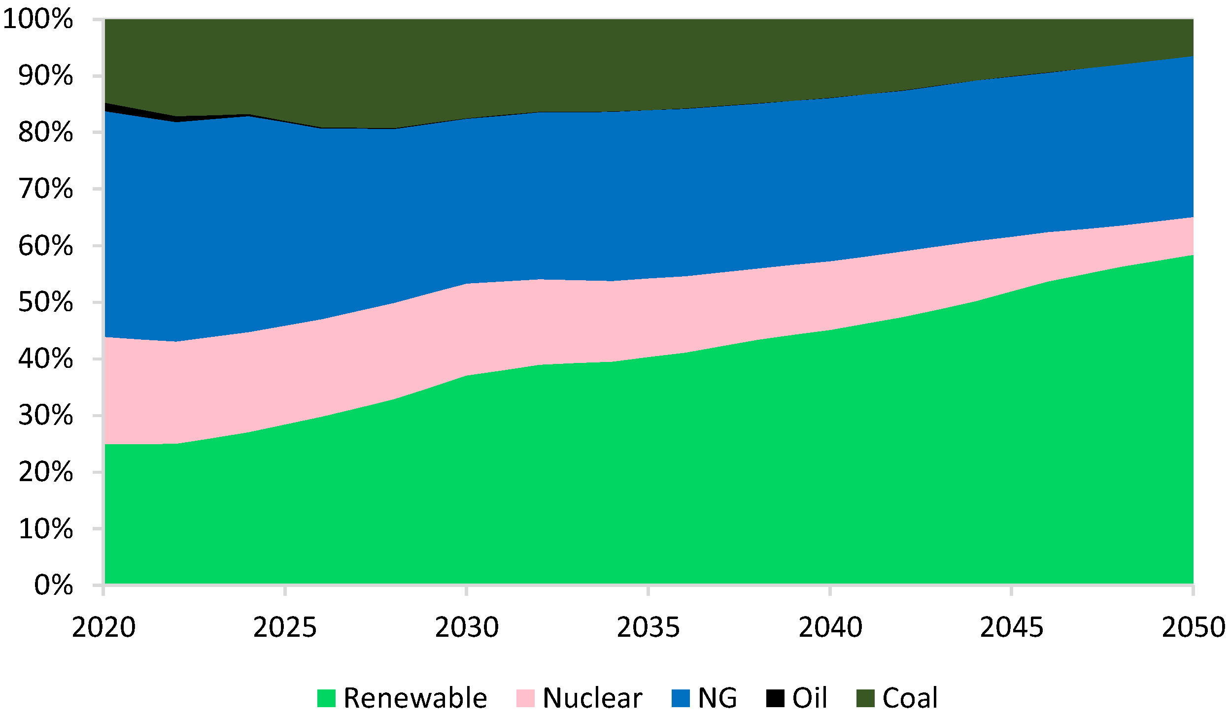
2.2. Electricity Grid Mix
2.3. Vehicle Operation Emission Factors
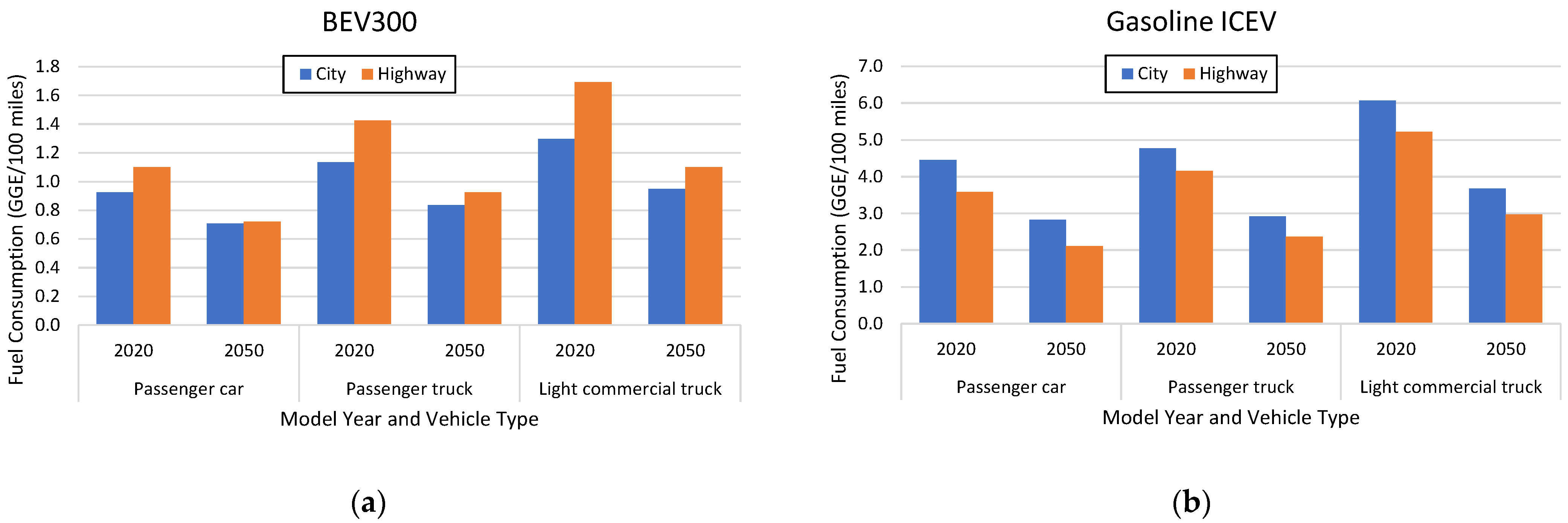
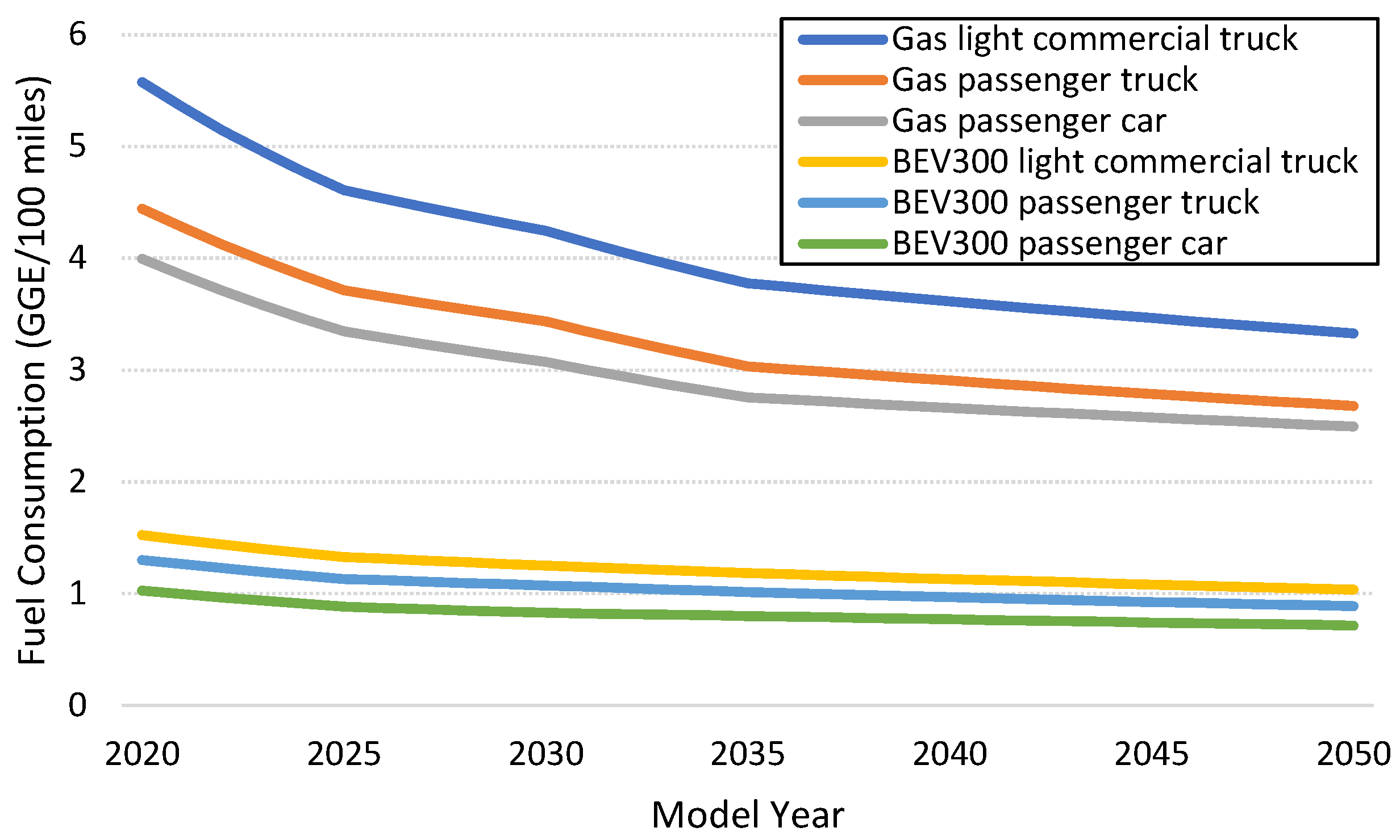
2.4. Vehicle Operation Fuel Consumption
2.4.1. Driving Patterns
2.4.2. Ambient Temperature
2.5. Vehicle-Cycle Assumptions
3. Results
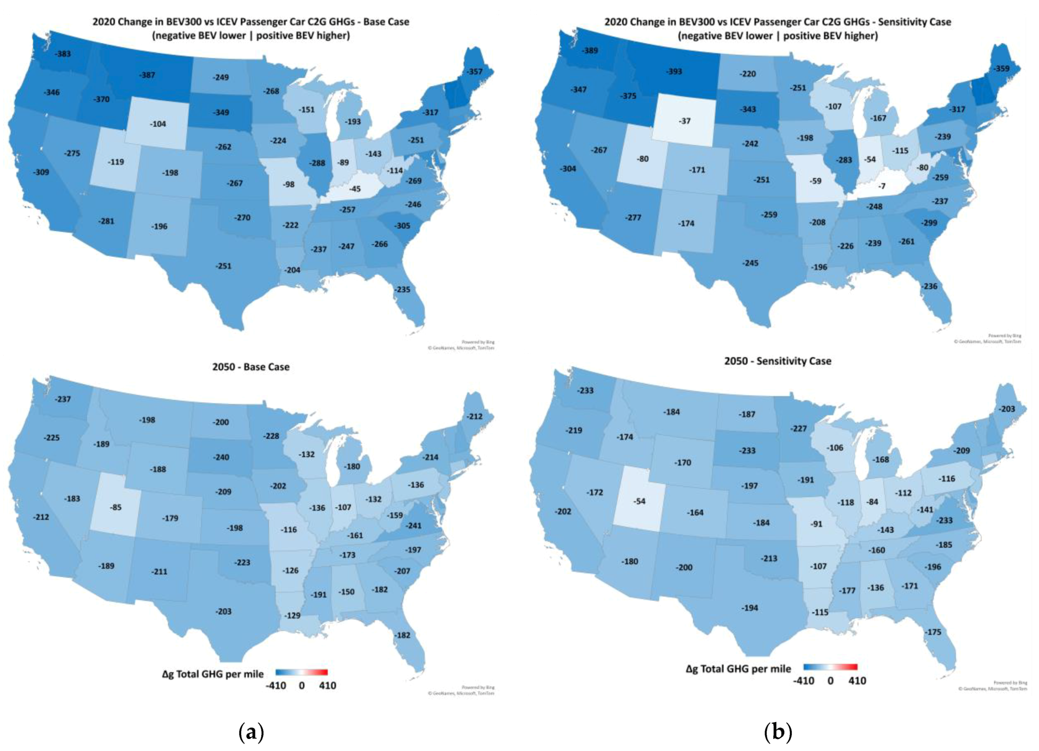
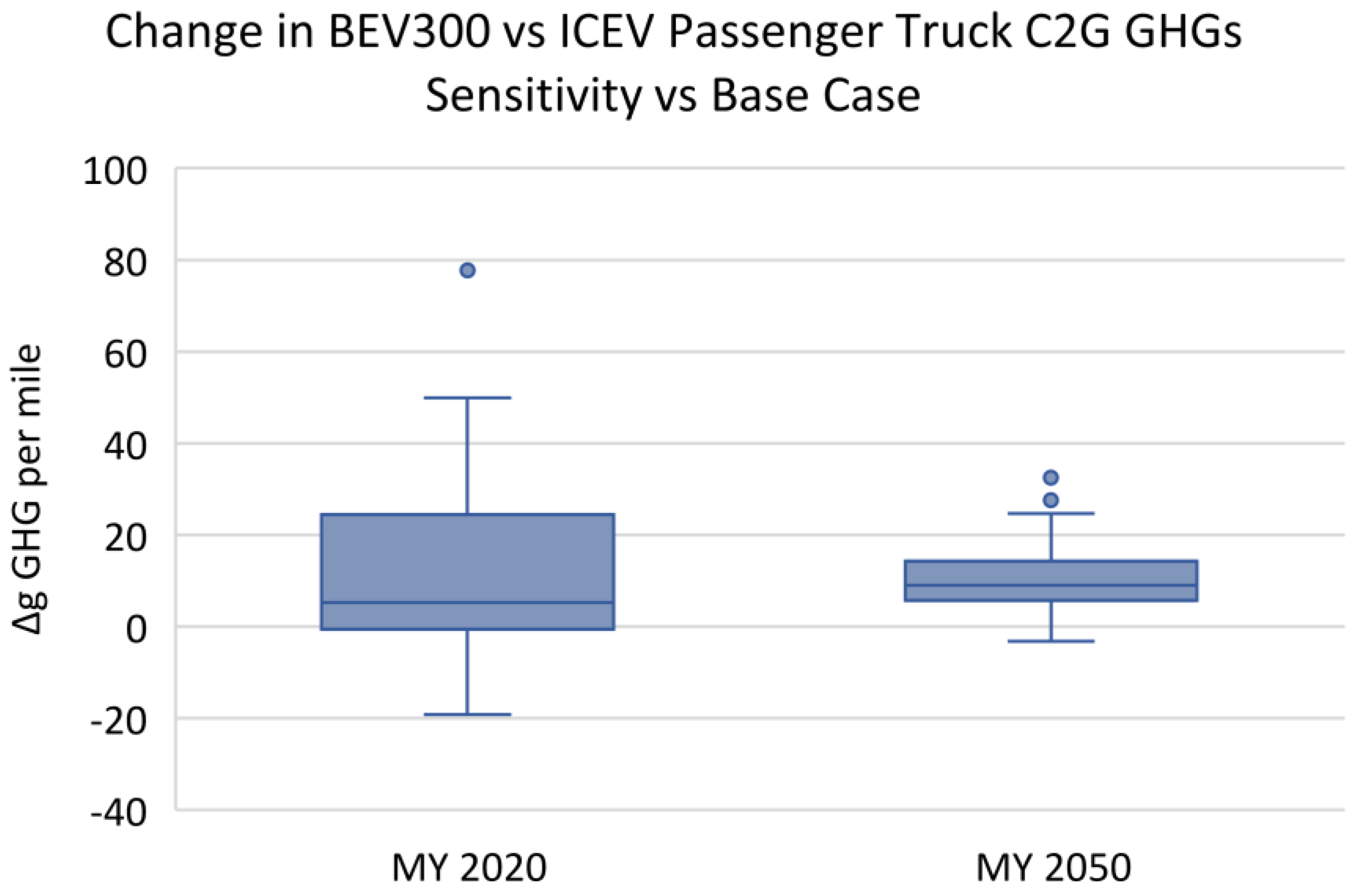
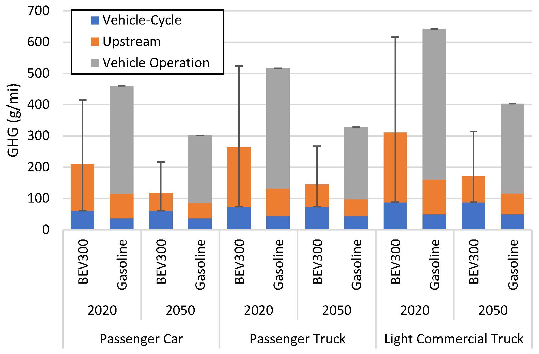
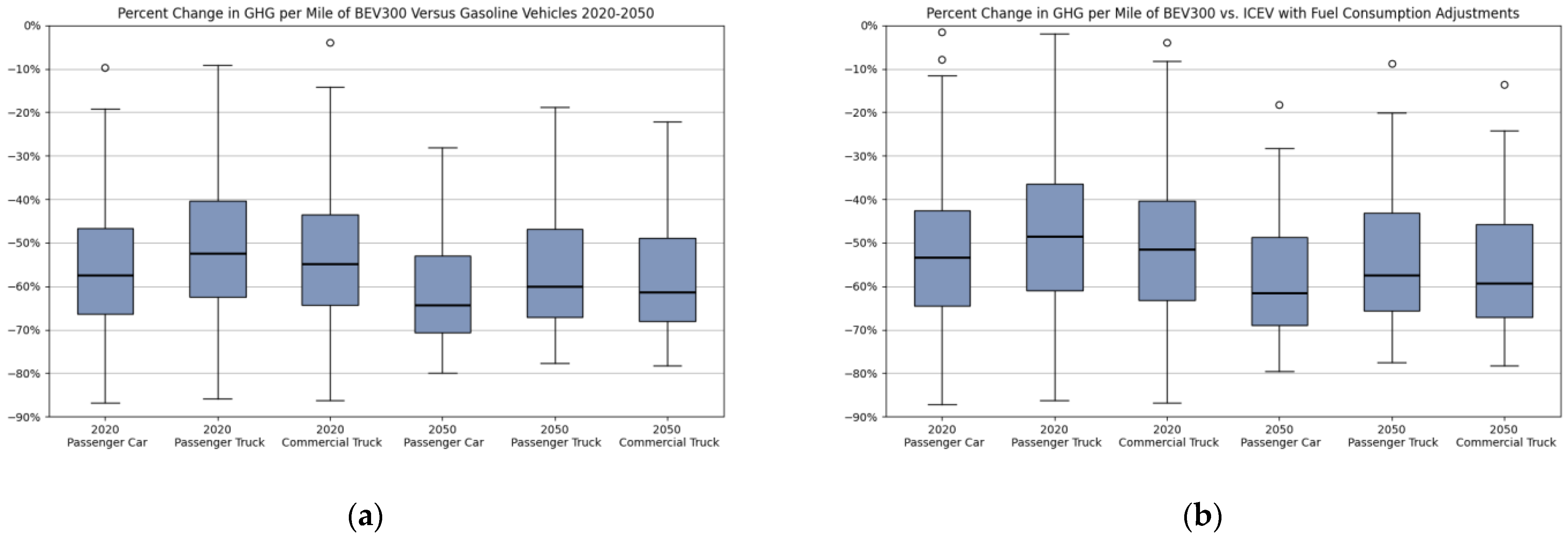
3.1. GHG Emissions
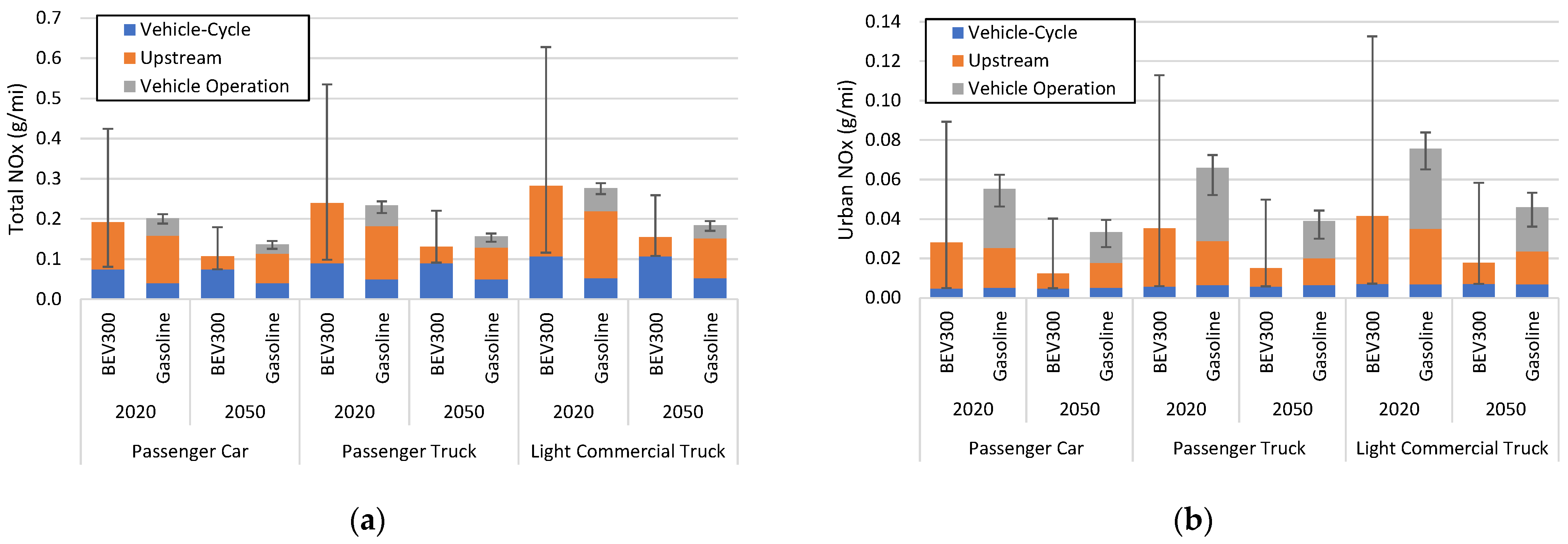
3.2. NOx and PM2.5 Emissions
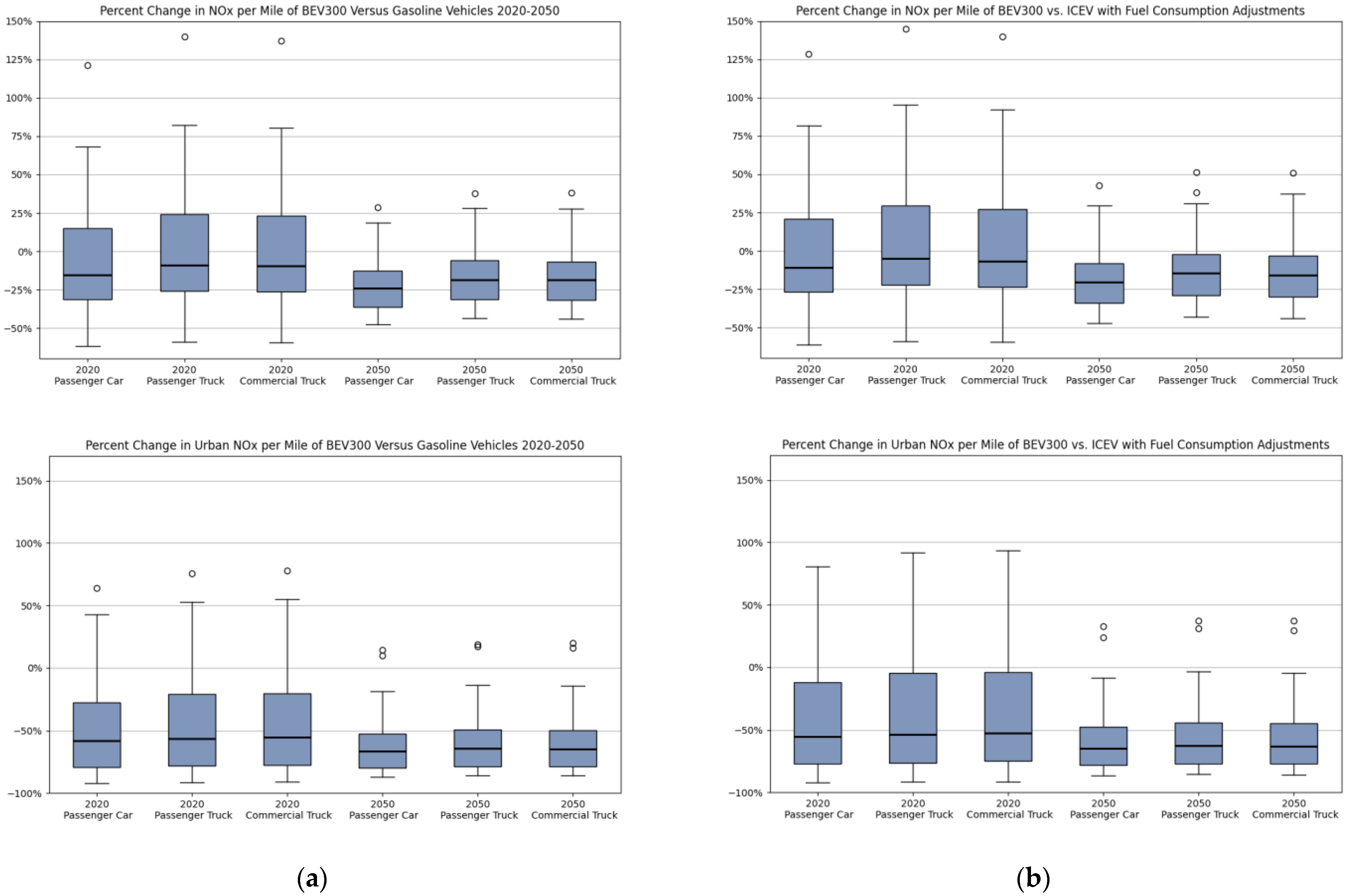
3.2.1. Total and Urban NOx
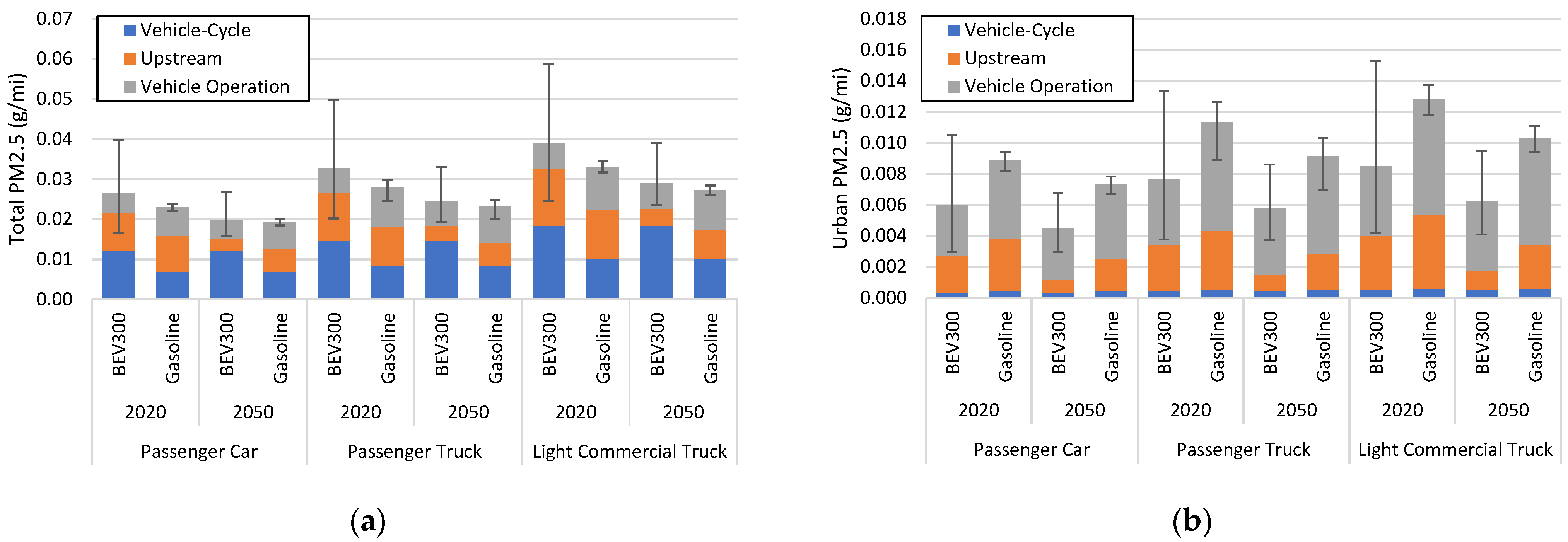
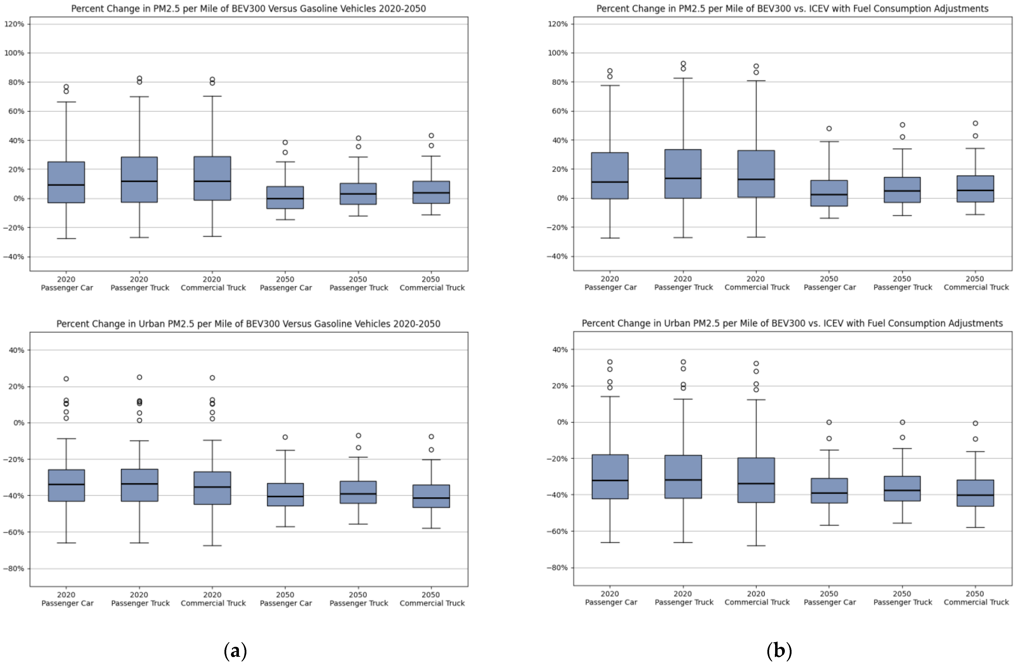
3.2.2. Total and Urban PM2.5
4. Discussion and Conclusions
Author Contributions
Funding
Institutional Review Board Statement
Informed Consent Statement
Data Availability Statement
Conflicts of Interest
Appendix A. State Generation Mixes

| State | 2020 Coal | 2020 Oil | 2020 NG | 2020 Renew | 2020 Nuclear | 2050 Coal | 2050 Oil | 2050 NG | 2050 Renew | 2050 Nuclear |
|---|---|---|---|---|---|---|---|---|---|---|
| Alabama | 11% | 2% | 50% | 6% | 31% | 13% | 0% | 39% | 13% | 35% |
| Arkansas | 15% | 3% | 52% | 6% | 25% | 21% | 0% | 39% | 15% | 25% |
| Arizona | 15% | 0% | 28% | 19% | 38% | 14% | 0% | 6% | 55% | 25% |
| California | 0% | 0% | 46% | 47% | 7% | 0% | 0% | 20% | 80% | 0% |
| Colorado | 33% | 0% | 30% | 37% | 0% | 18% | 0% | 5% | 77% | 0% |
| Connecticut | 0% | 0% | 49% | 11% | 40% | 0% | 0% | 66% | 34% | 0% |
| Delaware | 0% | 0% | 95% | 5% | 0% | 0% | 0% | 3% | 97% | 0% |
| Florida | 3% | 0% | 79% | 6% | 12% | 5% | 0% | 33% | 53% | 9% |
| Georgia | 9% | 0% | 50% | 12% | 29% | 3% | 0% | 38% | 36% | 23% |
| Iowa | 33% | 0% | 15% | 52% | 0% | 12% | 0% | 1% | 87% | 0% |
| Idaho | 0% | 0% | 16% | 84% | 0% | 0% | 0% | 39% | 61% | 0% |
| Illinois | 15% | 0% | 19% | 11% | 54% | 9% | 0% | 58% | 33% | 0% |
| Indiana | 53% | 3% | 33% | 12% | 0% | 25% | 0% | 43% | 32% | 0% |
| Kansas | 28% | 0% | 4% | 49% | 19% | 14% | 0% | 0% | 86% | 0% |
| Kentucky | 68% | 0% | 25% | 6% | 0% | 18% | 0% | 19% | 63% | 0% |
| Louisiana | 0% | 18% | 61% | 2% | 20% | 0% | 0% | 85% | 15% | 0% |
| Massachusetts | 0% | 0% | 55% | 45% | 0% | 0% | 0% | 17% | 83% | 0% |
| Maryland | 1% | 0% | 36% | 39% | 24% | 0% | 0% | 30% | 70% | 0% |
| Maine | 0% | 0% | 21% | 79% | 0% | 0% | 0% | 22% | 78% | 0% |
| Michigan | 32% | 4% | 22% | 14% | 28% | 2% | 0% | 40% | 47% | 11% |
| Minnesota | 22% | 0% | 17% | 41% | 19% | 3% | 0% | 1% | 80% | 15% |
| Missouri | 63% | 0% | 13% | 12% | 12% | 40% | 0% | 1% | 59% | 0% |
| Mississippi | 3% | 1% | 78% | 1% | 18% | 6% | 0% | 23% | 71% | 0% |
| Montana | 3% | 0% | 0% | 97% | 0% | 14% | 0% | 0% | 86% | 0% |
| North Carolina | 21% | 0% | 32% | 14% | 33% | 3% | 0% | 27% | 53% | 17% |
| North Dakota | 34% | 0% | 0% | 65% | 0% | 13% | 0% | 0% | 87% | 0% |
| Nebraska | 29% | 0% | 3% | 43% | 25% | 10% | 0% | 0% | 90% | 0% |
| New Hampshire | 0% | 0% | 2% | 26% | 72% | 0% | 0% | 1% | 56% | 43% |
| New Jersey | 0% | 0% | 59% | 8% | 33% | 0% | 0% | 61% | 39% | 0% |
| New Mexico | 32% | 2% | 29% | 37% | 0% | 6% | 0% | 8% | 86% | 0% |
| Nevada | 0% | 0% | 63% | 36% | 0% | 2% | 0% | 38% | 60% | 0% |
| New York | 1% | 2% | 36% | 38% | 22% | 0% | 0% | 21% | 79% | 0% |
| Ohio | 36% | 0% | 46% | 4% | 13% | 6% | 0% | 68% | 26% | 0% |
| Oklahoma | 3% | 6% | 48% | 44% | 0% | 4% | 0% | 5% | 91% | 0% |
| Oregon | 0% | 0% | 28% | 72% | 0% | 0% | 0% | 12% | 88% | 0% |
| Pennsylvania | 10% | 0% | 54% | 6% | 30% | 2% | 0% | 74% | 17% | 7% |
| Rhode Island | 0% | 0% | 68% | 32% | 0% | 0% | 0% | 12% | 88% | 0% |
| South Carolina | 12% | 0% | 21% | 13% | 54% | 3% | 0% | 17% | 60% | 19% |
| South Dakota | 5% | 0% | 15% | 80% | 0% | 0% | 0% | 1% | 99% | 0% |
| Tennessee | 23% | 0% | 22% | 13% | 42% | 0% | 0% | 51% | 21% | 28% |
| Texas | 5% | 5% | 52% | 30% | 9% | 5% | 0% | 16% | 74% | 5% |
| Utah | 50% | 0% | 33% | 18% | 0% | 43% | 0% | 18% | 39% | 0% |
| Virginia | 5% | 0% | 56% | 12% | 26% | 0% | 0% | 0% | 76% | 24% |
| Vermont | 0% | 0% | 0% | 100% | 0% | 0% | 0% | 20% | 80% | 0% |
| Washington | 0% | 0% | 9% | 84% | 7% | 0% | 0% | 3% | 97% | 0% |
| Wisconsin | 38% | 1% | 40% | 7% | 14% | 23% | 0% | 28% | 49% | 0% |
| West Virginia | 65% | 0% | 0% | 35% | 0% | 12% | 0% | 35% | 53% | 0% |
| Wyoming | 66% | 0% | 2% | 32% | 0% | 17% | 0% | 0% | 82% | 0% |
| U.S. Average | 15% | 1% | 40% | 25% | 19% | 6% | 0% | 28% | 58% | 7% |
Appendix B. Fuel Consumption
Appendix B.1. Driving Patterns
| State | Passenger Car (mph) | Passenger Truck (mph) | Light Commercial Truck (mph) | City% | Highway% |
|---|---|---|---|---|---|
| Alabama | 30.5 | 31.7 | 30.6 | 43% | 57% |
| Arizona | 29.8 | 30.7 | 30.0 | 44% | 56% |
| Arkansas | 32.0 | 33.2 | 32.0 | 40% | 60% |
| California | 30.7 | 31.2 | 30.8 | 43% | 57% |
| Colorado | 31.6 | 32.5 | 31.7 | 41% | 59% |
| Connecticut | 30.0 | 30.2 | 30.1 | 44% | 56% |
| Delaware | 28.5 | 29.3 | 28.6 | 47% | 53% |
| Florida | 27.9 | 28.5 | 28.0 | 48% | 52% |
| Georgia | 29.9 | 30.7 | 30.0 | 44% | 56% |
| Idaho | 33.2 | 34.6 | 33.1 | 38% | 62% |
| Illinois | 29.5 | 30.3 | 29.6 | 45% | 55% |
| Indiana | 30.6 | 31.7 | 30.7 | 43% | 57% |
| Iowa | 32.9 | 34.3 | 32.8 | 39% | 61% |
| Kansas | 33.6 | 34.9 | 33.6 | 37% | 63% |
| Kentucky | 32.8 | 34.1 | 32.8 | 39% | 61% |
| Louisiana | 30.7 | 31.7 | 30.7 | 43% | 57% |
| Maine | 33.6 | 34.9 | 33.4 | 37% | 63% |
| Maryland | 29.7 | 30.2 | 29.8 | 45% | 55% |
| Massachusetts | 28.3 | 28.5 | 28.5 | 48% | 52% |
| Michigan | 30.3 | 31.2 | 30.4 | 44% | 56% |
| Minnesota | 31.9 | 33.0 | 31.9 | 41% | 59% |
| Mississippi | 32.5 | 33.8 | 32.4 | 39% | 61% |
| Missouri | 33.9 | 34.9 | 33.8 | 37% | 63% |
| Montana | 35.3 | 36.7 | 35.1 | 34% | 66% |
| Nebraska | 34.1 | 35.5 | 34.0 | 36% | 64% |
| Nevada | 29.6 | 30.4 | 29.7 | 45% | 55% |
| New Hampshire | 31.6 | 32.6 | 31.6 | 41% | 59% |
| New Jersey | 28.6 | 28.8 | 28.7 | 47% | 53% |
| New Mexico | 32.0 | 33.4 | 32.0 | 40% | 60% |
| New York | 29.7 | 30.2 | 29.8 | 45% | 55% |
| North Carolina | 30.5 | 31.4 | 30.6 | 43% | 57% |
| North Dakota | 35.0 | 36.4 | 34.7 | 35% | 65% |
| Ohio | 31.0 | 31.9 | 31.1 | 42% | 58% |
| Oklahoma | 32.5 | 33.6 | 32.4 | 39% | 61% |
| Oregon | 31.0 | 32.1 | 31.0 | 42% | 58% |
| Pennsylvania | 30.3 | 31.2 | 30.4 | 44% | 56% |
| Rhode Island | 29.2 | 29.6 | 29.3 | 46% | 54% |
| South Carolina | 31.0 | 32.2 | 31.0 | 42% | 58% |
| South Dakota | 36.2 | 37.5 | 35.9 | 33% | 67% |
| Tennessee | 30.4 | 31.4 | 30.5 | 43% | 57% |
| Texas | 30.4 | 31.2 | 30.5 | 43% | 57% |
| Utah | 31.6 | 32.5 | 31.7 | 41% | 59% |
| Vermont | 34.6 | 35.8 | 34.3 | 36% | 64% |
| Virginia | 31.0 | 32.0 | 31.1 | 42% | 58% |
| Washington | 31.3 | 32.1 | 31.4 | 42% | 58% |
| West Virginia | 32.5 | 33.7 | 32.4 | 39% | 61% |
| Wisconsin | 32.5 | 33.7 | 32.4 | 39% | 61% |
| Wyoming | 35.7 | 37.2 | 35.5 | 33% | 67% |
| U.S. Average | 30.6 | 31.5 | 30.7 | 43% | 57% |
Appendix B.2. Ambient Temperature
| State | ICEV | BEV |
|---|---|---|
| Alabama | 1.018 | 1.052 |
| Arizona | 1.030 | 1.090 |
| Arkansas | 1.024 | 1.077 |
| California | 1.022 | 1.077 |
| Colorado | 1.052 | 1.198 |
| Connecticut | 1.041 | 1.154 |
| Delaware | 1.030 | 1.101 |
| Florida | 1.019 | 1.032 |
| Georgia | 1.017 | 1.047 |
| Idaho | 1.059 | 1.222 |
| Illinois | 1.040 | 1.147 |
| Indiana | 1.038 | 1.142 |
| Iowa | 1.051 | 1.192 |
| Kansas | 1.039 | 1.135 |
| Kentucky | 1.029 | 1.105 |
| Louisiana | 1.019 | 1.045 |
| Maine | 1.063 | 1.240 |
| Maryland | 1.031 | 1.107 |
| Massachusetts | 1.043 | 1.163 |
| Michigan | 1.056 | 1.211 |
| Minnesota | 1.070 | 1.266 |
| Mississippi | 1.019 | 1.052 |
| Missouri | 1.035 | 1.125 |
| Montana | 1.063 | 1.238 |
| Nebraska | 1.047 | 1.177 |
| Nevada | 1.039 | 1.148 |
| New Hampshire | 1.056 | 1.214 |
| New Jersey | 1.034 | 1.122 |
| New Mexico | 1.032 | 1.118 |
| New York | 1.051 | 1.193 |
| North Carolina | 1.021 | 1.070 |
| North Dakota | 1.071 | 1.267 |
| Ohio | 1.039 | 1.144 |
| Oklahoma | 1.030 | 1.093 |
| Oregon | 1.044 | 1.167 |
| Pennsylvania | 1.042 | 1.158 |
| Rhode Island | 1.038 | 1.143 |
| South Carolina | 1.018 | 1.051 |
| South Dakota | 1.058 | 1.218 |
| Tennessee | 1.025 | 1.086 |
| Texas | 1.024 | 1.059 |
| Utah | 1.046 | 1.173 |
| Vermont | 1.059 | 1.224 |
| Virginia | 1.027 | 1.097 |
| Washington | 1.046 | 1.172 |
| West Virginia | 1.034 | 1.126 |
| Wisconsin | 1.062 | 1.233 |
| Wyoming | 1.065 | 1.247 |
Appendix C. Additional Results

References
- Davis, S.; Boundy, R.G. Transportation Energy Data Book, 39th ed.; ORNL/TM-2020/1770 United States 10.2172/1767864 ORNL English; Oak Ridge National Lab. (ORNL): Oak Ridge, TN, USA, 2021. [Google Scholar]
- EPA. Inventory of U.S. Greenhouse Gas Emissions and Sinks 1990–2019; EPA 430-R-21-005; Environmental Protection Agency: Washington, DC, USA, 2021.
- EPA. 2017 National Emissions Inventory (NEI) Data; United States Environmental Protection Agency: Washington, DC, USA, 2021.
- Cai, H.; Wang, M.; Elgowainy, A.; Han, J. Life-Cycle Greenhouse Gas and Criteria Air Pollutant Emissions of Electric Vehicles in the United States. SAE Int. J. Altern. Powertrains 2013, 2, 325–336. [Google Scholar] [CrossRef]
- Tessum, C.W.; Hill, J.D.; Marshall, J.D. Life cycle air quality impacts of conventional and alternative light-duty transportation in the United States. Proc. Natl. Acad. Sci. USA 2014, 111, 18490–18495. [Google Scholar] [CrossRef] [PubMed] [Green Version]
- Holland, S.P.; Mansur, E.T.; Muller, N.Z.; Yates, A.J. Are There Environmental Benefits from Driving Electric Vehicles? The Importance of Local Factors. Am. Econ. Rev. 2016, 106, 3700–3729. [Google Scholar] [CrossRef] [Green Version]
- Yuksel, T.; Tamayao, M.-A.M.; Hendrickson, C.; Azevedo, I.M.L.; Michalek, J.J. Effect of regional grid mix, driving patterns and climate on the comparative carbon footprint of gasoline and plug-in electric vehicles in the United States. Environ. Res. Lett. 2016, 11, 044007. [Google Scholar] [CrossRef]
- Wu, D.; Guo, F.; Field, F.R.; De Kleine, R.D.; Kim, H.C.; Wallington, T.J.; Kirchain, R.E. Regional Heterogeneity in the Emissions Benefits of Electrified and Lightweighted Light-Duty Vehicles. Environ. Sci. Technol. 2019, 53, 10560–10570. [Google Scholar] [CrossRef] [PubMed] [Green Version]
- Requia, W.J.; Mohamed, M.; Higgins, C.D.; Arain, A.; Ferguson, M. How clean are electric vehicles? Evidence-based review of the effects of electric mobility on air pollutants, greenhouse gas emissions and human health. Atmos. Environ. 2018, 185, 64–77. [Google Scholar] [CrossRef]
- Brugge, D.; Durant, J.L.; Rioux, C. Near-highway pollutants in motor vehicle exhaust: A review of epidemiologic evidence of cardiac and pulmonary health risks. Environ. Health 2007, 6, 23. [Google Scholar] [CrossRef] [PubMed] [Green Version]
- Wang, M.; Elgowainy, A.; Han, J.; Benavides, P.T.; Burnham, A.; Cai, H.; Canter, C.; Chen, R.; Dai, Q.; Kelly, J.; et al. Summary of Expansions, Updates, and Results in GREET 2017 Suite of Models; Argonne National Lab. (ANL): Argonne, IL, USA, 2017; 28p. [Google Scholar]
- Wang, M.; Elgowainy, A.; Benavides, P.T.; Burnham, A.; Cai, H.; Dai, Q.; Hawkins, T.R.; Kelly, J.C.; Kwon, H.; Lee, D.-Y.; et al. Summary of Expansions and Updates in GREET® 2018; Argonne National Lab. (ANL): Argonne, IL, USA, 2018; 32p. [Google Scholar]
- Wang, M.; Elgowainy, A.; Lee, U.; Benavides, P.T.; Burnham, A.; Cai, H.; Dai, Q.; Hawkins, T.R.; Kelly, J.; Kwon, H.; et al. Summary of Expansions and Updates in GREET® 2019; Argonne National Lab. (ANL): Argonne, IL, USA, 2019. [Google Scholar]
- Wang, M.; Elgowainy, A.; Lee, U.; Bafana, A.; Benavides, P.T.; Burnham, A.; Cai, H.; Dai, Q.; Gracida-Alvarez, U.R.; Hawkins, T.R.; et al. Summary of Expansions and Updates in GREET® 2020; ANL/ESD-20/9; 163298 United States; 163298 ANL English; Argonne National Lab. (ANL): Argonne, IL, USA, 2020; 35p. [Google Scholar] [CrossRef]
- EIA. Electricity Explained: Electricity Generation, Capacity, and Sales in the United States. Available online: https://www.eia.gov/energyexplained/electricity/electricity-in-the-us-generation-capacity-and-sales.php (accessed on 6 September 2021).
- Ray, S. New Electric Generating Capacity in 2020 Will Come Primarily from Wind and Solar. Available online: https://www.eia.gov/todayinenergy/detail.php?id=42495 (accessed on 6 September 2021).
- Ray, S. Renewables Account for Most New U.S. Electricity Generating Capacity in 2021. Available online: https://www.eia.gov/todayinenergy/detail.php?id=46416 (accessed on 6 September 2021).
- DieselNet. United States: Light-Duty Vehicles: GHG Emissions & Fuel Economy. Available online: https://dieselnet.com/standards/us/fe_ghg.php (accessed on 14 September 2021).
- DieselNet. United States: New Engine and Vehicle Emissions: Cars and Light-Duty Trucks. Available online: https://dieselnet.com/standards/us/ld.php (accessed on 14 September 2021).
- Preston, B. The Coming Wave of Electric SUVs and Pickup Trucks. Consumer Reports, 18 February 2021. Available online: https://www.consumerreports.org/hybrids-evs/the-coming-wave-of-electric-suvs-and-pickup-trucks-a8170180441/(accessed on 14 September 2021).
- Pachauri, R.K.; Allen, M.R.; Barros, V.R.; Broome, J.; Cramer, W.; Christ, R.; Church, J.A.; Clarke, L.; Dahe, Q.; Dasgupta, P. Climate Change 2014: Synthesis Report. Contribution of Working Groups I, II and III to the Fifth Assessment Report of the Intergovernmental Panel on Climate Change; IPCC: Geneva, Switzerland, 2014. [Google Scholar]
- Huo, H.; Wu, Y.; Wang, M. Total versus urban: Well-to-wheels assessment of criteria pollutant emissions from various vehicle/fuel systems. Atmos. Environ. 2009, 43, 1796–1804. [Google Scholar] [CrossRef]
- Cole, W.; Gagnon, P.; Corcoran, S.; Das, P.; Frazier, W.; Gates, N.; Hale, E.; Mai, T. 2020 Standard Scenarios Report: A U.S. Electricity Sector Outlook; National Renewable Energy Lab. (NREL): Golden, CO, USA, 2021.
- EPA. Motor Vehicle Emission Simulator (MOVES3.0.1); United States Environmental Protection Agency: Washington, DC, USA, 2021.
- EPA. Exhaust Emission Rates for Light-Duty Onroad Vehicles in MOVES3; EPA-420-R-20-019; United States Environmental Protection Agency: Washington, DC, USA, 2020.
- Islam, E.S.; Moawad, A.; Kim, N.; Rousseau, A. Energy Consumption and Cost Reduction of Future Light-Duty Vehicles through Advanced Vehicle Technologies: A Modeling Simulation Study Through 2050; ANL/ESD-19/10; 161542 United States; 161542 ANL English; Argonne National Lab. (ANL): Argonne, IL, USA, 2020; 45p. [Google Scholar] [CrossRef]
- Elgowainy, A.; Burnham, A.; Wang, M.; Molburg, J.; Rousseau, A.; Systems, E. Well-to-Wheels Energy Use and Greenhouse Gas Emissions Analysis of Plug-In Hybrid Electric Vehicles; ANL/ESD/09-2; TRN: US200911%%458 United States; TRN: US200911%%458 ANL English; Argonne National Lab. (ANL): Argonne, IL, USA, 2009. [Google Scholar] [CrossRef] [Green Version]
- Elgowainy, A.; Han, J.; Poch, L.; Wang, M.; Vyas, A.; Mahalik, M.; Rousseau, A. Well-to-Wheels Analysis of Energy Use and Greenhouse Gas Emissions of Plug-In Hybrid Electric Vehicles; Argonne National Lab. (ANL): Argonne, IL, USA, 2010. [Google Scholar]
- Final Technical Support Document; United States EPA.OoT., Air Quality, Standards Division, Innovative: New York, NY, USA, 2006.
- Santos, A.; McGuckin, N.; Nakamoto, H.Y.; Gray, D.; Liss, S. Summary of Travel Trends: 2017 National Household Travel Survey; Federal Highway Administration: Washington, DC, USA, 2018. Available online: https://www.ncdc.noaa.gov/cag/ (accessed on 21 October 2021).
- Lohse-Busch, H.; Duoba, M.; Rask, E.; Stutenberg, K.; Gowri, V.; Slezak, L.; Anderson, D. Ambient Temperature (20 °F, 72 °F and 95 °F) Impact on Fuel and Energy Consumption for Several Conventional Vehicles, Hybrid and Plug-In Hybrid Electric Vehicles and Battery Electric Vehicle. In SAE Technical Paper; Society of Automotive Engineers: Warrendale, PA, USA, 2013. [Google Scholar] [CrossRef]
- Burnham, A.; Wang, M.Q.; Wu, Y. Development and applications of GREET 2.7—The Transportation Vehicle-CycleModel; ANL/ESD/06-5; TRN: US0701918 United States; TRN: US0701918 available ANL ENGLISH; Argonne National Lab. (ANL): Argonne, IL, USA, 2006. [Google Scholar] [CrossRef] [Green Version]
- Dai, Q.; Kelly, J.C.; Gaines, L.; Wang, M. Life Cycle Analysis of Lithium-Ion Batteries for Automotive Applications. Batteries 2019, 5, 48. [Google Scholar] [CrossRef] [Green Version]
- Burnham, A.; Gohlke, D.; Rush, L.; Stephens, T.; Zhou, Y.; Delucchi, M.A.; Birky, A.; Hunter, C.; Lin, Z.; Ou, S.; et al. Comprehensive Total Cost of Ownership Quantification for Vehicles with Different Size Classes and Powertrains; ANL/ESD-21/4; 167399 United States; 167399 ANL English; Argonne National Lab. (ANL): Argonne, IL, USA, 2021; 225p. [Google Scholar] [CrossRef]
- House, T.W. FACT SHEET: President Biden Sets 2030 Greenhouse Gas Pollution Reduction Target Aimed at Creating Good-Paying Union Jobs and Securing U.S. Leadership on Clean Energy Technologies. Available online: https://www.whitehouse.gov/briefing-room/statements-releases/2021/04/22/fact-sheet-president-biden-sets-2030-greenhouse-gas-pollution-reduction-target-aimed-at-creating-good-paying-union-jobs-and-securing-u-s-leadership-on-clean-energy-technologies/ (accessed on 22 September 2021).
- National Academies of Sciences, Engineering and Medicine. Deployment of Deep Decarbonization Technologies: Proceedings of a Workshop; The National Academies Press: Washington, DC, USA, 2019; p. 126. [Google Scholar]
- Gan, Y.; Lu, Z.; He, X.; Hao, C.; Wang, Y.; Cai, H.; Wang, M.; Elgowainy, A.; Przesmitzki, S.; Bouchard, J. Provincial Greenhouse Gas Emissions of Gasoline and Plug-in Electric Vehicles in China: Comparison from the Consumption-Based Electricity Perspective. Environ. Sci. Technol. 2021, 55, 6944–6956. [Google Scholar] [CrossRef] [PubMed]
- NOAA. Climate at a Glance: Statewide Mapping; NOAA: Silver Spring, MD, USA, 2021.

Publisher’s Note: MDPI stays neutral with regard to jurisdictional claims in published maps and institutional affiliations. |
© 2021 by the authors. Licensee MDPI, Basel, Switzerland. This article is an open access article distributed under the terms and conditions of the Creative Commons Attribution (CC BY) license (https://creativecommons.org/licenses/by/4.0/).
Share and Cite
Burnham, A.; Lu, Z.; Wang, M.; Elgowainy, A. Regional Emissions Analysis of Light-Duty Battery Electric Vehicles. Atmosphere 2021, 12, 1482. https://doi.org/10.3390/atmos12111482
Burnham A, Lu Z, Wang M, Elgowainy A. Regional Emissions Analysis of Light-Duty Battery Electric Vehicles. Atmosphere. 2021; 12(11):1482. https://doi.org/10.3390/atmos12111482
Chicago/Turabian StyleBurnham, Andrew, Zifeng Lu, Michael Wang, and Amgad Elgowainy. 2021. "Regional Emissions Analysis of Light-Duty Battery Electric Vehicles" Atmosphere 12, no. 11: 1482. https://doi.org/10.3390/atmos12111482
APA StyleBurnham, A., Lu, Z., Wang, M., & Elgowainy, A. (2021). Regional Emissions Analysis of Light-Duty Battery Electric Vehicles. Atmosphere, 12(11), 1482. https://doi.org/10.3390/atmos12111482