Numerical Modeling of Ozone Loss in the Exceptional Arctic Stratosphere Winter–Spring of 2020

Abstract

Dynamical processes and changes in the ozone layer in the Arctic stratosphere during the winter of 2019–2020 were analyzed using numerical experiments with a chemistry-transport model (CTM) and reanalysis data. The results of numerical calculations using CTM with Dynamic parameters specified from the Modern Era Retrospective analysis for Research and Applications, version 2 (MERRA-2) reanalysis data, carried out according to several scenarios of accounting for the chemical destruction of ozone, demonstrated that both Dynamic and chemical processes contribute significantly to ozone changes over the selected World Ozone and Ultraviolet Radiation Data Centre network stations, both in the Eastern and in the Western hemispheres. Based on numerical experiments with the CTM, the specific Dynamic conditions of winter–spring 2019–2020 described a decrease in ozone up to 100 Dobson Units (DU) in the Eastern Hemisphere and over 150 DU in the Western Hemisphere. In this case, the photochemical destruction of ozone in both the Western and Eastern Hemispheres at a maximum was about 50 DU with peaks in April in the Eastern Hemisphere and in March and April in the Western Hemisphere. Heterogeneous activation of halogen gases on the surface of polar stratospheric clouds, on the one hand, led to a sharp increase in the destruction of ozone in chlorine and bromine catalytic cycles, and, on the other hand, decreased its destruction in nitrogen catalytic cycles. Analysis of wave activity using 3D Plumb fluxes showed that the enhancement of upward wave activity propagation in the middle of March over the Gulf of Alaska was observed during the development stage of the minor sudden stratospheric warming (SSW) event that led to displacement of the stratospheric polar vortex to the north of Canada and decrease of polar stratospheric clouds’ volume.

1. Introduction

The circulation of the Arctic stratosphere in the winter-spring season (hereinafter, winter season) is characterized by strong interannual and seasonal variability [1], which can affect the tropospheric circulation and weather conditions (e.g., [2,3,4,5,6]), and the temperature and chemical composition of the stratosphere, upper atmosphere (e.g., [7,8]), and ozone layer (e.g., [9,10]). Due to the strong wave activity and the frequent occurrence of SSW events, and, consequently, the unstable and warm stratospheric polar vortex, significant ozone anomalies are observed in the Arctic less often than in the Antarctic, where a major SSW event was observed only in September 2002 [11].

Prior to the 2019–2020 winter season, the large ozone depletion was observed in the Arctic stratosphere in the spring of 1996 [12], 1997 [13], 2000 [14], 2005 [15], and the largest one in 2011 [16,17]. A possibly even greater ozone reduction in the Arctic stratosphere in the 2015–2016 winter season compared to 2010–2011 was prevented by a SSW event in March 2016 [18,19]. Nevertheless, in January–February 2016, lower values of the total column ozone (up to ~200 Dobson Units (DU)) were observed in the northern part of Russia, which was 50% less than the average climatic values [20]. Analysis of the model simulation revealed that these anomalies were mainly due to Dynamic reasons [21].

The 2019–2020 winter season in the Arctic stratosphere was characterized by an extremely strong, stable, and exceptionally long-lived stratospheric polar vortex (e.g., [22,23,24]). It was caused by reduced wave activity propagation from the troposphere into the stratosphere and its downward reflection from the upper stratosphere, which strengthened the polar vortex through residual circulation changes [22]. In late February–early March 2020, record low temperatures in the Arctic lower stratosphere resulted in a record volume of Polar Stratospheric Clouds (PSCs) [22,25]. As a result of the prevailing meteorological conditions favorable for ozone depletion, during 5 weeks in March and April 2020, the values of the total column ozone were less than 220 DU, which allowed speaking about the first such long-term ozone anomaly in the Arctic [26]. For the first time in all the years of observations, the analysis of data from a number of selected ozonesondes revealed an extremely strong decrease in the ozone content in the Arctic stratosphere in the spring of 2020, amounting to up to 90% [25]. According to simulations of chemistry and transport model ATLAS [27], very low ozone values inside the Arctic polar vortex in the lower stratosphere were caused by exceptionally long periods in the history of these air masses with low temperatures in sunlight.

Microwave Limb Sounder (MLS) satellite data [28] also indicated record low ozone concentrations in the polar stratosphere during the Arctic 2020 spring, which began to be recorded earlier than in all other years and ended later than in all other years, with the exception of the winter season 2010–2011 [23]. According to data produced by the Copernicus Atmosphere Monitoring service (CAMS reanalysis) the monthly mean ozone columns in the Arctic in March 2020 were up to 180 DU or 40% lower than mean values over 2003–2019 (CAMS climatology) while values for 2011 and 1997 were lower by 31% and 35%, respectively [29]. Severe ozone depletion led to a large increase of solar ultraviolet radiation, according to measurements performed at 10 Arctic and subarctic locations between early March and mid-April 2020 [30]. According to OMPS LP satellite observations, the area of the PSCs in the winter 2019–2020 in the Arctic reached the values typical for Antarctic conditions [31]. The major conclusion of these studies is that the reason for such record strong ozone depletion in the spring 2020 was an unusually cold and isolated stratospheric polar vortex. Analysis of TOMCAT/SLIMCAT chemistry transport model simulations [32] demonstrated that very low ozone observed in the Arctic stratosphere in March 2020 was caused mainly by anomalously weak wintertime Dynamic replenishment.

Model experiments indicated that one of the reasons for the low wave activity propagation to the stratosphere could be the positive phase of the dipole in the Indian Ocean (IOD), defined as the SST gradient between the western and eastern equatorial Pacific Ocean. The positive phase of IOD through the propagation of wave chains to the northeast led to a weakening of the Aleutian low [33], which, by analogy with the El Niño-South Oscillation effect, weakens the propagation of planetary waves from the troposphere to the stratosphere [34]. The frequency of positive IOD events doubled in the 20th century and their intensity increased, and, according to model projections, this trend is expected to continue [35].

According to model estimations taking into account the decrease in the content of ozone-depleting substances since the early 2000s and the continued growth of greenhouse gases, significant ozone layer anomalies comparable to record depletion in spring 2011 could be observed in the Arctic by the middle of this century [36]. It has been suggested that, due to changes in the stratospheric climate, the cold northern winters will get colder in the coming decades and it will influence the winter loss of Arctic ozone (e.g., [28,37,38]). The cooling of the stratosphere could delay the recovery of the ozone layer [39]. A significant impact of climate change on stratospheric ozone recovery is expected after the year 2050 but simultaneously could lead to an increase of UV-B irradiance by +1.3% per decade [40]. The other results of model simulations showed that climate change will accelerate stratospheric ozone recovery instead of delaying it (e.g., [36]).

Assessing the role of climate change in the occurrence of winter seasons with significant depletion of the ozone layer in the stratosphere, both in the Arctic and in the Antarctic, remains an urgent task, which determines the timing of ozone layer recovery [10,39]. By the end of the 20th century, the increasing anthropogenic impact on the ozone layer led to the formation of a tendency towards a decrease in the thickness of the ozone layer on a global scale and the regular appearance of spring ozone holes in Antarctica and the episodic appearance of large ozone holes in the Arctic. The unprecedented measures taken by the joint efforts in the framework of the Montreal protocol to reduce emissions of ozone-depleting substances containing chlorine and bromine components have led to a decrease in the tendency for an increase in the content of ozone-depleting substances in the stratosphere [41], and in recent years there have been signs of recovery of the ozone content [10,17]. However, for most data sets and regions the total ozone trends since the stratospheric halogen reached its maximum (in 1996–2000) are mostly not significantly different from zero (e.g., [42,43]).

In most studies of the variability of the Arctic stratospheric ozone, the main attention was focused on its evolution inside the polar vortex during its entire existence, taking into account the trajectory of the vortex movement (can be considered as the Lagrangian approach). Meanwhile, the change in the ozone content in selected geographic points, periodically located either inside the polar vortex or outside it (Euler’s approach), is also of interest. In this work, in particular, considerable attention was paid to the Euler approach for the selected four stations, at which ground-based measurements of the ozone content are carried out, the results of which, when they become available, can be compared with the results of satellite observations and model calculations.

On the other hand, when assessing the chemical destruction of ozone inside a polar vortex, changes in its gas-phase destruction that arise due to the transition of nitrogen radicals into the liquid and solid phases during the formation of PSCs and interaction of nitrogen and halogen compounds are most often not considered. In this study, we quantitatively evaluated not only the destruction of ozone in halogen catalytic cycles, which occurs as a result of heterogeneous processes on the surface of the PSCs, but also a decrease in its destruction in nitrogen catalytic cycles as a result of a decrease in the content of nitrogen radicals.

Our investigation focused on the following interesting issues of the exceptional Arctic winter season 2019–2020 that, as for our knowledge, were not discussed early:

-

Calculations with the chemistry transport model with Dynamic parameters specified from the MERRA-2 reanalysis data, carried out according to several scenarios of accounting for the chemical destruction of ozone, and

-

Dynamic processes contributed to the onset of the minor SSW event in late March 2020.

The paper is organized in the following manner. The data used and diagnostic methods are described in Section 2. Diagnostic results of the ozone layer and Dynamic evolution for the Northern Hemisphere stratosphere winter of 2019–2020 are given in Section 3. Results of chemistry-transport modeling experiments performed to determine the relative role of Dynamic and chemical processes in the formation of the Arctic ozone anomaly in the spring 2020 are presented in Section 4. The discussion and conclusions are given in Section 5.

2. Materials and Methods

The present study of the Dynamic and chemical processes and variability of the ozone layer in the Arctic stratosphere was carried out using numerical modeling with the Russian State Hydrometeorological University chemistry-transport model (RSHU CTM) [44], reanalysis data of National Centers for Environmental Prediction (NCEP) [45], MERRA-2 [46], and observational data. A brief description of applied methods of analysis is presented below.

The evolution of a minimum lower stratosphere temperature averaged over the polar cap in the winter of 2019–2020 and temperature anomalies of stratosphere–troposphere relative to climate means over 1981–2010 were analyzed using NCEP Reanalysis data. The propagation of wave activity was analyzed by using the zonal mean meridional heat flux and three-dimensional Plumb flux [47] calculated using NCEP Reanalysis data. It is known as an extended Eliassen–Palm (EP) flux due to the fact that its zonal average is equal to the well-known EP flux. The Plumb flux vectors are proportional to the group velocity of a planetary wave packet indicating the direction of propagation of the wave activity and are useful to localize regions of wave activity sources and sinks.

In diagnostic studies, a Plumb flux vectors were employed for different time scales from climatological studies of wave activity of 10 years (e.g., [47]) down to several days (e.g., [48]). In the present study, 3-day means were used in the calculation of the Plumb flux vectors.

The influence of the circulation of the Arctic stratosphere on the troposphere was analyzed through the propagation from the stratosphere to the troposphere of geopotential height anomalies from climatic values in the region of 60–90° N, normalized to the standard deviation (σ). When multiplied by −1, this parameter corresponds to the North Annular Mode (NAM) index. Following [49], the periods with an uninterrupted downward propagation of NAM index with values above ±1.5 σ from the middle stratosphere to troposphere were defined as events with a consistent downward propagation of anomalies to the troposphere. Notably, that zonal–mean eddy heat flux, which is a proxy for the upward wave activity propagation, averaged over prior 40 days, was highly anti-correlated (−0.8) with the NAM index at 10 hPa [50].

To assess the relative role of chemical and dynamic processes in the ozone anomalies’ formation, numerical experiments with a chemical transport model were carried out. The temporal evolution of the Arctic stratospheric gases was simulated with the RSHU CTM using meteorological fields directly from the reanalysis data [44]. This version of the global RSHU CTM is based on the Institute of Numerical Mathematics and RSHU chemistry-climate model (INM RAS—RSHU CCM) [51,52]. Meteorological fields were specified from Modern-Era Retrospective Analysis for Research and Applications version 2 (MERRA-2) reanalysis [46]. The RSHU CTM has a 5 degrees × 4 degrees horizontal resolution in longitude by latitude and 31 vertical sigma levels from the surface up to approximately 60 km. The model includes 74 oxygen, hydrogen, nitrogen, chlorine, bromine, carbon, and sulfate species. The chemistry of the species was calculated as described in [53]. Polar Stratospheric Clouds’ (PSCs’) formation and evolution were treated as a NAT, STS (super cooled ternary solution) (H₂O/HNO₃/H₂SO₄), based on the parameterization described in [54], and ice. PSCs’ surface variability, depending on temperature, pressure, and partial pressures of the relevant gases, including denitrification and dehydration through sedimentation was taken into account according to [55,56].

Calculations using the CTM were performed for 1 year from 1 July 2019 to 30 June 2020. The initial conditions for the initialization of the model were taken from historical calculations using the chemistry-climate model of the INM RAS—RSHU [51] for the period from 1979 to 2019. In historical calculations, at the lower boundary of the model, the mixing ratios of ozone-depleting substances were set based on the WMO2018 scenarios [39] and greenhouse gases based on the 5th IPCC report [57].

Numerical experiments with the RSHU CTM for two additional scenarios to the baseline (PSC) scenario were done. The first scenario (noPSC) did not include the formation of PSCs during the Arctic winter and spring (from 1 December to 15 May north to 60°N), while the second scenario did not include any chemical ozone destruction (noCHEM) in this area during the same period. Due to the fact that in the upper stratosphere it is difficult to correctly simulate ozone variability without considering chemical reactions [27], in the noCHEM scenario, chemistry was turned off only at altitudes below 10 mb (about 32 km).Comparison of the baseline scenario with these two additional scenarios allowed estimating the periods when the chemical destruction of ozone is most effective after heterogeneous activation on the PSC surface. In addition, based on a comparison of these calculation scenarios, it was possible to assess the comparative role of Dynamic and chemical processes of ozone reduction.

Total column ozone (TCO) data at the selected observational stations measured by the Ozone Monitoring Instrument (OMI) instrument onboard the AURA satellite [58] were used for comparison with results of model simulations. Additionally, Solar Backscatter Ultraviolet Version (SBUV) total ozone climatological data [59] averaged over the period of 1979–2019 were employed because they cover a longer period than OMI data.

3. Results

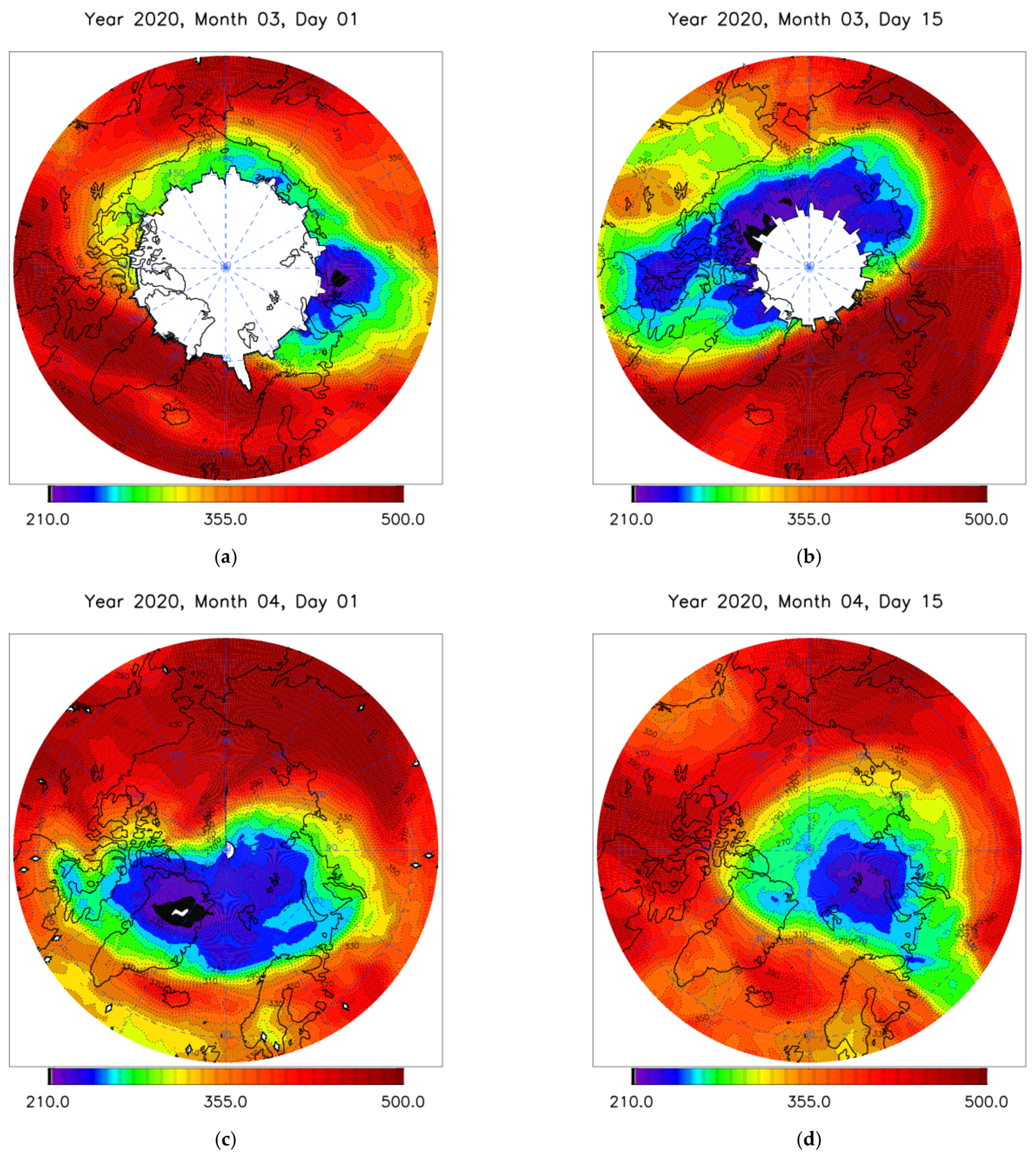
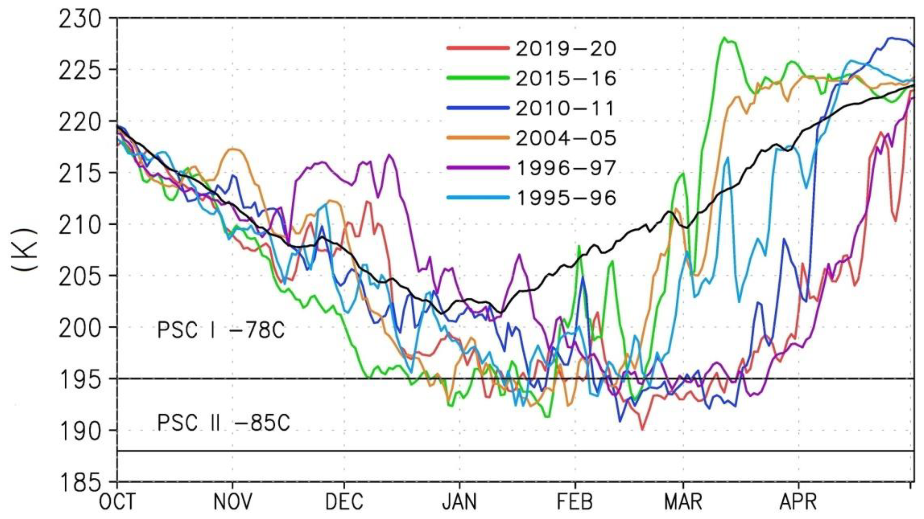
3.1. Main Features of Arctic Stratosphere Winter 2019–2020

The evolution of the total column ozone (TCO) in the Arctic in March–April 2020 as measured by the OMI instrument is presented in Figure 1. Measurements indicated that the ozone anomaly in early March (Figure 1a) covered mainly the Eastern part of the Arctic with minimum values less than 220 DU in the Northern part of the European territory of Russia. In the Western Arctic, values below 300 DU were observed north of Alaska and Western Canada. A significant part of the Arctic was still in the polar night region at the beginning of March and was not covered by the measurements of the OMI instrument, which uses solar radiation. On the other hand, in the absence of the Sun, the chemical destruction of ozone did not yet reach the high values associated with the previous halogen activation on the surface of polar stratospheric clouds; therefore, it can be assumed, that there should not be extremely low values of TCO in the region of absence of observations by the OMI instrument.

In mid-March (Figure 1b), the ozone anomaly turned around the pole to the East, covering most of the Arctic region of the Western Hemisphere with minimum values less than 220 DU in the area of Northern Greenland and the Canadian Arctic Archipelago north to the Canadian mainland. Again, the minimum values were detected along the border of the region of absence of observations—the zone of polar night. In the Eastern Hemisphere, values below 250 DU were found north of the mainland of Eastern Siberia. By the beginning of April (Figure 1c), the ozone anomaly turned further eastward, shifting towards Greenland, the Norwegian Sea, Svalbard, and Franz Josef Land. The minimum values of less than 200 DU were observed in the Northern part of Greenland. By mid-April, the ozone anomaly continued to move eastwards, covering most of the Arctic region of the Eastern Hemisphere with minimum values less than 220 DU in the Franz Josef Land archipelago. At the same time, the area with values below 300 DU also covered a significant part of Northwest Russia.

The winter season of 2019–2020 in the Arctic stratosphere was one of the coldest in the last 60 years (e.g., [22,25]). The minimum temperatures of the lower stratosphere since mid-February were either the lowest or close to the record lowest observed in the winter season of 2010–2011, and sufficient (with temperatures below 195 K) for the formation of PSC type 1 (Nitric Acid Trihydrate (NAT) particles) (Figure 2). Negative temperature anomalies, relative to climatic values over the period of 1981–2010, were observed in the polar lower stratosphere during almost the entire winter season of 2019–2020 with maximum values in the range from −15 K to −10 K from mid-February to mid-April. Two main causes of such cold and stable Arctic polar vortex were suggested. First, reduced upward wave activity propagation from the troposphere to the stratosphere resulted in lower stratosphere temperature [60]; second, downward refraction of wave activity from the upper stratosphere [22]. The evolution of wave activity propagation during the winter of 2019–2020 is illustrated by the variability of the zonal mean meridional heat flux (Figure 3a). Reduced upward wave activity propagation was observed mainly over two periods: from about 5 to 20 January and from 7 February to 7 March. The latter period was followed by enhanced wave activity propagation over about 10 days in the middle of March.

The daily integrated zonal mean heat flux values in the lower stratosphere at 70 hPa over three time periods in the winter of 2019–2020 and the other five winters with strong and cold stratospheric polar vortex and severe ozone destruction, 1995–1996, 1996–1997, 2004–2005, 2010–2011, and 2015–2016, were compared (Figure 3b). These integrated zonal mean values were normalized by the number of days in each period. The first period (7 February–7 March) was characterized by the largest and lasted a month, weakening the upward wave activity propagation in the winter of 2019–2020. The second and third periods were selected as January–February and January–March. It was seen that heat fluxes in the first and second periods were the lowest in 2020 and in the third period only slightly stronger than in 1997.

At the same time, the winter season of 2019–2020 in most of Northern Eurasia was characterized by anomalously warm weather due to increased westerly winds. A record high February monthly mean temperature was achieved in Siberia. Positive temperature anomalies over Northern Eurasia of more than 5 K were obtained when averaged over January–March 2020 [22]. The period with strongly reduced wave activity was characterized by positive anomalies of temperature over northeastern Eurasia (Figure 3c). The positive anomalies, up to 6–8 K, were observed over the Northeastern Eurasia during the period of strongly reduced upward wave activity propagation: 7 February–7 March.

The dominant mode of circulation in the troposphere of boreal extratropical latitudes is the Arctic Oscillation (AO). The AO positive phase is characterized by a reduced pressure at the pole and increased pressure in the region of 40–50° N [61]. With a positive AO phase, a stronger western zonal transport leads to milder winters, but with more precipitation in Southern Europe. In the negative AO phase, this transfer is weaker; as a result, cold air masses from the Arctic spread more strongly to the territory of Eurasia. Interaction between the dynamics of the stratosphere and the troposphere can cause changes in the AO. The strong and weak stratospheric polar vortex is often accompanied by a positive and negative AO phase, respectively [61].

In the first half of January and February–March 2020, a positive AO phase was observed with index values of more than 4 in early January and then in February–March. Average monthly values of the AO index were 3.4 in February and 2.6 in March. Thus, the positive AO phase with a reduced propagation of wave activity into the stratosphere could contribute to the enhancement of the Arctic stratospheric polar vortex [22].

Further to investigate the influence of the circulation of the Arctic stratosphere on the troposphere, the changes of the NAM index were analyzed. In the second half of February and during most of March 2020, areas with NAM index values above 1.5 standard deviation (σ) continuously propagated downward from the middle stratosphere to the lower troposphere, which indicated the influence of the Arctic stratosphere on the troposphere (Figure 4). This downward propagation was observed until late March 2020.

We assumed that the anomalously warm winter 2019–2000 in the extratropical troposphere (and especially from early February until early March with high positive AO index) contributed to the strengthening of the stratospheric polar vortex due to a decrease in the propagation of wave activity into the stratosphere from the troposphere. It is known that the main source of wave activity propagation into the stratosphere, characterized by the maximum of the vertical component Fz of Plumb’s fluxes, was located over the north-eastern Eurasia (e.g., [62,63,64]). Comparison of the two diagrams with Plumb vertical component Fz at 100 hPa averaged over 7 February–7 March 2020 (Figure 5a) and corresponding climate mean over 1981–2010 (Figure 5b) showed that the weakening of the upward wave activity propagation in the first period was observed from Scandinavia eastward over northeastern Eurasia. We assumed that this weakened upward propagation of wave activity could be associated with positive temperature anomalies over northeastern Eurasia. On the other hand, a strong stratospheric polar vortex in February–March 2020 influenced the high latitude troposphere, enhancing the positive AO phase.

After the period with a strongly weakened propagation of wave activity from the troposphere to the stratosphere (from early February until early March), a sharp increase in such propagation was observed in the upper troposphere–lower stratosphere over northwestern Canada in the middle of March over about 10 days. This can be seen in Figure 5c, showing the vertical component of the Plumb fluxes in the lower stratosphere at 100 hPa during the development stage of the SSW event on 14–16 March. The enhanced propagation of wave activity, which led to the minor SSW event, was apparently associated with the Rossby wave-breaking event in the troposphere over the Gulf of Alaska region (150–120° W) and was accompanied by a poleward transport of wet and warm air masses with low potential vorticity and formation of an anticyclone (Figure 5d). Daily ERA5 potential vorticity maps at the lower stratosphere from 13 to 18 March 2020 also displayed this Rossby wave-breaking event. Such a poleward transport, leading through a change in the zonal current and redirection of wave activity upward to the stratosphere (instead of the equator), can lead to the development of a SSW event, as in January 2006 [65].

Propagation of wave activity in the middle of March was analyzed using Plumb fluxes (Figure 6). On 11–13 March, altitude–latitudinal diagram of Plumb fluxes showed pronounced equatorward propagation of wave activity in the upper troposphere–lower stratosphere (Figure 6a). Later on, the enhanced upward propagation of wave activity in the troposphere and lower-middle stratosphere was clearly seen on 14–16 March (Figure 6c). Zonal mean zonal wind weakening in the lower–middle stratosphere over high latitudes was also observed. An altitude–longitude diagram of Plumb fluxes over the high latitudes (50–70° N) illustrated enhanced upward and eastward propagation from the region of an anticyclone formed in the troposphere over the Gulf of Alaska–northwestern Canada, nearby 160–140° W (Figure 6d). On a similar diagram 3 days earlier (11–13 March), such enhanced wave activity propagation and the anticyclone over the same region was not observed (Figure 6b). Enhanced upward wave activity propagation in the lower stratosphere over the region of the Gulf of Alaska–northwestern Canada was observed until 24–25 March.

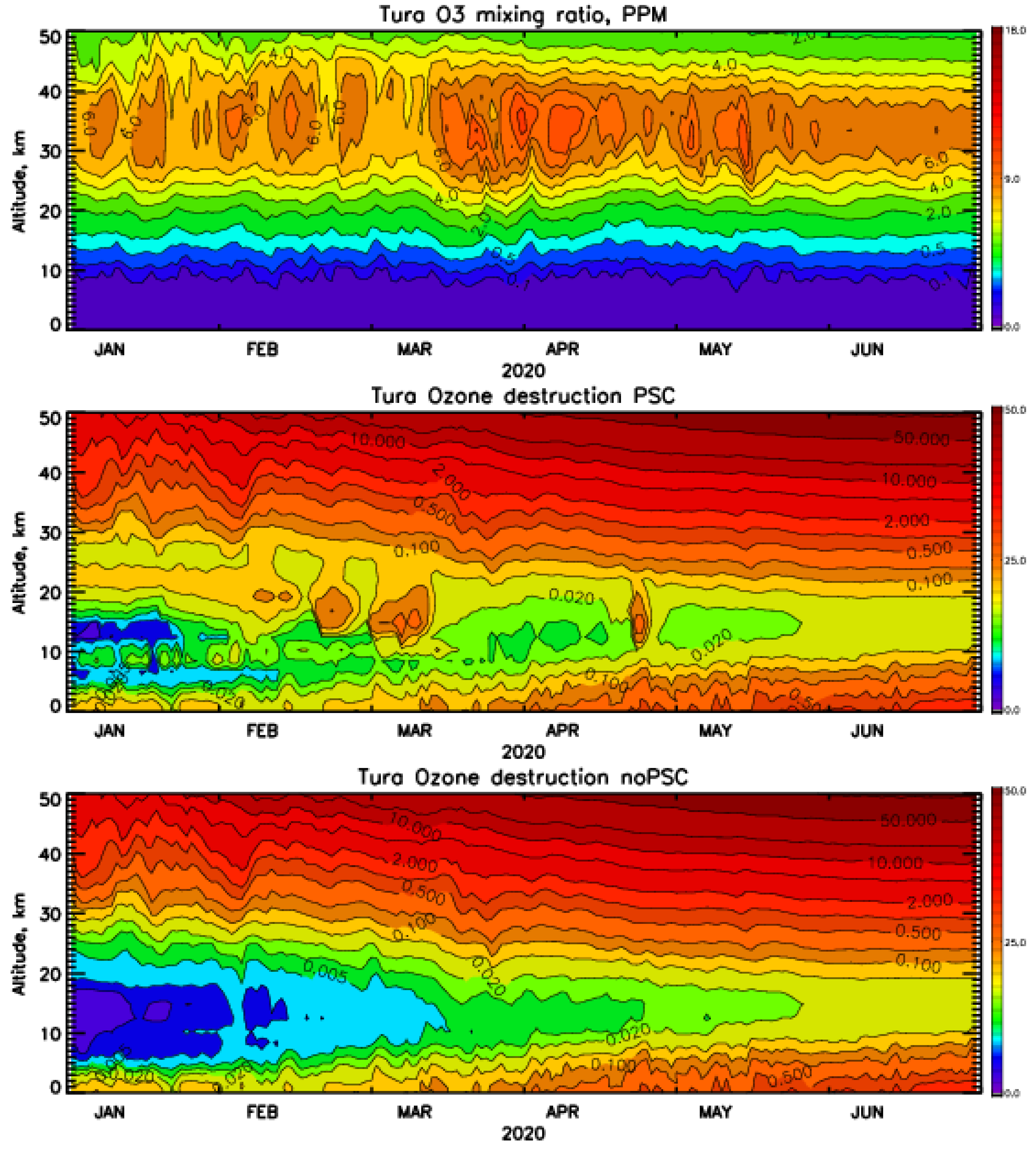
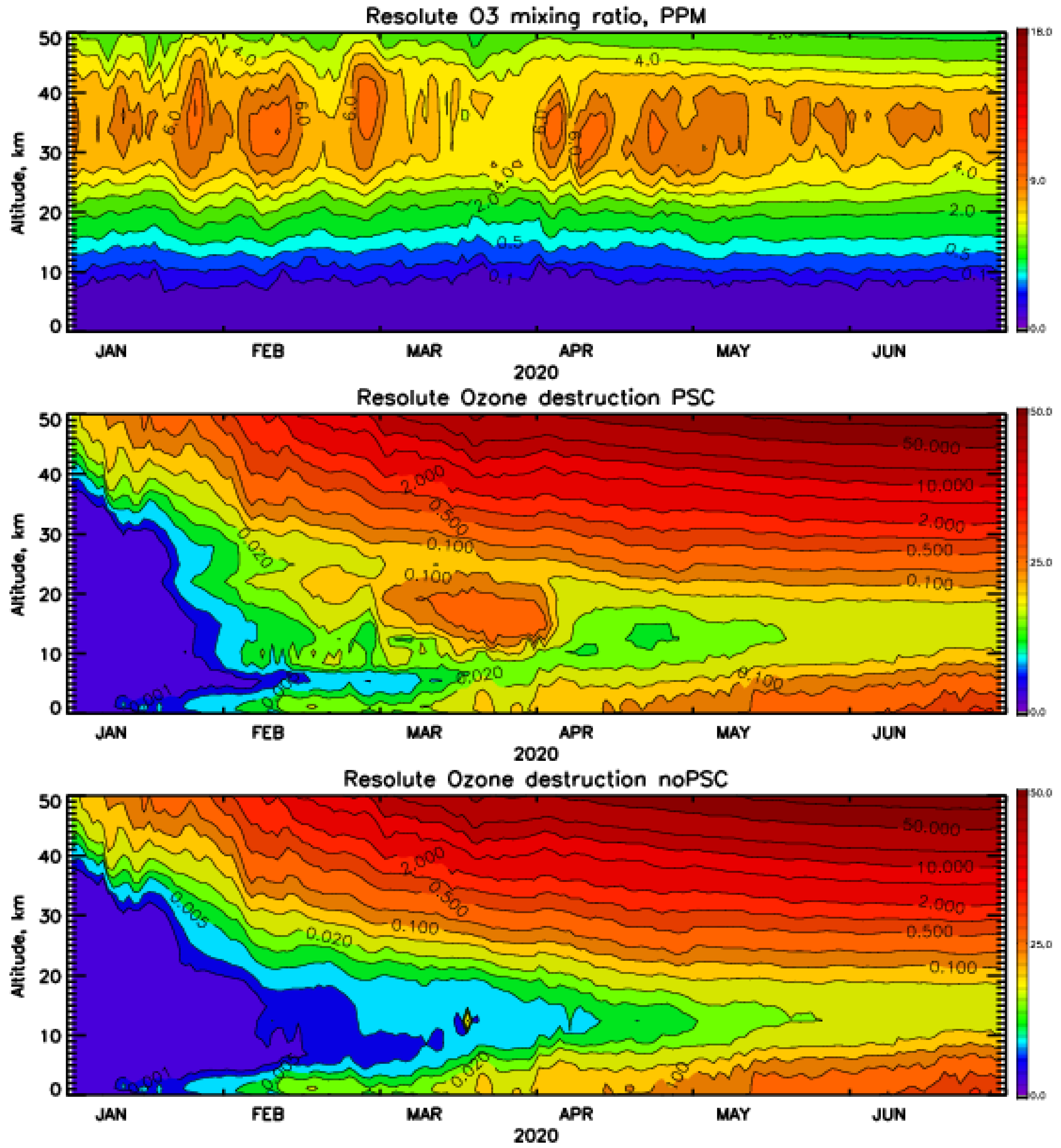
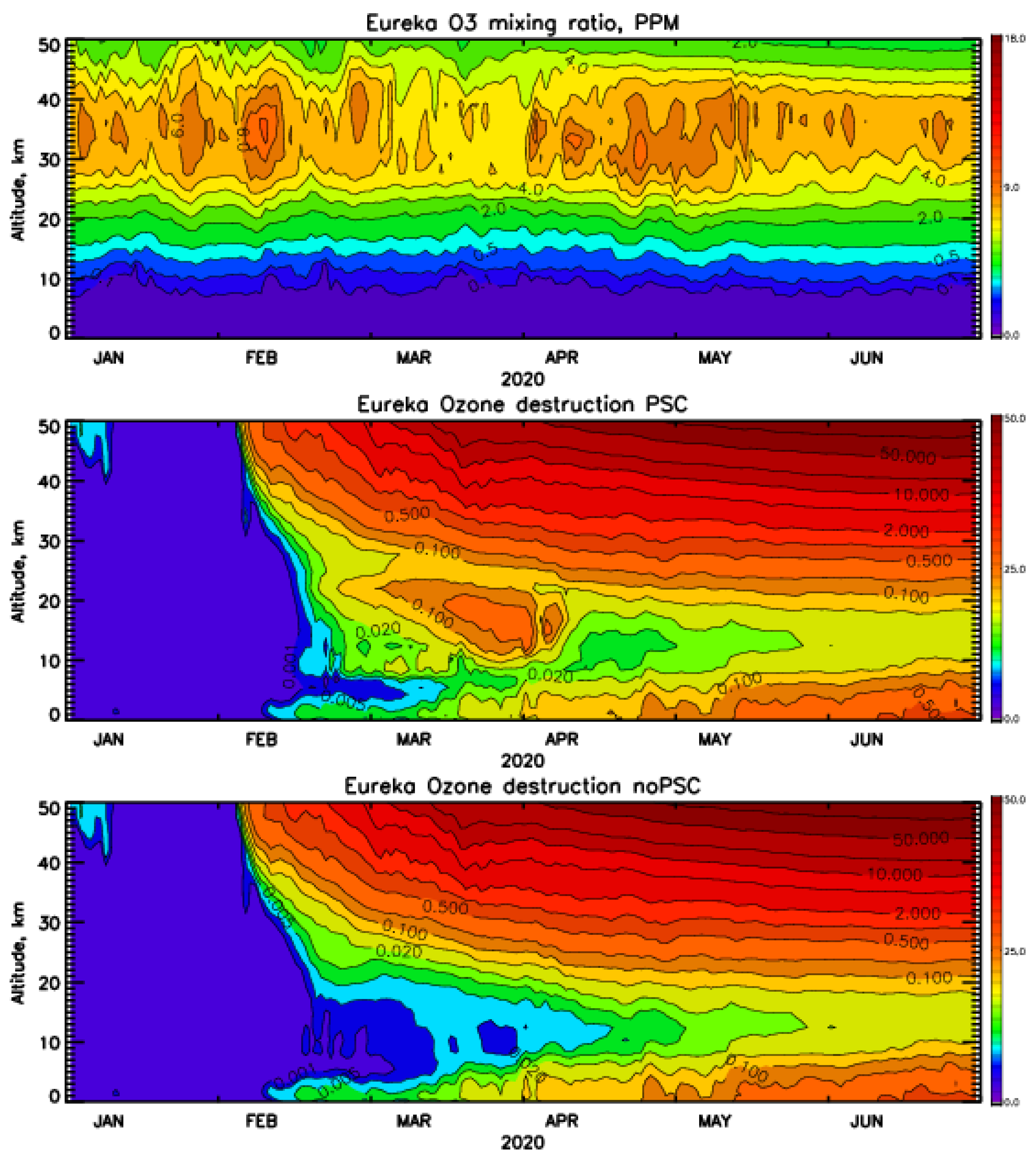
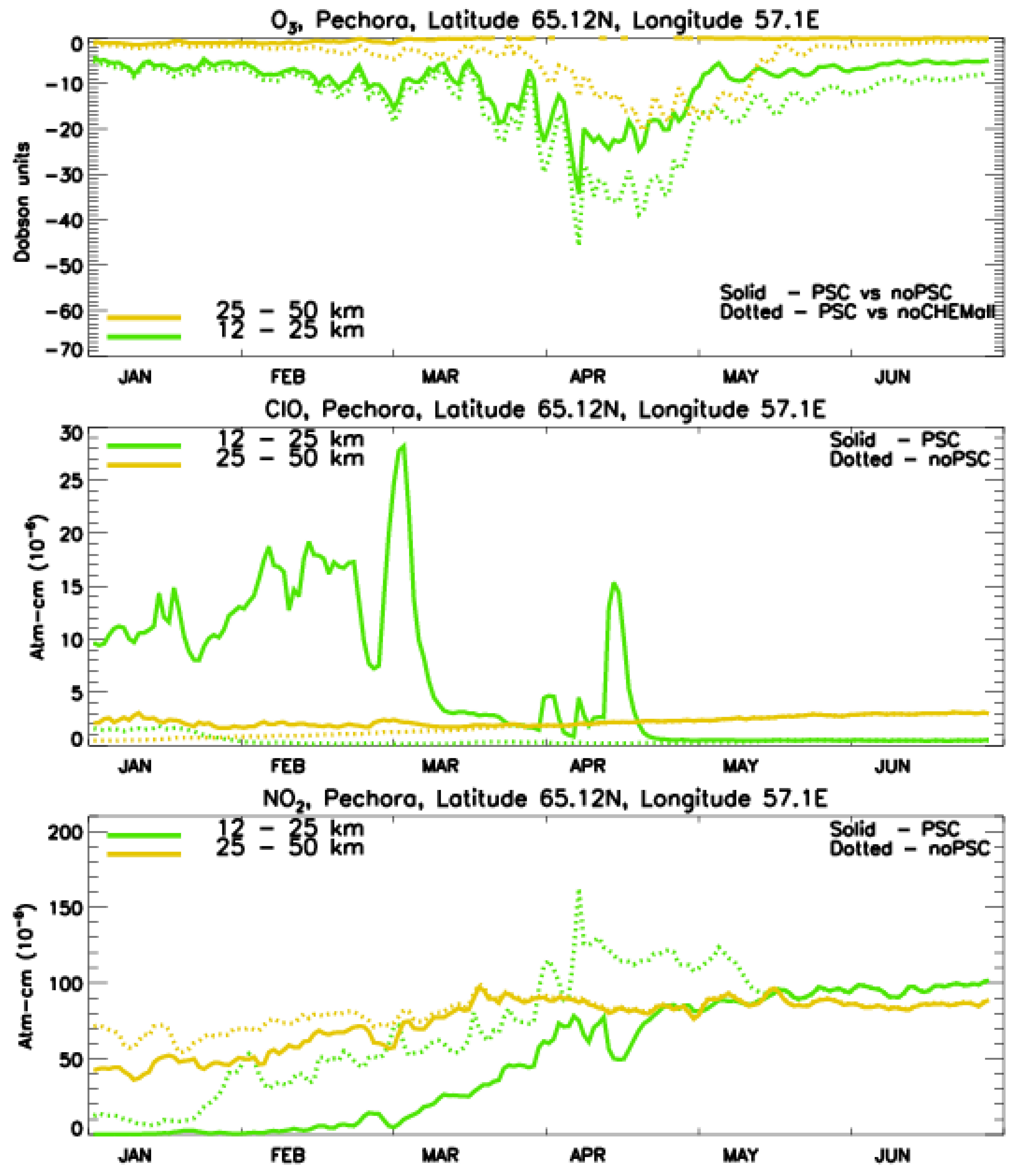
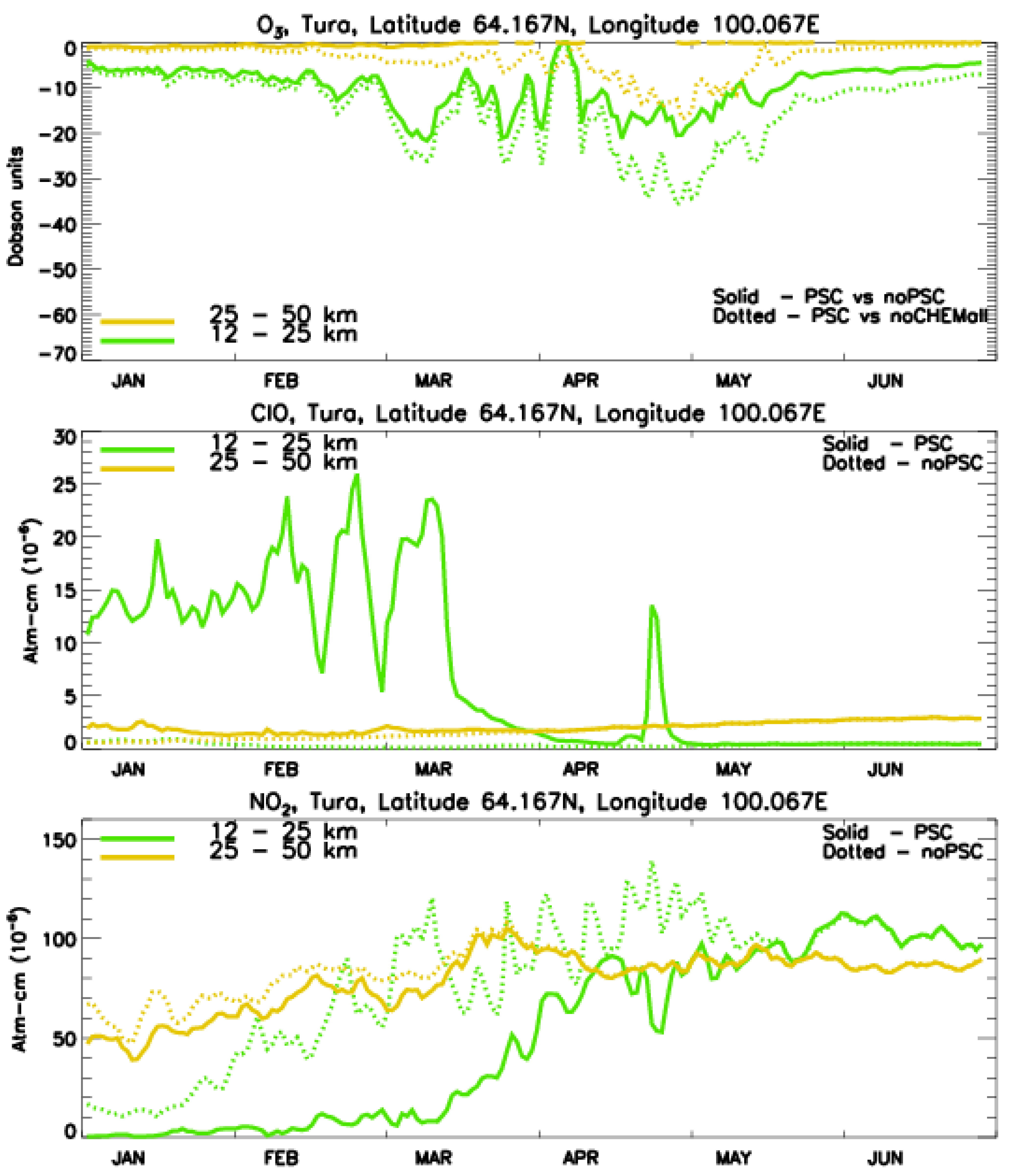
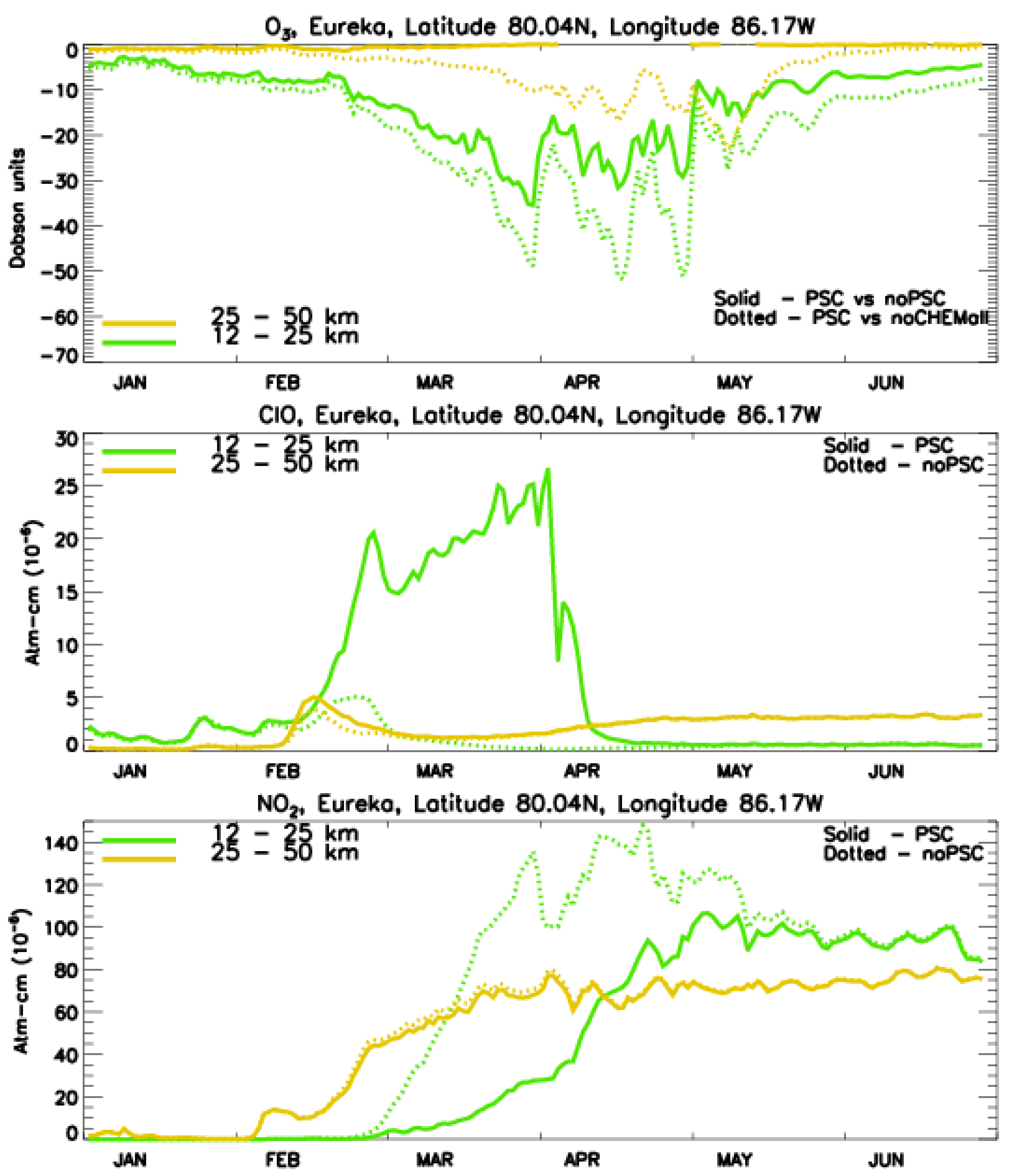
3.2. Ozone Loss over Selected Ozonometric Stations Using Chemistry-Transport Modeling

The global chemistry transport model of the lower and middle atmosphere was used to study the effect of chemical and Dynamic processes on the variability of the total column ozone (TCO) at selected ozonometric stations of the World Ozone and Ultraviolet Radiation Data Centre (WOUDC) network located in the Arctic. Two stations (Pechora and Tura) are located in the Eastern Hemisphere and two stations (Resolute and Eureka) are located in the Western Hemisphere. The results of the model calculations of the total ozone content over the period from 1 July 2019 to 30 June 2020 at the selected stations were compared with the satellite measurements of OMI, the average climatology of the SBUV for 1979–2019, and the MERRA-2 re-analysis data. SBUV data were selected because they cover a longer period than OMI data. Comparison of the data of model calculations and satellite observations of OMI with the average climatology of SBUV made it possible to assess the influence of the specific Dynamic conditions of winter 2019–2020 on the column ozone variability at the selected stations. To assess the influence of Dynamic and chemical factors on the TCO variability, in addition to the basic model experiment (PSC), additional model experiments were carried out, in which all chemistry was switched off from 1 December 2019 to 15 May 2020 at altitudes below 10 mb (noCHEM experiment) and the formation of PSCs was turned off (experiment noPSC).

Figure 7, Figure 8, Figure 9 and Figure 10 show the results of calculations of changes in the TCO, as well as the deviation of the noCHEM scenario from the average climatology of the SBUV and the baseline scenario from additional scenarios with one or another shutdown of chemistry in the lower stratosphere in the winter–spring period (bottom). Comparison of the results of CTM calculations with the OMI data measurements and MERRA-2 reanalysis demonstrated that the CTM with a rather coarse spatial resolution reproduced well the morphology of the TCO change recorded by OMI satellite measurements. At the same time, for the most abrupt TCO changes with the most often coinciding morphology of model calculations and satellite measurements, the amplitudes of quantitative TCO changes in model calculations were significantly less than in satellite observations. This was most likely the result of a rather coarse spatial resolution of the CTM used, although comparison with the data of the MEPRA-2 reanalysis, using a finer resolution, revealed that the MEPRA-2 results in the minima and maxima of the short-term TOC change also differed from the OMI results. In general, the difference between CTM and MERRA-2 was less than the difference between CTM and OMI and MERRA-2 and OMI observations. On the other hand, the difference between the CTM simulations and the MERRA-2/OMI during the period of maximum chemical destruction of ozone in March–April was less than in January–February, when the ozone variability was mainly determined by Dynamic processes.

At Pechora station (65.12° N, 57.1° E), located in the north of the European territory of Russia (Figure 7), one can note the formation of several local minima of the total ozone content with a characteristic time of several days in late January and mid and late February, which were reproduced qualitatively by model simulations for all three scenarios, which indicated the predominant role of Dynamic processes in the variability of the ozone content in winter. With the beginning of spring, the influence of chemical factors increases, which maximally affect the ozone depletion in April. In March, when the stratospheric polar vortex was located, for the most part, in the Western Hemisphere, at Pechora station, the ozone concentration values corresponded to the seasonal maximum, reaching values up to 450 DU.

By the end of March, when the polar vortex returns to the Eastern Hemisphere, total ozone content at Pechora drops by almost 50 percent, reaching values about 250 DU. Calculations according to the noCHEM scenario depicted that, as a result of the influence of Dynamic factors without taking into account any chemical destruction of ozone, its decrease from mid-March to mid-April reached 150 DU, and up to 90 DU compared to SBUV data. In this case, the chemical destruction of ozone, based on a comparison of the baseline and additional scenarios, amounted to 50 DU. Comparison of the difference in calculations according to the scenarios of PSC, noPSC, and noCHEM demonstrated that, in March–early April, most of the chemical destruction of ozone (the difference between PSC and noCHEM) was determined by heterogeneous processes with the participation of PSC (the difference between PSC and noPSC), whereas, in the middle of April, slightly less than half of the chemical destruction of ozone and the rest may be associated with a change in the gas-phase chemical destruction of ozone.

At another station, Tura (64.167° N, 100° E), located eastward to Pechora station, near the region of minimum values of the total ozone content in early spring, the minimum values were reached in the first half of March and the second half of April (Figure 8). During this time, the stratospheric polar vortex rotated around the pole, due to which the fluctuations in the total ozone content ranged from 250 DU in early March to 450 DU in the second half of March and again to 250 DU at the end of April. Analysis of the noCHEM scenario revealed that fluctuations in the total ozone content due to Dynamic factors amounted to more than 150 DU, and analysis of the model simulation results for different scenarios of switching off the chemical destruction of ozone demonstrated that the chemical destruction of ozone at Tura station was from 30 to 50 DU, of which about half (about 25 DU) was the destruction of ozone as a result of halogen activation on the surface of polar stratospheric clouds. At the same time, results of the noCHEM scenario comparison with the average SBUV data showed that, due to Dynamic factors, the decrease in the ozone content at Tura station was, on average, greater than at the Pechora station and exceeded 100 DU for some periods. Meanwhile, the difference between noPSC and noCHEM scenarios (green line), which characterized the role of gas-phase chemistry, depicted that, with a low significance of gas-phase destruction of ozone until mid-April, its role began to increase and reached 30 DU by the end of April–beginning of May. The role of destruction initiated by heterogeneous processes on the surface of the PSC, which prevails in March, became greater in April, but less than that of gas-phase destruction. It should be kept in mind that heterogeneous destruction can be greater than the gas-phase destruction but reduces the gas-phase destruction due to the interaction of nitrogen and halogen gases.

In the western part of the Arctic, at stations Resolute (74.72° N, 94.98° W) (Figure 9) and Eureka (80.04° N, 86.17° W) (Figure 10), the minimum values of the total ozone concentration (less than 250 DU) were observed in March: mid-March at Resolute station (Figure 9) and in the second part of March at Eureka station (Figure 10). Comparison of the calculation results for different scenarios indicated that the influence of Dynamic factors in the Western Hemisphere was more significant than in the Eastern Hemisphere, since, for the noCHEM scenario comparison to SBUV climatic data, the total content fluctuated in the order of 100–150 DU. As can be seen from the comparison of the baseline scenario with additional ones, the chemical destruction of ozone also ranged from 50 to 60 DU, which was slightly higher than in the Eastern Hemisphere. At the same time, in April, chemical factors for ozone destruction prevailed over Dynamic factors at western stations. It should also be noted that there were two peaks of maximum chemical destruction of ozone: in late March and mid-April. At the same time, chemical destruction in the second half of March was superimposed on a Dynamic decrease in its content, which led to a minimum in the seasonal variation of the total ozone content, while in April, when the chemical destruction of ozone was even greater than in March, the polar vortex was already shifting towards the eastern hemisphere (Figure 1), and the total ozone content was higher than in March.

Comparison of the CTM simulation results for different scenarios for Resolute station demonstrated (Figure 9) that heterogeneous destruction prevailed over gas-phase destruction during March, and in April their role was approximately the same. It should be kept in mind that the polar vortex was stable in the Western Hemisphere for most of March, and in April it only covered some areas of the Western Hemisphere. Because of this, the ozone content above Resolute in April differed significantly less from the average climatic values than in March. Therefore, the detected almost identical two maxima of chemical destruction of ozone at the end of March and the end of April (bottom of Figure 9) were superimposed on different values of the total column ozone, which in April was significantly higher than in March. In addition, it should be kept in mind that the role of heterogeneous destruction is fact that, with an increase in significantly underestimated due to the halogen gas radicals after heterogeneous activation on the surface of PSC, the concentration of nitrogen radicals and, consequently, the role of nitrogen catalytic cycles can decrease. The same situation was registered for Eureka station.

For three periods of maximum ozone decrease as a result of chemical processes (red line at the bottom of Figure 10) exceeding 50 DU, in March most of it can be attributed to heterogeneous ozone destruction, and in April the role of heterogeneous and gas-phase destruction is similar. At the same time, it should be stated again that the actual role of heterogeneous ozone destruction may be greater due to the fact that the role of gas-phase ozone destruction in nitrogen catalytic cycles may decrease when nitrogen radicals bind with chlorine and bromine gases after their sharp increase after heterogeneous activation. The deviation of the ozone content in the column in March at the Eureka station from the climatic ones reached 150 DU and more, which indicated the predominant role of the Dynamic processes of ozone reduction, exceeding chemical destruction by three times.

Figure 11 presents the annual variation of the vertical distribution of the ozone-mixing ratio (top), as well as the coefficient of chemical destruction of odd oxygen, for the scenarios PSC (middle) and noPSC (bottom), calculated using CTM. Increased destruction of odd oxygen, the content of which in the lower stratosphere is almost completely determined by ozone, is observed from early February to mid-April at altitudes from 15 to 25 km. In this case, several local maxima of the destruction of odd ozone were noted, the most significant of which were the maxima in late February–early March and in mid-April, which corresponded to a local decrease in the ratio of the ozone-mixing ratio.

For the scenario without taking into account the formation of PSCs (noPSC) in the area of the Pechora station, there was no local increase in the rate of destruction of odd oxygen, although an increase in the gas-phase destruction of odd oxygen was noted during the spring, both at the heights of the lower and upper stratospheres. No localized increase in the rate of gas-phase destruction of odd oxygen in the region of decrease in the ratio of the ozone-mixing ratio was observed in the noPSC scenario, as could be expected based on the obtained difference in the total ozone content for noCHEM and noPSC scenarios, which is especially significant in April (Figure 7).

Tura station, as well as Pechora located in the Eastern Hemisphere, was also characterized by a localized increase in the rate of destruction of odd oxygen in February, March, and April for the PSC scenario and the absence of zones of a local increase in the gas-phase increase in the decomposition of odd oxygen in the noPSC scenario (Figure 12). The difference between the Pechora and Tura stations lies in the later formation of zones of increased destruction of odd oxygen for the PSC scenario over the Tura than over the Pechora, both in February and in March and April.

Figure 13 and Figure 14 present the variability of the ozone-mixing ratio, as well as the rate of destruction of odd oxygen for the stations of the Western Hemisphere Resolute and Eureka. These stations were characterized by the formation of one large zone of an increase in the rate of destruction of odd oxygen for the PSC scenario at altitudes of 12–25 km throughout March, in contrast to the stations of the Eastern Hemisphere, for which the formation of several small zones of an increase in the rate of destruction of odd oxygen was noted (Figure 11 and Figure 12). Accordingly, in the Western Hemisphere in March, the most significant decrease in both the ratio of the ozone mixture and its total content was recorded (Figure 9 and Figure 10). At the same time, a significant decrease in the ozone-mixing ratio was noted not only in the lower but also in the upper stratosphere. For the noPSC scenario for stations in the Western Hemisphere, zones of increased rate of gas-phase destruction of odd oxygen were also not recorded. The difference between the stations Resolute and Eureka lies in the later return of the Sun after the polar night at the Eureka station, as a result of which the chemical destruction of ozone in the upper stratosphere becomes significant only from the second half of February. In addition, one can note the formation of a small additional zone of destruction of odd oxygen at the Eureka station, in contrast to the Resolute station.

Figure 15, Figure 16, Figure 17 and Figure 18 demonstrate the change in the ozone content, as well as ClO and NO2, which determine the rates of destruction of odd oxygen in chlorine and nitrogen catalytic cycles for the selected ozonometric stations separately for the lower (12–25 km) and upper (25–50 km) stratosphere. For the ozone content, the difference is given for the scenarios of PSC and noPSC (solid lines) and PSC and noCHEM (dots), and for ClO and NO2, the total content in layers is in atm-cm. At all stations, a common feature was the main decrease in the ozone content in the lower stratosphere, both for the difference between the PSC scenario and the noPSC scenario, and for the difference with the noCHEM scenario. In the upper stratosphere, the difference was noted only for the noCHEM scenario and, mainly, in April. Again, for all stations, an increase in the ClO content in the lower stratosphere was noted for the PSC scenario during periods of an increase in the rate of destruction of odd oxygen (Figure 11, Figure 12, Figure 13 and Figure 14), which indicated the dominant role of ozone destruction in halogen catalytic cycles after the heterogeneous activation of halogens on the surface of polar stratospheric clouds. Nitrogen dioxide, again for all stations, was characterized by an increased value of the content in the lower stratosphere for the noPSC scenario as compared to the PSC scenario. This suggests, on the one hand, that, despite the fact that denitrification in the Arctic was less pronounced than in the Antarctic, chemical reactions with the participation of chlorine and nitrogen gases as a result of heterogeneous activation on the surface of the PSCs led to a redistribution of gases of the NOx family towards reductions in nitrogen dioxide, which, on the other hand, had the potential to reduce ozone depletion in nitrogen catalytic cycles in the PSC scenario versus the noPSC scenario. Thus, a significant difference between the change in ozone in the scenarios noPSC and noCHEM arose not due to an increase in the rate of ozone destruction in nitrogen catalytic cycles, which was additional to the destruction in halogen cycles after heterogeneous activation on the PSCs, but as a result of a decrease in nitrogen destruction of ozone in the PSC scenario, compared to the noPSC scenario.

The differences between the stations in the distribution of the main gases affecting the chemical destruction of stratospheric ozone were mainly associated with the time of their stay in the polar vortex region, which can be seen from the increased content of ClO. At Pechora station, two large maxima were noted, in early March and the first half of April, and several small maxima in January–February and at the junction of March and April (Figure 15), while at Tura station there were several almost identical maxima in February–the first half March and one in the second half of April. These maxima also corresponded to the periods of the most significant chemical ozone reduction (top Figure 15 and Figure 16). At the same time, for Tura station in late March–early April, several minima of the ozone content in the PSC scenario were noted during periods of the absence of a local increase in ClO (Figure 16). The same periods were characterized by a short-term increase in the content of NO2, which was not associated with an increase in the content of ClO (bottom of Figure 16), but, judging from the top of Figure 16, was associated with heterogeneous processes on the surface of the PSC. Thus, the decrease in the ozone content in these situations can be determined by the increase in destruction in nitrogen cycles. In addition, heterogeneous processes, when the station is not inside the vortex, but is located near it, can also lead to a local decrease in ozone.

For the stations of the Western Hemisphere (Figure 17 and Figure 18), it was characteristic that an increased content of ClO was retained for the PSC scenario during February–March. At the same time, the decrease in the ozone content in the PSC scenario with respect to the noPSC scenario in the lower stratosphere increased more or less uniformly during this period, reaching a maximum in late March–early April. Earlier ClO maxima, as, for example, at the beginning of February at the Resolute station (Figure 17), did not lead to a significant increase in the rate of destruction of odd oxygen (Figure 13), probably due to insufficient concentrations of atomic oxygen in the conditions of low insolation.

In April, at both stations, in the absence of an increased ClO content, a decrease in the ozone content of the lower stratosphere was registered in the PSC scenario as compared to the noPSC scenario. At the same time, there was also a decrease in the content of NO₂ in the PSC scenario as compared to the noPSC scenario. Thus, in April, in contrast to March, the local chemical destruction of ozone in the lower stratosphere of the stations of the Western Hemisphere in both chlorine and nitrogen cycles was insignificant, as can be seen from the estimates of the total destruction of odd oxygen (Figure 13 and Figure 14). Nevertheless, in April, at stations in the Western Hemisphere, episodes of a significant decrease in ozone content were also noted (Figure 9 and Figure 10), largely associated with the processes of PSC formation (Figure 17 and Figure 18). As can be seen from the figures of the potential vorticity distribution at 475 K and the temperature of the lower stratosphere, in April the polar vortex was mainly located in the Eastern Hemisphere, while the Resolute and Eureka stations were, at that time, near the edge of the polar vortex. Thus, it can be assumed that heterogeneous processes with the participation of PSC influenced the ozone content not only inside the vortex, but also its content near the edge outside the polar vortex.

4. Discussion

The 2019–2020 winter was characterized by an unusually stable and cold stratospheric polar vortex in the Arctic with low temperatures close to the record values of the winter seasons of 1996–1997 and 2010–2011 over the past 60 years. The reason for such low temperature of the Arctic stratosphere was the weakened propagation of wave activity from the troposphere, especially in February–early March 2020 and the downward reflection of wave activity in the upper stratosphere.

The minor SSW event in late March 2020 led to an increase in the Arctic stratosphere temperature that was strongest in the upper stratosphere. However, we assumed that the impact of this SSW event was not negligible for the polar lower stratosphere and it contributed to a decrease of PSC nitric acid trihydrate (NAT) volume, reduced from ~50 mln km³ (on 17–18 March) to nearly zero in the last days of March. Certainly, the seasonal cycle was the other important cause of PSC NAT volume decrease.

The enhancement of wave activity propagation over the Gulf of Alaska could be important but not a sole factor responsible for the onset of the SSW event in late March 2020 as it is supposed that only 30%/60% of SSW events are preceded by extreme wave activity episodes at the lower troposphere/lower stratosphere (White et al., 2019). Therefore, numerical experiments are desirable to verify a role of this enhanced wave activity propagation in the onset of this minor SSW event. The weakened propagation of wave activity from the troposphere to the stratosphere could be caused, in addition to other factors, by the positive temperature anomalies in the troposphere over northeastern Eurasia. However, the weakening of wave activity propagation to the stratosphere could be not only due to changes in the troposphere but in the stratosphere, too. Therefore, our speculation needs further research.

During the 2020 spring, when the photochemical processes of ozone destruction intensified after the polar night, the polar vortex in March was mainly in the Western Hemisphere, and in April, in the Eastern Hemisphere. This created a basis for comparing the influence of Dynamic and chemical processes on the variability of stratospheric ozone in the Western and Eastern Hemispheres, because in March, gas-phase photochemical processes were less active than in April. Therefore, two stations located in the Eastern Hemisphere and two stations located in the Western Hemisphere were selected for analysis.

The results of the numerical experiments with the chemical transport model demonstrated that both heterogeneous and gas-phase chemical processes played an important role in the destruction of polar ozone in the spring. Comparison of the results of the model experiments with switched-off processes of formation and evolution of PSCs (scenario noPSC) with the results of calculations in which ozone was considered as an inert tracer in the lower stratosphere (scenario noCHEM) showed that gas-phase ozone destruction played an insignificant role in March (the difference between scenarios was less than 10 DU), and it grew significantly in April (up to 30 DU). At the same time, in the Western Hemisphere, the gas-phase destruction of ozone already increased significantly at the end of March, while in the Eastern Hemisphere it remained low throughout March. When the processes of formation and evolution of polar stratospheric clouds were connected (PSC scenario), on the one hand, heterogeneous activation of halogen gases on their surface was activated, which led to a sharp increase in chlorine and bromine destruction of ozone. However, on the other hand, the role of gas-phase ozone destruction in nitrogen catalytic cycles decreased due to denitrification, which in the Arctic was less significant than in the Antarctic. However, under conditions of low stratospheric temperatures during the 2020 winter and spring, it played a certain role in the redistribution of nitrogen gases as a result of their interaction with increased halogen radicals.

Consideration of the difference in model simulations for scenarios PSC and noPSC, and noPSC and noCHEM showed that, in the total balance of ozone depletion in March, the addition of heterogeneous destruction prevailed over the reduction in gas-phase ozone destruction, as a result of which the difference between PSC and noPSC was greater than the difference between noPSC and noCHEM. This was typical for both hemispheres, although in the Western Hemisphere, where the polar vortex was located for most of March, the difference was greater. In April, when photochemical processes intensify and there are fewer polar stratospheric clouds, the decrease in destruction in nitrogen catalytic cycles became greater than the increase in destruction in halogen cycles of ozone destruction in the eastern hemisphere, where the vortex was present for most of the month; in the western hemisphere, these two factors were close to being equal. As a result, for stations in the Eastern Hemisphere, the difference between the PSC and noPSC scenarios became smaller than that between the noPSC and noCHEM scenarios, and the addition of heterogeneous chemistry practically did not change the degree of ozone depletion in the Western Hemisphere.

5. Conclusions

In general, a comparison of the influence of Dynamic and photochemical factors on the variability of the Arctic stratospheric ozone in the spring of 2020 showed that, based on the analysis of the difference between the noCHEM scenario and SBUV climatology, it was concluded that the specific Dynamic conditions of winter–spring 2019–2020 described a decrease in ozone up to 100 DU in the Eastern Hemisphere and over 150 DU in the Western Hemisphere. In this case, the photochemical destruction of ozone in both the Western and Eastern hemispheres at a maximum was about 50 DU with peaks in April in the Eastern Hemisphere and in March and April in the Western Hemisphere. In this case, the maximum photochemical ozone destruction was superimposed on the influence of Dynamic factors during the period when the polar vortex was in the Eastern Hemisphere in early March and mid-April and in the Western Hemisphere in mid and late March, when the maximum ozone reduction was registered.

Overall, the main conclusions of our study are as follows:

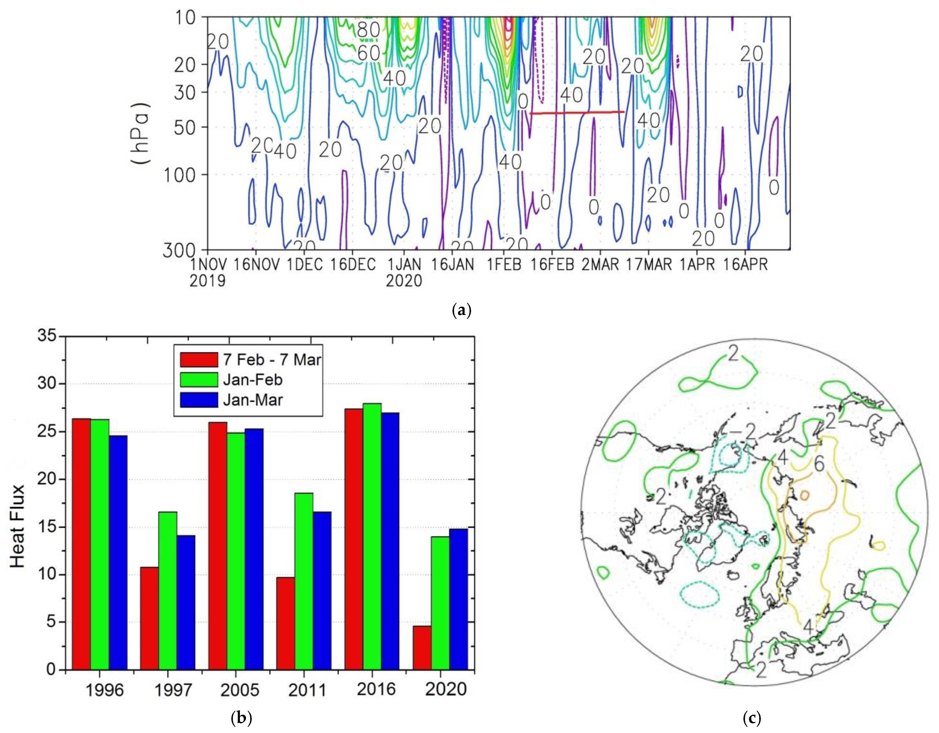
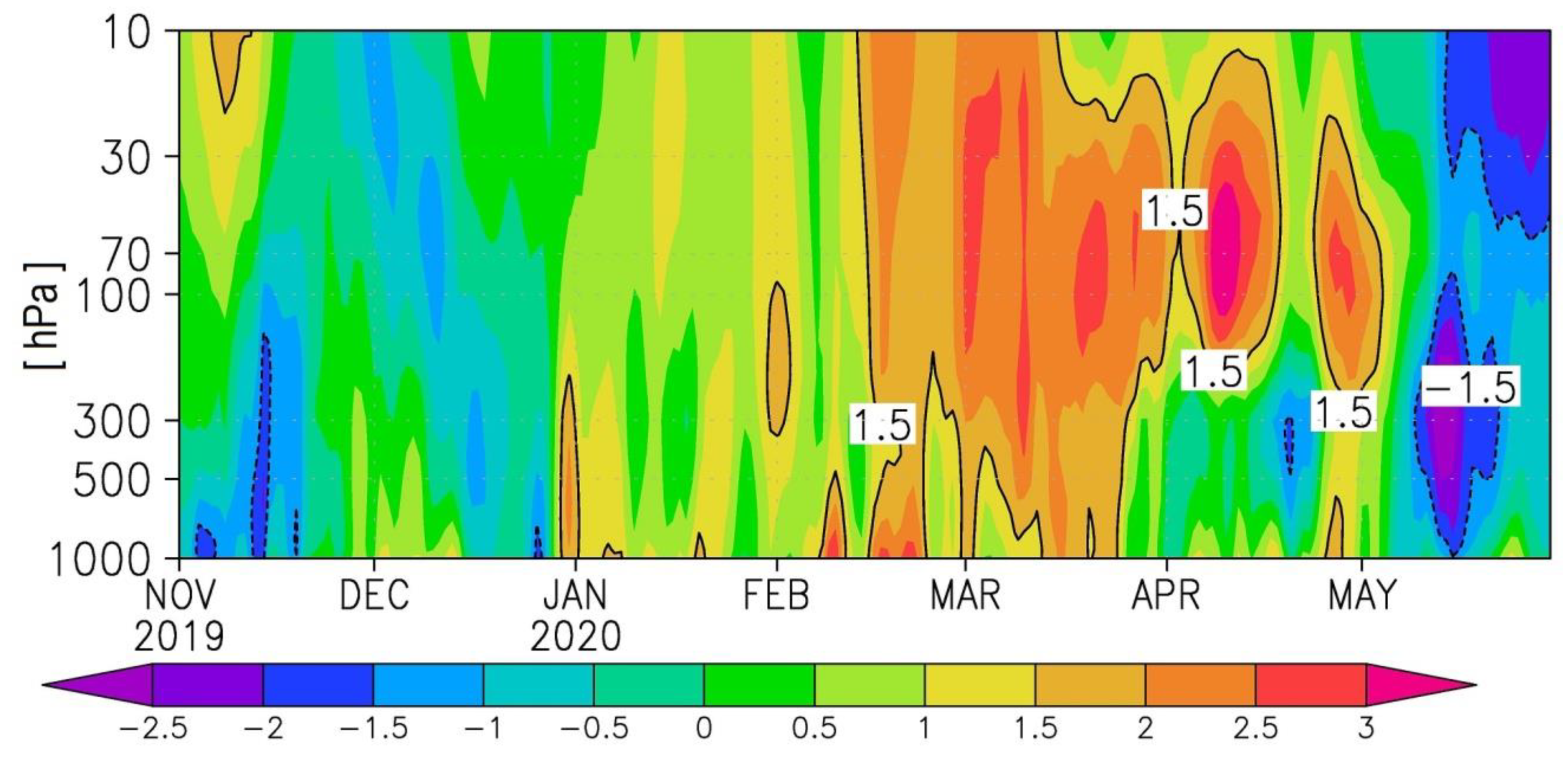
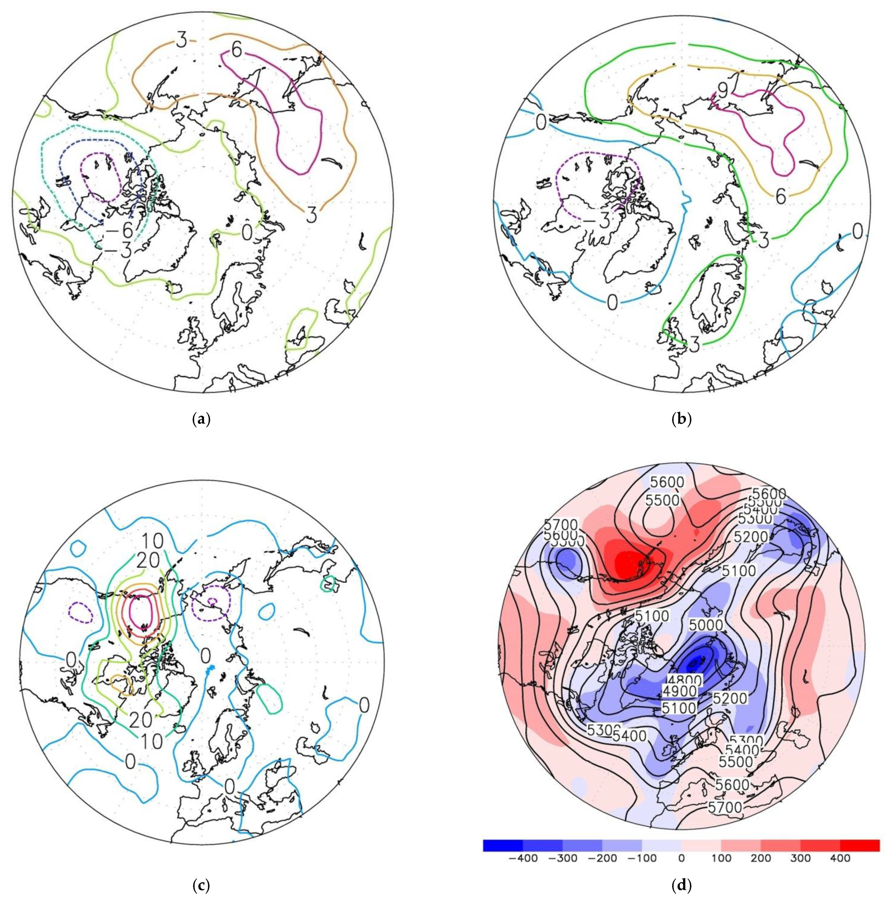
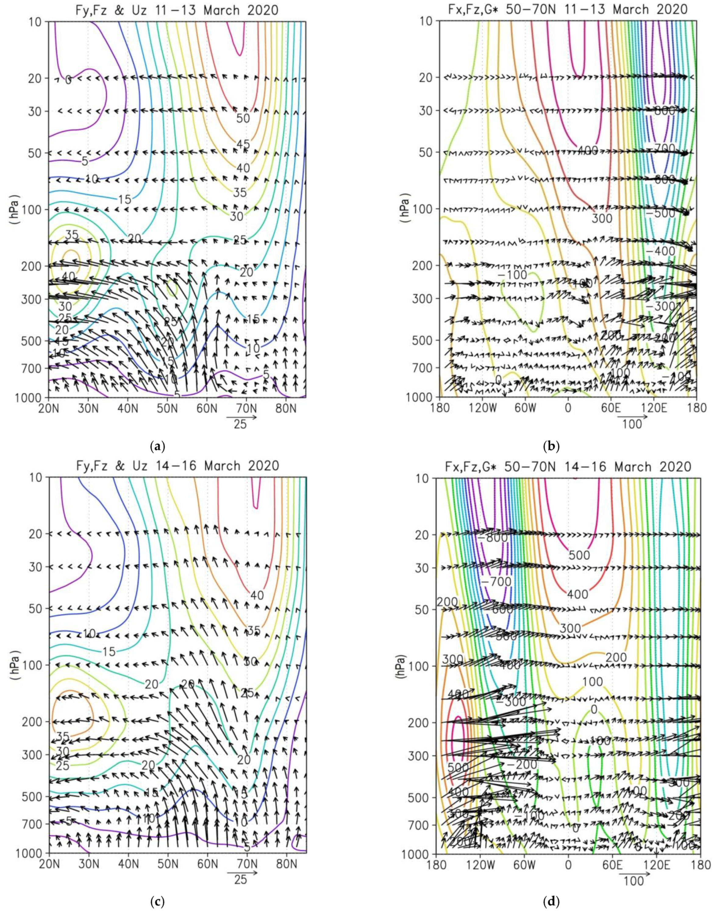
• The enhancement of wave activity propagation over the Gulf of Alaska in the middle of March contributed to the onset of the minor SSW event and to an increase in the Arctic stratosphere temperature.
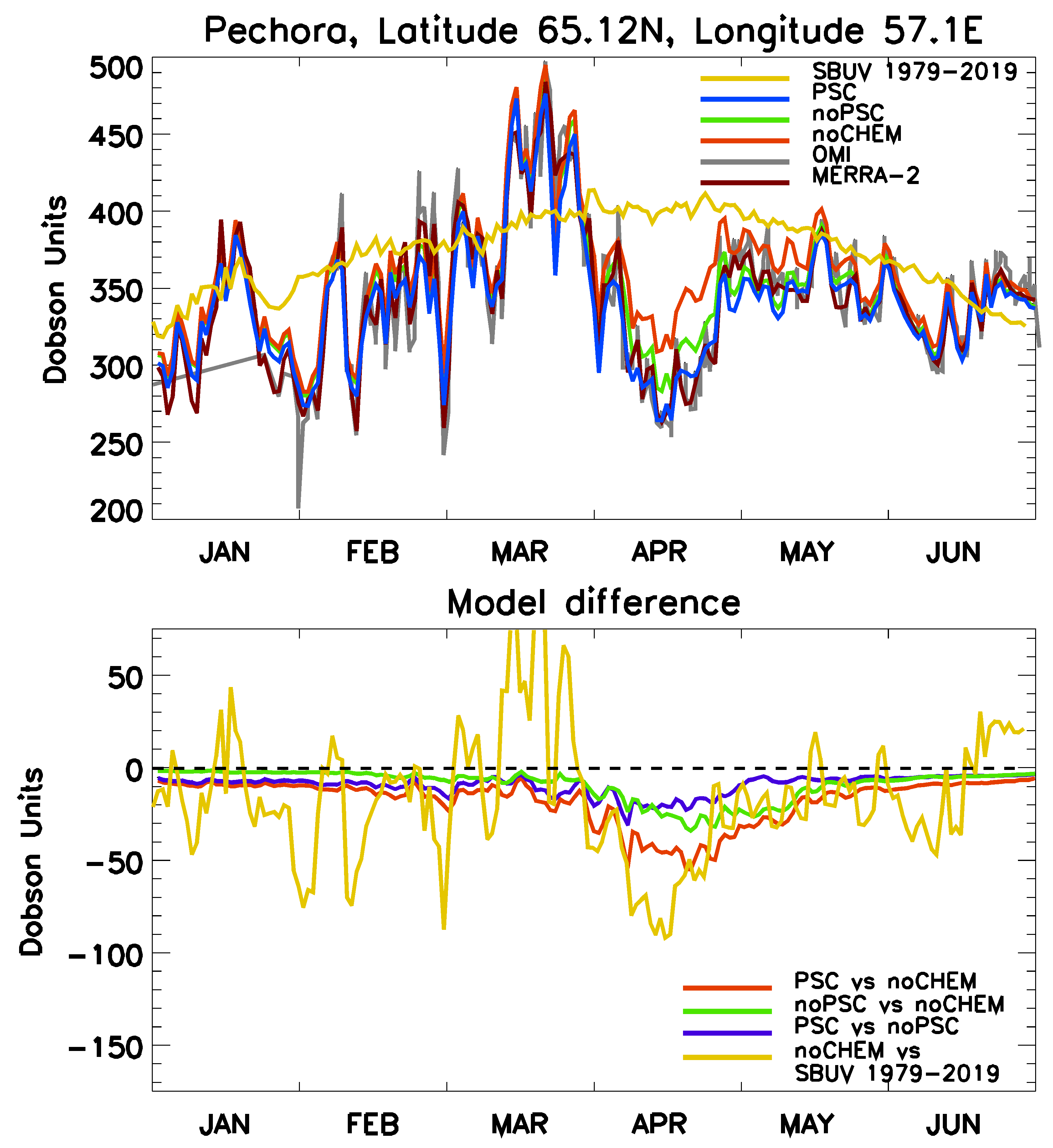
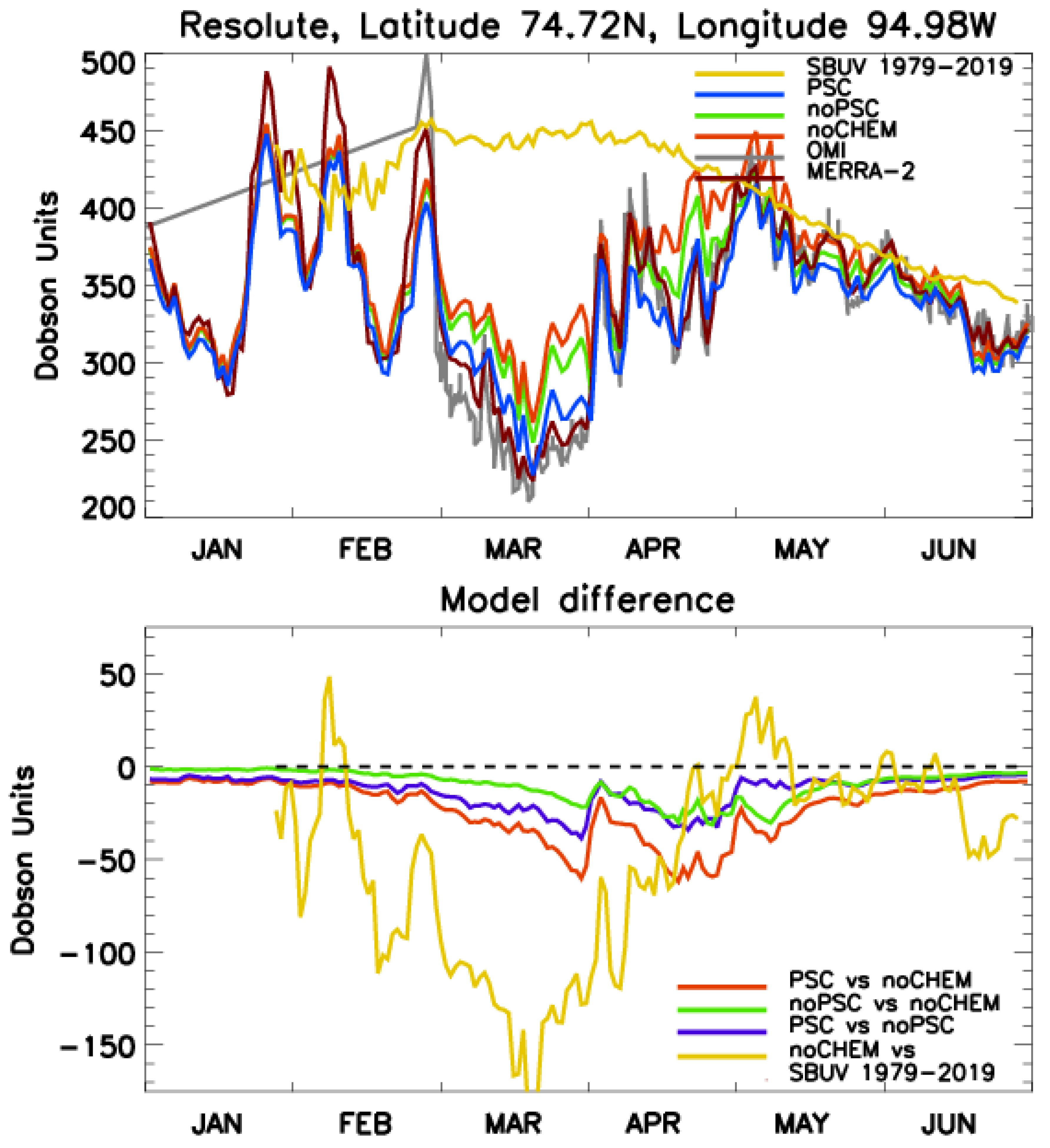
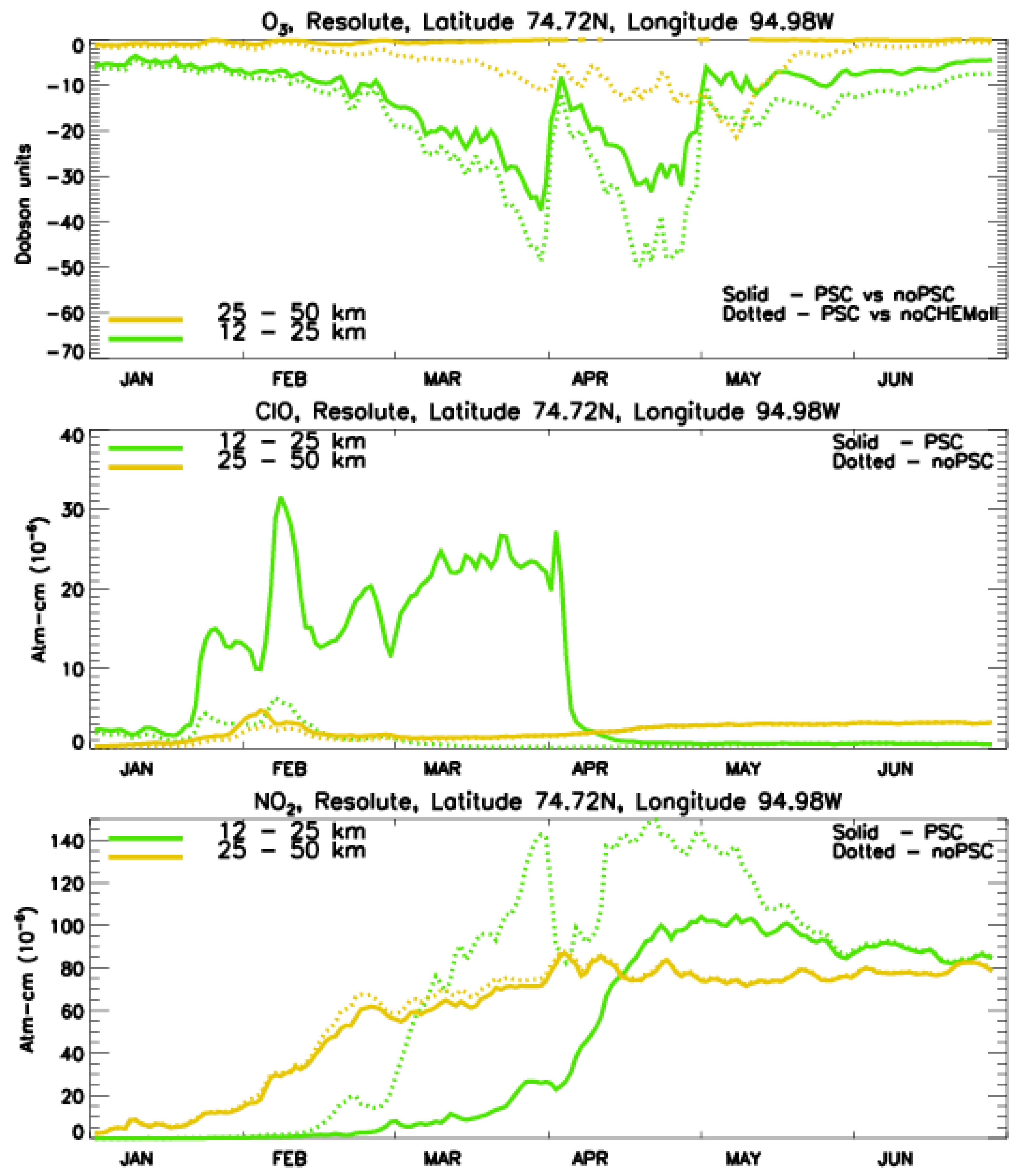
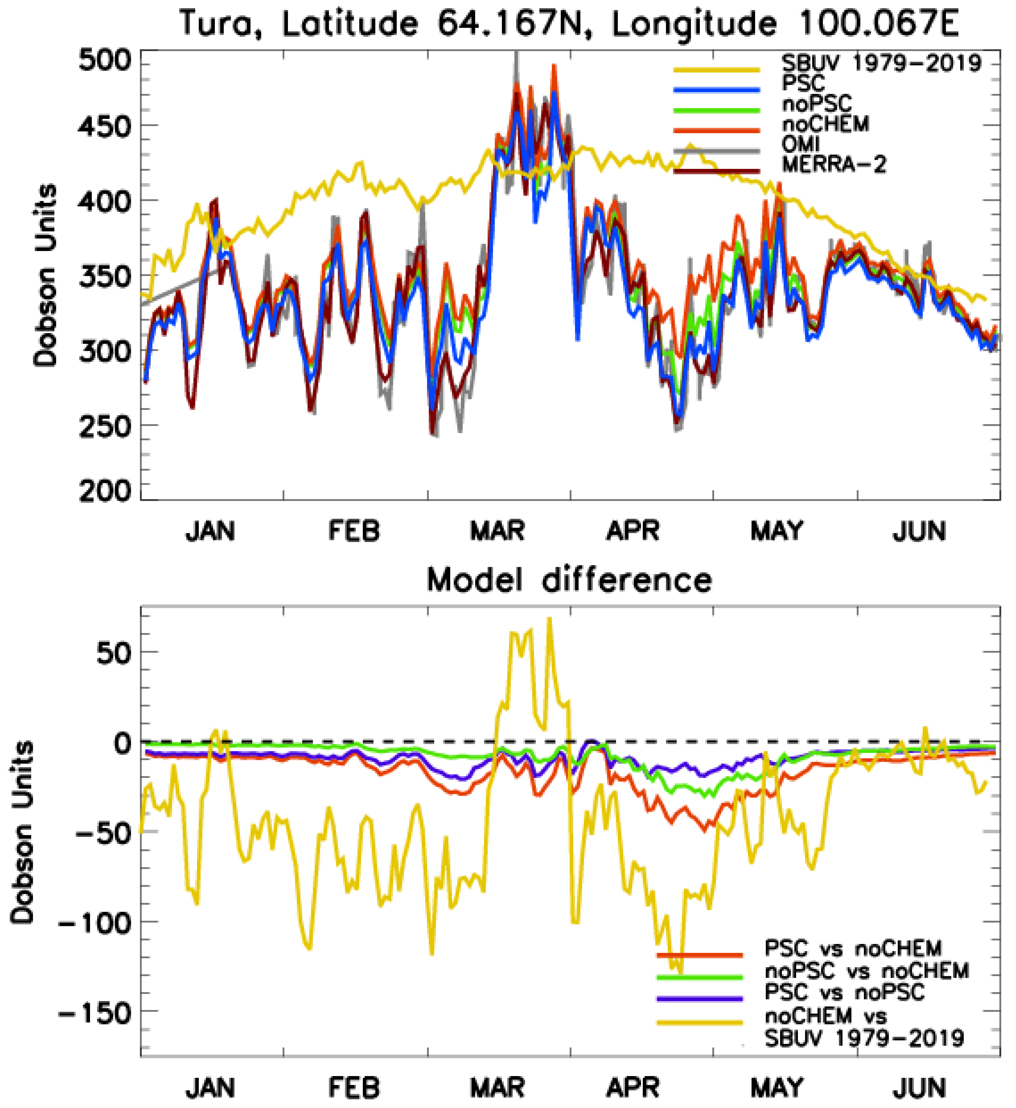
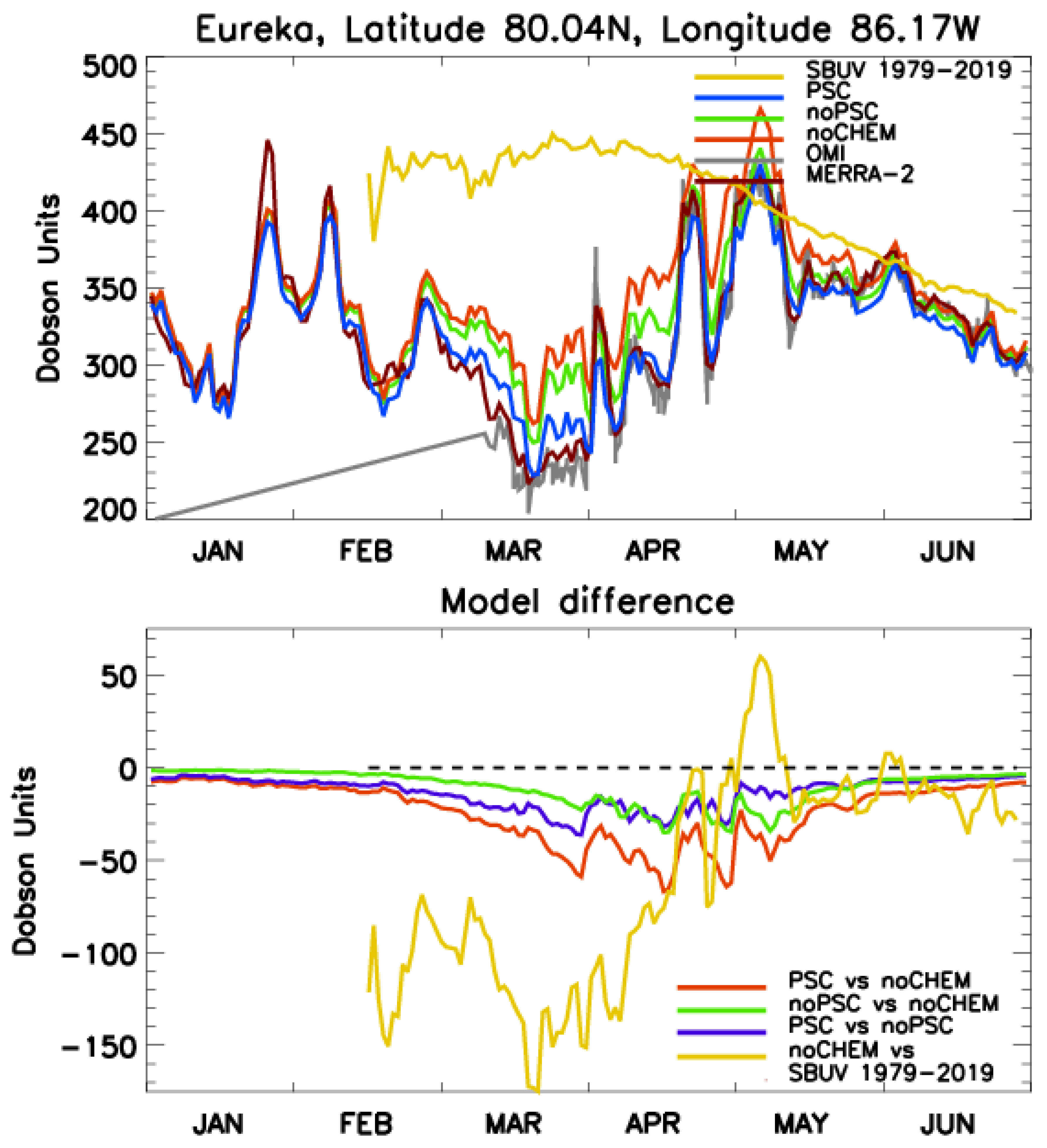
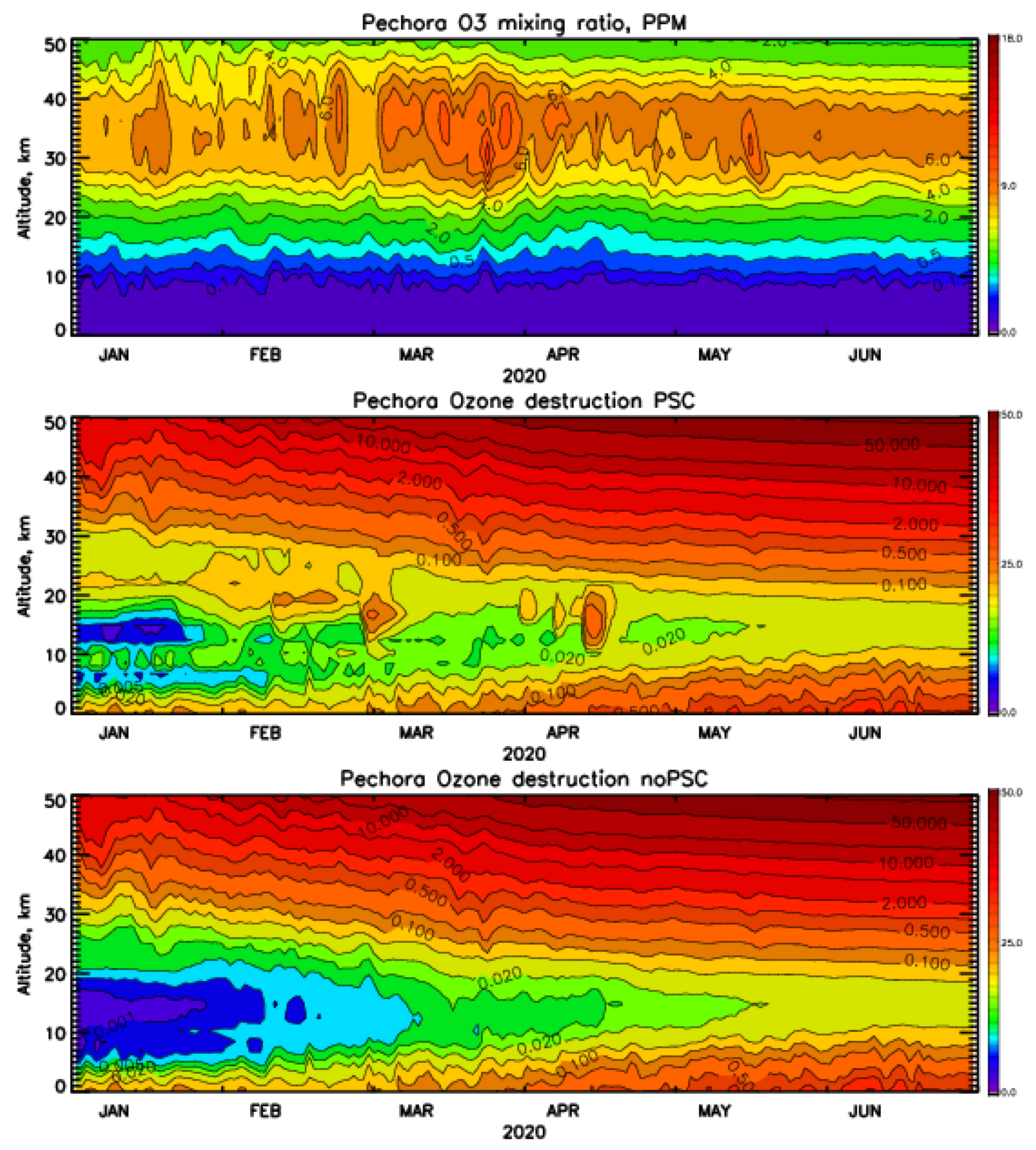
• The results of numerical calculations using CTM with Dynamic parameters specified from the MERRA-2 reanalysis data, carried out according to several scenarios of accounting for the chemical destruction of ozone, demonstrated that both Dynamic and chemical processes make a significant contribution to ozone changes over ozonometric stations, both in the Eastern and in the Western Hemispheres. Heterogeneous activation of halogen gases on the surface of polar stratospheric clouds, on the one hand, leads to a sharp increase in the destruction of ozone in chlorine and bromine catalytic cycles, and, on the other hand, decreases its destruction in nitrogen catalytic cycles.

It should be noted that the results presented in this article were obtained using only one chemistry-transport model with a rather coarse spatial resolution. In addition, the Dynamic parameters were set only from MERRA-2 reanalysis data. This imposes certain limitations on the conclusions obtained in this article and requires further verification using models with higher resolution and other reanalysis data. In addition, the conclusions of this article for winter 2019–2020 would be interesting to compare with other winters, when Arctic ozone loss was registered.

References

1. Tegtmeier, S.; Rex, M.; Wohltmann, I.; Kruger, K. Relative importance of dynamical and chemical contributions to Arctic wintertime ozone. Geophys. Res. Lett. 2008, 35, L17801. [Google Scholar] [CrossRef] [Green Version]
2. Kidston, J.; Scaife, A.A.; Hardiman, S.C.; Mitchell, D.; Butchart, N.; Baldwin, M.P.; Gray, L. Stratospheric influence on tropospheric jet streams, storm tracks and surface weather. Nat. Geosci. 2015, 8, 433–440. [Google Scholar] [CrossRef]
3. Nath, D.; Chen, W.; Zelin, C.; Pogoreltsev, A.I.; Wei, K. Dynamics of 2013 Sudden Stratospheric Warming event and its impact on cold weather over Eurasia: Role of planetary wave reflection. Sci. Rep. 2016, 6, 24174. [Google Scholar] [CrossRef]
4. Peters, D.H.; Schneidereit, A.; Karpechko, A.Y. Enhanced Stratosphere/Troposphere Coupling During Extreme Warm Stratospheric Events with Strong Polar-Night Jet Oscillation. Atmosphere 2018, 9, 467. [Google Scholar] [CrossRef] [Green Version]
5. King, A.D.; Butler, A.H.; Jucker, M.; Earl, N.O.; Rudeva, I. Observed Relationships Between Sudden Stratospheric Warmings and European Climate Extremes. J. Geophys. Res. Atmos. 2019, 124, 13943–13961. [Google Scholar] [CrossRef]
6. Matthias, V.; Kretschmer, M. The Influence of Stratospheric Wave Reflection on North American Cold Spells. Mon. Weather. Rev. 2020, 148, 1675–1690. [Google Scholar] [CrossRef]
7. Funke, B.; Ball, W.; Bender, S.; Gardini, A.; Harvey, V.L.; Lambert, A.; López-Puertas, M.; Marsh, D.R.; Meraner, K.; Nieder, H.; et al. HEPPA-II model–measurement intercomparison project: EPP indirect effects during the dynamically perturbed NH winter 2008–2009. Atmospheric Chem. Phys. Discuss. 2017, 17, 3573–3604. [Google Scholar] [CrossRef] [Green Version]
8. Zülicke, C.; Becker, E.; Matthias, V.; Peters, D.H.W.; Schmidt, H.; Liu, H.-L.; Ramos, L.D.L.T.; Mitchell, D.M. Coupling of Stratospheric Warmings with Mesospheric Coolings in Observations and Simulations. J. Clim. 2018, 31, 1107–1133. [Google Scholar] [CrossRef]
9. Smyshlyaev, S.P.; Pogoreltsev, A.I.; Galin, V.Y.; Drobashevskaya, E.A. Influence of wave activity on the composition of the polar stratosphere. Geomagn. Aeron. 2016, 56, 95–109. [Google Scholar] [CrossRef]
10. World Meteorological Organization (WMO). Scientific Assessment of Ozone Depletion: 2018; Global Ozone Research and Monitoring Project—Report No. 58; Meteorological Organization: Geneva, Switzerland, 2018; p. 588. [Google Scholar]
11. Solomon, S.; Haskins, J.; Ivy, D.J.; Min, F. Fundamental differences between Arctic and Antarctic ozone depletion. Proc. Natl. Acad. Sci. USA 2014, 111, 6220–6225. [Google Scholar] [CrossRef] [PubMed] [Green Version]
12. Rex, M.; Harris, N.R.P.; von der Gathen, P.; Lehmann, R.; Braathen, G.O.; Reimer, E.; Beck, A.; Chipperfield, M.; Alfier, R.; Allaart, M.; et al. Prolonged stratospheric ozone loss in the 1995–96 Arctic winter. Nat. Cell Biol. 1997, 389, 835–838. [Google Scholar] [CrossRef]
13. Lefèvre, F.; Figarol, F.; Carslaw, K.S.; Peter, T. The 1997 Arctic Ozone depletion quantified from three-dimensional model simulations. Geophys. Res. Lett. 1998, 25, 2425–2428. [Google Scholar] [CrossRef]
14. Rex, M.; Salawitch, R.J.; Harris, N.R.P.; von der Gathen, P.; Braathen, G.O.; Schulz, A.; Deckelmann, H.; Chipperfield, M.; Sinnhuber, B.-M.; Reimer, E.; et al. Chemical depletion of Arctic ozone in winter 1999/2000. J. Geophys. Res. Space Phys. 2002, 107, SOL-18. [Google Scholar] [CrossRef] [Green Version]
15. Manney, G.L.; Santee, M.L.; Froidevaux, L.; Hoppel, K.; Livesey, N.J.; Waters, J.W. EOS MLS observations of ozone loss in the 2004–2005 Arctic winter. Geophys. Res. Lett. 2006, 33. [Google Scholar] [CrossRef] [Green Version]
16. Manney, G.L.; Santee, M.L.; Rex, M.; Livesey, N.J.; Pitts, M.C.; Veefkind, P.; Nash, E.R.; Wohltmann, I.; Lehmann, R.; Froidevaux, L.; et al. Unprecedented Arctic ozone loss in 2011. Nat. Cell Biol. 2011, 478, 469–475. [Google Scholar] [CrossRef] [PubMed]
17. World Meteorological Organization (WMO). Scientific Assessment of Ozone Depletion: 2014; Global Ozone Research and Monitoring Project—Report No. 55; Meteorological Organization: Geneva, Switzerland, 2014; p. 416. [Google Scholar]
18. Manney, G.L.; Lawrence, Z.D. The major stratospheric final warming in 2016: Dispersal of vortex air and termination of Arctic chemical ozone loss. Atmospheric Chem. Phys. Discuss. 2016, 16, 15371–15396. [Google Scholar] [CrossRef] [Green Version]
19. Khosrawi, F.; Kirner, O.; Sinnhuber, B.-M.; Johansson, S.; Höpfner, M.; Santee, M.L.; Froidevaux, L.; Ungermann, J.; Ruhnke, R.; Woiwode, W.; et al. Denitrification, dehydration and ozone loss during the 2015/2016 Arctic winter. Atmospheric Chem. Phys. Discuss. 2017, 17, 12893–12910. [Google Scholar] [CrossRef] [Green Version]
20. Nikiforova, M.P.; Vargin, P.N.; Zvyagintsev, A.M. Ozone Anomalies over Russia in the Winter-Spring of 2015/2016. Russ. Meteorol. Hydrol. 2019, 44, 23–32. [Google Scholar] [CrossRef]
21. Timofeyev, Y.M.; Smyshlyaev, S.P.; Virolainen, Y.A.; Garkusha, A.S.; Polyakov, A.V.; Motsakov, M.A.; Kirner, O. Case study of ozone anomalies over northern Russia in the 2015/2016 winter: Measurements and numerical modelling. Ann. Geophys. 2018, 36, 1495–1505. [Google Scholar] [CrossRef] [Green Version]
22. Lawrence, Z.D.; Perlwitz, J.; Butler, A.H.; Manney, G.L.; Newman, P.A.; Lee, S.H.; Nash, E.R. The Remarkably Strong Arctic Stratospheric Polar Vortex of Winter 2020: Links to Record-Breaking Arctic Oscillation and Ozone Loss. J. Geophys. Res. Atmos. 2020, 125, 125. [Google Scholar] [CrossRef]
23. Manney, G.L.; Livesey, N.J.; Santee, M.L.; Froidevaux, L.; Lambert, A.; Lawrence, Z.D.; Millán, L.F.; Neu, J.L.; Read, W.G.; Schwartz, M.J.; et al. Record-Low Arctic Stratospheric Ozone in 2020: MLS Observations of Chemical Processes and Comparisons with Previous Extreme Winters. Geophys. Res. Lett. 2020, 47, 47. [Google Scholar] [CrossRef]
24. Grooß, J.U.; Müller, R. Simulation of record Arctic stratospheric ozone depletion in 2020. J. Geophys. Res. Atmos. 2021, 126, e2020JD033339. [Google Scholar] [CrossRef]
25. Wohltmann, I.; von der Gathen, P.; Lehmann, R.; Maturilli, M.; Deckelmann, H.; Manney, G.L.; Davies, J.; Tarasick, D.; Jepsen, N.; Kivi, R.; et al. Near-Complete Local Reduction of Arctic Stratospheric Ozone by Severe Chemical Loss in Spring 2020. Geophys. Res. Lett. 2020, 47, e2020GL089547. [Google Scholar] [CrossRef]
26. Dameris, M.; Loyola, D.G.; Nützel, M.; Coldewey-Egbers, M.; Lerot, C.; Romahn, F.; van Roozendael, M. Record low ozone values over the Arctic in boreal spring 2020. Atmospheric Chem. Phys. Discuss. 2021, 21, 617–633. [Google Scholar] [CrossRef]
27. Wohltmann, I.; von der Gathen, P.; Lehmann, R.; Deckelmann, H.; Manney, G.L.; Davies, J.; Tarasick, D.; Jepsen, N.; Kivi, R.; Lyall, N.; et al. Chemical evolution of the exceptional Arctic stratospheric winter 2019/2020 compared to previous Arctic and Antarctic winters. J. Geophys. Res. Atmos. 2021, 126, e2020JD034356. [Google Scholar] [CrossRef]
28. Waters, J.W.; Froidevaux, L.; Harwood, R.S.; Jarnot, R.F.; Pickett, H.M.; Read, W.G.; Siegel, P.H.; Cofield, R.E.; Filipiak, M.J.; Flower, D.A.; et al. The Earth observing system microwave limb sounder (EOS MLS) on the aura Satellite. IEEE Trans. Geosci. Remote. Sens. 2006, 44, 1075–1092. [Google Scholar] [CrossRef]
29. Inness, A.; Chabrillat, S.; Flemming, J.; Huijnen, V.; Langenrock, B.; Nicolas, J.; Polichtchouk, I.; Razinger, M. Exceptionally Low Arctic Stratospheric Ozone in Spring 2020 as Seen in the CAMS Reanalysis. J. Geophys. Res. Atmos. 2020, 125, e2020JD033563. [Google Scholar] [CrossRef]
30. Bernhard, G.H.; Fioletov, V.E.; Grooß, J.-U.; Ialongo, I.; Johnsen, B.; Lakkala, K.; Manney, G.L.; Müller, R.; Svendby, T. Record-Breaking Increases in Arctic Solar Ultraviolet Radiation Caused by Exceptionally Large Ozone Depletion in 2020. Geophys. Res. Lett. 2020, 47, e2020GL090844. [Google Scholar] [CrossRef]
31. DeLand, M.T.; Bhartia, P.K.; Kramarova, N.; Chen, Z. OMPS LP Observations of PSC Variability During the NH 2019–2020 Season. Geophys. Res. Lett. 2020, 47, 2020JD090216. [Google Scholar] [CrossRef]
32. Feng, W.; Dhomse, S.S.; Arosio, C.; Weber, M.; Burrows, J.P.; Santee, M.L.; Chipperfield, M.P. Arctic Ozone Depletion in 2019/20: Roles of Chemistry, Dynamics and the Montreal Protocol. Geophys. Res. Lett. 2021, 48, e2020GL091911. [Google Scholar] [CrossRef]
33. Hardiman, S.C.; Dunstone, N.J.; Scaife, A.A.; Smith, D.M.; Knight, J.R.; Davies, P.; Claus, M.; Greatbatch, R.J. Predictability of European winter 2019/20: Indian Ocean dipole impacts on the NAO. Atmospheric Sci. Lett. 2020, 21, e1005. [Google Scholar] [CrossRef]
34. Domeisen, D.I.V.; Garfinkel, C.I.; Butler, A.H. The Teleconnection of El Niño Southern Oscillation to the Stratosphere. Rev. Geophys. 2019, 57, 5–47. [Google Scholar] [CrossRef] [Green Version]
35. Abram, N.J.; Wright, N.M.; Ellis, B.; Dixon, B.C.; Wurtzel, J.B.; England, M.H.; Ummenhofer, C.C.; Philibosian, B.; Cahyarini, S.Y.; Yu, T.-L.; et al. Coupling of Indo-Pacific climate variability over the last millennium. Nat. Cell Biol. 2020, 579, 385–392. [Google Scholar] [CrossRef]
36. Langematz, U.; Meul, S.; Grunow, K.; Romanowsky, E.; Oberländer, S.; Abalichin, J.; Kubin, A. Future Arctic temperature and ozone: The role of stratospheric composition changes. J. Geophys. Res. Atmos. 2014, 119, 2092–2112. [Google Scholar] [CrossRef]
37. Rex, M.; Salawitch, R.J.; von der Gathen, P.; Harris, N.R.P.; Chipperfield, M.; Naujokat, B. Arctic ozone loss and climate change. Geophys. Res. Lett. 2004, 31. [Google Scholar] [CrossRef]
38. Von der Gathen, P.; Kivi, R.; Wohltmann, I.; Salawitch, R.J.; Rex, M. Climate change favours large seasonal loss of Arctic ozone. Nat. Commun. 2021, 12, 1–17. [Google Scholar] [CrossRef]
39. Pommereau, J.-P.; Goutail, F.; Pazmino, A.; Lefèvre, F.; Chipperfield, M.P.; Feng, W.; van Roozendael, M.; Jepsen, N.; Hansen, G.; Kivi, R.; et al. Recent Arctic ozone depletion: Is there an impact of climate change? Comptes Rendus Geosci. 2018, 350, 347–353. [Google Scholar] [CrossRef]
40. Eleftheratos, K.; Kapsomenakis, J.; Zerefos, C.S.; Bais, A.F.; Fountoulakis, I.; Dameris, S.; Jöckel, P.; Haslerud, A.S.; Godin-Beekmann, S.; Steinbrecht, W.; et al. Possible Effects of Greenhouse Gases to Ozone Profiles and DNA Active UV-B Irradiance at Ground Level. Atmosphere 2020, 11, 228. [Google Scholar] [CrossRef] [Green Version]
41. Newman, P.A.; Oman, L.D.; Douglass, A.R.; Fleming, E.L.; Frith, S.M.; Hurwitz, M.M.; Kawa, S.R.; Jackman, C.H.; Krotkov, N.A.; Nash, E.R.; et al. What would have happened to the ozone layer if chlorofluorocarbons (CFCs) had not been regulated? Atmospheric Chem. Phys. Discuss. 2009, 9, 2113–2128. [Google Scholar] [CrossRef] [Green Version]
42. Weber, M.; Coldewey-Egbers, M.; Fioletov, V.E.; Frith, S.M.; Wild, J.D.; Burrows, J.P.; Long, C.S.; Loyola, D. Total ozone trends from 1979 to 2016 derived from five merged observational datasets—The emergence into ozone recovery. Atmos. Chem. Phys. Discuss. 2018, 18, 2097–2117. [Google Scholar] [CrossRef] [Green Version]
43. Zerefos, C.; Kapsomenakis, J.; Eleftheratos, K.; Tourpali, K.; Petropavlovskikh, I.; Hubert, D.; Godin-Beekmann, S.; Steinbrecht, W.; Frith, S.; Sofieva, V.; et al. Representativeness of single lidar stations for zonally averaged ozone profiles, their trends and attribution to proxies. Atmos. Chem. Phys. Discuss. 2018, 18, 6427–6440. [Google Scholar] [CrossRef] [Green Version]
44. Smyshlyaev, S.P.; Virolainen, Y.A.; Timofeev, Y.M.; Poberovsky, A.V.; Polyakov, A.V. Interannual and seasonal ozone variability in the several altitude regions near Saint-Petersburg based on the observations and numerical modeling. Izv. Atmos. Ocean. Phys. 2017, 53, 301–315. [Google Scholar] [CrossRef]
45. Kalnay, E.; Kanamitsu, M.; Kistler, R.; Collins, W.; Deaven, D.; Gandin, L.; Iredell, M.; Saha, S.; White, G.; Woollen, J.; et al. The NCEP/NCAR 40-year reanalysis project. Bull. Amer. Meteor. Soc. 1996, 77, 437–470. [Google Scholar] [CrossRef] [Green Version]
46. Gelaro, R.; McCarty, W.; Suárez, M.J.; Todling, R.; Molod, A.; Takacs, L.; Randles, C.A.; Darmenov, A.; Bosilovich, M.G.; Reichle, R.; et al. The Modern-Era Retrospective Analysis for Research and Applications, Version 2 (MERRA-2). J. Clim. 2017, 30, 5419–5454. [Google Scholar] [CrossRef]
47. Plumb, R. On the Three-Dimensional Propagation of Stationary Waves. J. Atmos. Sci. 1985, 42, 217–229. [Google Scholar] [CrossRef]
48. Peters, D.H.W.; Vargin, P.; Gabriel, A.; Tsvetkova, N.; Yushkov, V. Tropospheric forcing of the boreal polar vortex splitting in January 2003. Ann. Geophys. 2010, 28, 2133–2148. [Google Scholar] [CrossRef] [Green Version]
49. Runde, T.; Dameris, M.; Garny, H.; Kinnison, D.E. Classification of stratospheric extreme events according to their downward propagation to the troposphere. Geophys. Res. Lett. 2016, 43, 6665–6672. [Google Scholar] [CrossRef] [Green Version]
50. Polvani, L.M.; Waugh, D.W. Upward wave activity flux as a precursor to extreme stratospheric events and subsequent anomalous surface weather regimes. J. Climate. 2004, 17, 3548–3554. [Google Scholar] [CrossRef]
51. Galin, V.Y.; Smyshlyaev, S.P.; Volodin, E.M. Combined chemistry-climate model of the atmosphere. Izv. Atmospheric Ocean. Phys. 2007, 43, 399–412. [Google Scholar] [CrossRef]
52. Smyshlyaev, S.P.; Galin, V.Y.; Blakitnaya, P.A.; Jakovlev, A.R. Numerical Modeling of the Natural and Manmade Factors Influencing Past and Current Changes in Polar, Mid-Latitude and Tropical Ozone. Atmosphere 2020, 11, 76. [Google Scholar] [CrossRef] [Green Version]
53. Smyshlyaev, S.P.; Dvortsov, V.L.; Geller, M.A.; Yudin, V.A. A two-dimensional model with input parameters from a general circulation model: Ozone sensitivity to different formulations for the longitudinal temperature variation. J. Geophys. Res. Space Phys. 1998, 103, 28373–28387. [Google Scholar] [CrossRef]
54. Carslaw, K.S.; Luo, B.; Peter, T. An analytic expression for the composition of aqueous HNO3-H2SO4 stratospheric aerosols including gas phase removal of HNO3. Geophys. Res. Lett. 1995, 22, 1877–1880. [Google Scholar] [CrossRef]
55. Søvde, O.A.; Gauss, M.; Smyshlyaev, S.; Isaksen, I.S.A. Evaluation of the chemical transport model Oslo CTM2 with focus on arctic winter ozone depletion. J. Geophys. Res. Space Phys. 2008, 113. [Google Scholar] [CrossRef]
56. Smyshlyaev, S.P.; Galin, V.Y.; Shaariibuu, G.; Motsakov, M.A. Modeling the variability of gas and aerosol components in the stratosphere of polar regions. Izv. Atmospheric Ocean. Phys. 2010, 46, 265–280. [Google Scholar] [CrossRef]
57. IPCC. Annex II: Climate System Scenario Tables. Available online: https://www.ipcc.ch/site/assets/uploads/2017/09/WG1AR5_AnnexII_FINAL.pdf (accessed on 29 October 2021).
58. Levelt, P.F.; Joiner, J.; Tamminen, J.; Veefkind, J.P.; Bhartia, P.K.; Zweers, D.C.S.; Duncan, B.N.; Streets, D.G.; Eskes, H.; van der, A.R.; et al. The Ozone Monitoring Instrument: Overview of 14 years in space. Atmos. Chem. Phys. 2018, 18, 5699–5745. [Google Scholar] [CrossRef] [Green Version]
59. Labow, G.J.; McPeters, R.D.; Bhartia, P.K.; Kramarova, N. A comparison of 40 years of SBUV measurements of column ozone with data from the Dobson/Brewer network. J. Geophys. Res. Atmos. 2013, 118, 7370–7378. [Google Scholar] [CrossRef]
60. Newman, P.A.; Nash, E.R.; Rosenfield, J.E. What controls the temperature of the Arctic stratosphere during the spring? J. Geophys. Res. Space Phys. 2001, 106, 19999–20010. [Google Scholar] [CrossRef] [Green Version]
61. Thompson, D.W.J.; Wallace, J.M. The Arctic oscillation signature in the wintertime geopotential height and temperature fields. Geophys. Res. Lett. 1998, 25, 1297–1300. [Google Scholar] [CrossRef] [Green Version]
62. Zyulyaeva, Y.A.; Zhadin, E.A. Analysis of three-dimensional Eliassen-Palm fluxes in the lower stratosphere. Russ. Meteorol. Hydrol. 2009, 34, 483–490. [Google Scholar] [CrossRef]
63. Gečaitė, I. Climatology of Three-Dimensional Eliassen–Palm Wave Activity Fluxes in the Northern Hemisphere Stratosphere from 1981 to 2020. Climate 2021, 9, 124. [Google Scholar] [CrossRef]
64. Wei, K.; Ma, J.; Chen, W.; Vargin, P. Longitudinal peculiarities of planetary waves-zonal flow interactions and their role in stratosphere-troposphere dynamical coupling. Clim. Dyn. 2021, 57, 2843–2862. [Google Scholar] [CrossRef]
65. Coy, L.; Eckermann, S.; Hoppel, K. Planetary Wave Breaking and Tropospheric Forcing as Seen in the Stratospheric Sudden Warming of 2006. J. Atmospheric Sci. 2009, 66, 495–507. [Google Scholar] [CrossRef]
Figure 1. OMI Arctic column ozone (Dobson Units) during 2020 spring: (a) 1 March 2020; (b) 15 March 2020; (c) 1 April 2020; (d) 15 April 2020.
Atmosphere 12 01470 g001
Figure 2. Minimum temperature in the region of 70–90° N at 70 hPa in October–April 1995–1996, 1996–97, 2004–2005, 2010–2011, 2015–2016, and 2019–2020. Black line corresponds to climatological mean over 1981–2010.
Atmosphere 12 01470 g002
Figure 3. Zonal mean meridional heat flux (K m/s) averaged over 45–75° N from 1 November 2019 to 30 April 2020. The period of reduced upward wave activity propagation is marked by a red horizontal line (a). Zonal mean meridional heat flux (K m/s) at 70 hPa averaged over 45–75° N and the following periods: from 7 February to 7 March, from 1 January to 28 February, from 1 January to 31 March of 1996, 1997, 2005, 2011, 2016, and 2020 (b). Temperature anomalies (K) at 925 hPa averaged over the period from 7 February to 7 March 2020. Solid contours correspond to positive values, dashed—negative. Zero contour is omitted. Contour interval is 2. The map shows only latitudes north of 30°N (c).
Atmosphere 12 01470 g003
Figure 4. NAM index in November 2019–May 2020. Black solid and dashed contours correspond to ±1.5 σ, respectively.
Atmosphere 12 01470 g004
Figure 5. Vertical component of Plumb fluxes Fz (m2/s2·10−2) at 100 hPa over 7 February–7 March 2020 (a) and corresponding climate mean over 1981–2010 (b). Solid contours correspond to positive values, dashed—negative. Contour interval is 3. The same but averaged over 14–16 March 2020. Contour interval is 10. (c), geopotential height (contours) and its anomalies from climate mean (gpm) (color scale) at 500 hPa on 16 March 2020 (d).
Atmosphere 12 01470 g005
Figure 6. Altitude–latitude diagram of zonal mean Plumb fluxes (Fy, Fz components) and zonal mean zonal wind on 11–13 March (a) and 14–16 March 2020 (c). Altitude–longitude diagram of Plumb fluxes (Fx, Fz components) and geopotential height deviation from zonal mean G* (gpm) averaged over 50–70° N and the same periods (b,d). The vertical component of wave activity flux was multiplied by a factor of 100.
Atmosphere 12 01470 g006
Figure 7. Column Ozone variability at Pechora Station for the first half of 2020 (top): SBUV mean over 1979–2019 (yellow), OMI data (gray), CTM basic scenario (PSC) (blue), CTM scenario without PSC processes included (noPSC) (green), CTM scenario with no chemical ozone destruction included (noCHEM) (red); and column ozone difference between CTM simulation for several scenarios (bottom): noCHEMall and SBUV 1979–2019 averages (yellow), PSC and noCHEM (red), and PSC and noPSC (blue).
Atmosphere 12 01470 g007
Figure 8. Column Ozone variability at Tura Station for the first half of 2020 (top): SBUV mean over 1979–2019 (yellow), OMI data (gray), CTM basic scenario (PSC) (blue), CTM scenario without PSC processes included (noPSCaer) (green), CTM scenario with no chemical ozone destruction included (noCHEMall) (red); and column ozone difference between CTM simulation for several scenarios (bottom): noCHEMall and SBUV 1979–2019 averages (yellow), PSC and noCHEMall (red), and PSC and noPSCaer (blue).
Atmosphere 12 01470 g008
Figure 9. Column Ozone variability at Resolute Station for the first half of 2020 (top): SBUV mean over 1979–2019 (yellow), OMI data (gray), CTM basic scenario (PSC) (blue), CTM scenario without PSC processes included (noPSCaer) (green), CTM scenario with no chemical ozone destruction included (noCHEMall) (red); and column ozone difference between CTM simulation for several scenarios (bottom): noCHEMall and SBUV 1979–2019 averages (yellow), PSC and noCHEMall (red), and PSC and noPSCaer (blue).
Atmosphere 12 01470 g009
Figure 10. Column Ozone variability at Eureka Station for the first half of 2020 (top): SBUV mean over 1979–2019 (yellow), OMI data (gray), CTM basic scenario (PSC) (blue), CTM scenario without PSC processes included (noPSCaer) (green), CTM scenario with no chemical ozone destruction included (noCHEMall) (red); and column ozone difference between CTM simulation for several scenarios (bottom): noCHEMall and SBUV 1979–2019 averages (yellow), PSC and noCHEMall (red), and PSC and noPSCaer (blue).
Atmosphere 12 01470 g010
Figure 11. Ozone-mixing ratio at Pechora Station for the first half of 2020 (top), ozone destruction coefficient for PSC scenario (middle) and for noPSCscenario (bottom).
Atmosphere 12 01470 g011
Figure 12. Ozone-mixing ratio at Tura Station for the first half of 2020 (top), ozone destruction coefficient for PSC scenario (middle) and for noPSC scenario (bottom).
Atmosphere 12 01470 g012
Figure 13. Ozone-mixing ratio at Resolute Station for the first half of 2020 (top), ozone destruction coefficient for PSC scenario (middle) and for noPSC scenario (bottom).
Atmosphere 12 01470 g013
Figure 14. Ozone-mixing ratio at Eureka Station for the first half of 2020 (top), ozone destruction coefficient for PSC scenario (middle) and for noPSC scenario (bottom).
Atmosphere 12 01470 g014
Figure 15. Pechora station values estimated with the CTM for the lower stratosphere (green) and the upper stratosphere (yellow): (top), the difference in ozone content for the scenarios PSC and noPSC (solid) and PSC, and PSC and noCHEM (dotted), chlorine monoxide (middle), and nitrogen dioxide (bottom) for the PSC (solid) and noPSC (dots).
Atmosphere 12 01470 g015
Figure 16. Tura station values estimated with the CTM for the lower stratosphere (green) and the upper stratosphere (yellow): (top), the difference in ozone content for the scenarios PSC and noPSC (solid) and PSC, and PSC and noCHEM (dotted), chlorine monoxide (middle), and nitrogen dioxide (bottom) for the PSC (solid) and noPSC (dots).
Atmosphere 12 01470 g016
Figure 17. Resolute station values estimated with the CTM for the lower stratosphere (green) and the upper stratosphere (yellow): (top), the difference in ozone content for the scenarios PSC and noPSC (solid) and PSC, and PSC and noCHEM (dotted), chlorine monoxide (middle), and nitrogen dioxide (bottom) for the PSC (solid) and noPSC (dots).
Atmosphere 12 01470 g017
Figure 18. Eureka station values estimated with the CTM for the lower stratosphere (green) and the upper stratosphere (yellow): (top), the difference in ozone content for the scenarios PSC and noPSC (solid) and PSC, and PSC and noCHEM (dotted), chlorine monoxide (middle), and nitrogen dioxide (bottom) for the PSC (solid) and noPSC (dots).
Atmosphere 12 01470 g018
Publisher’s Note: MDPI stays neutral with regard to jurisdictional claims in published maps and institutional affiliations.