
Investigation of the Atmospheric Boundary Layer Height Using Radio Occultation: A Case Study during Twelve Super Typhoons over the Northwest Pacific


Abstract
:1. Introduction
2. Data and Methods
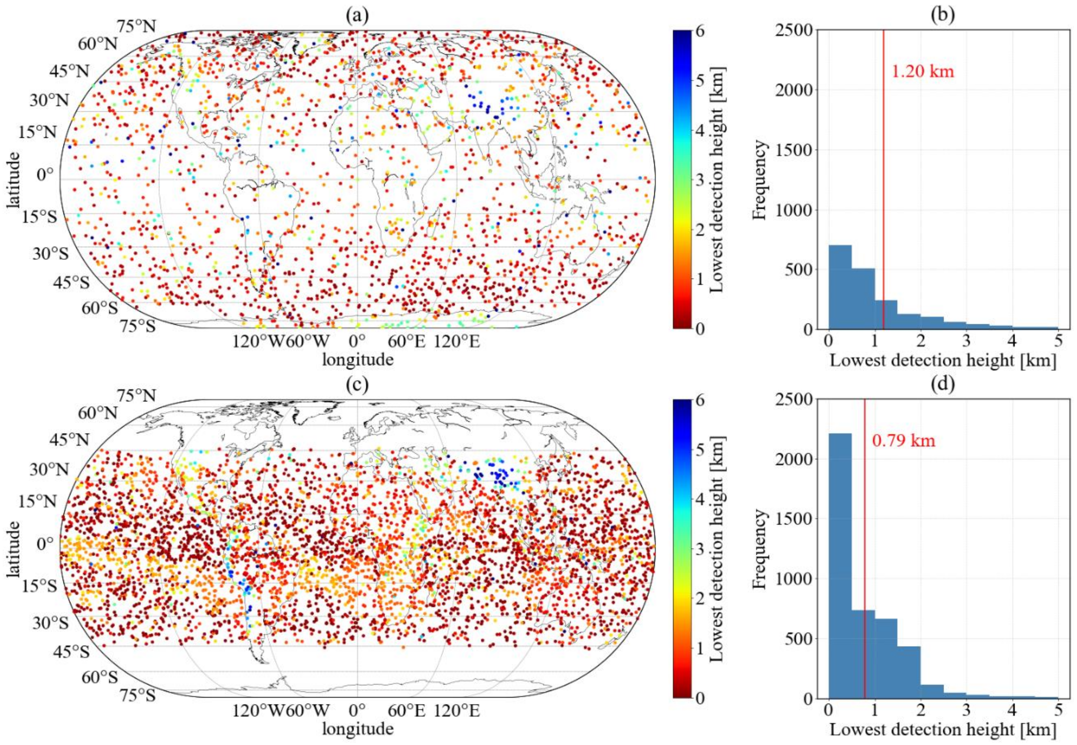
2.1. RO Data
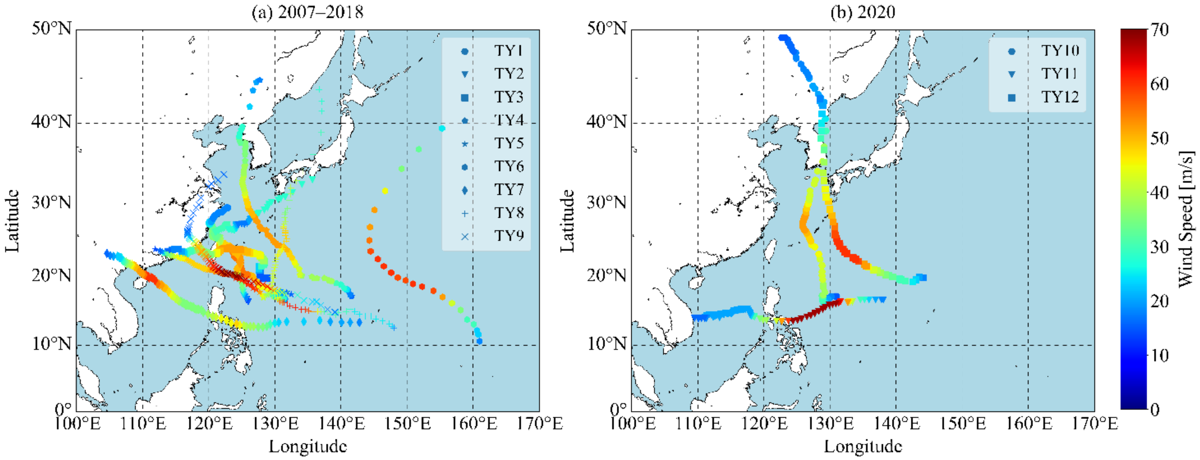
2.2. Typhoon Track
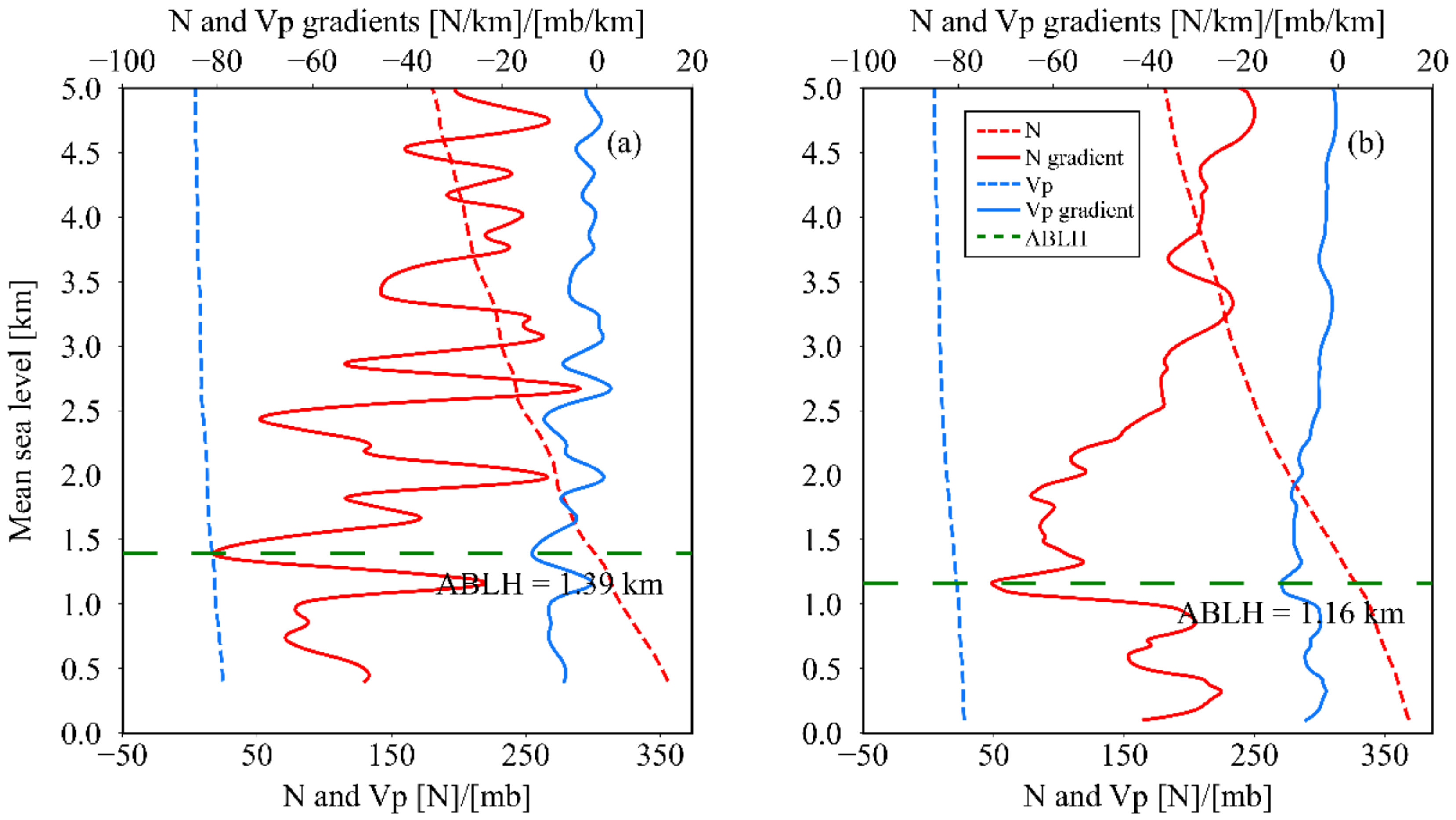
2.3. Algorithm for the ABLH
2.4. Method for Constructing ABLH Climatology
2.5. Co-Location of Typhoon and RO Profiles
3. Analysis Results
3.1. ABLH Climatology in Typhoon Season
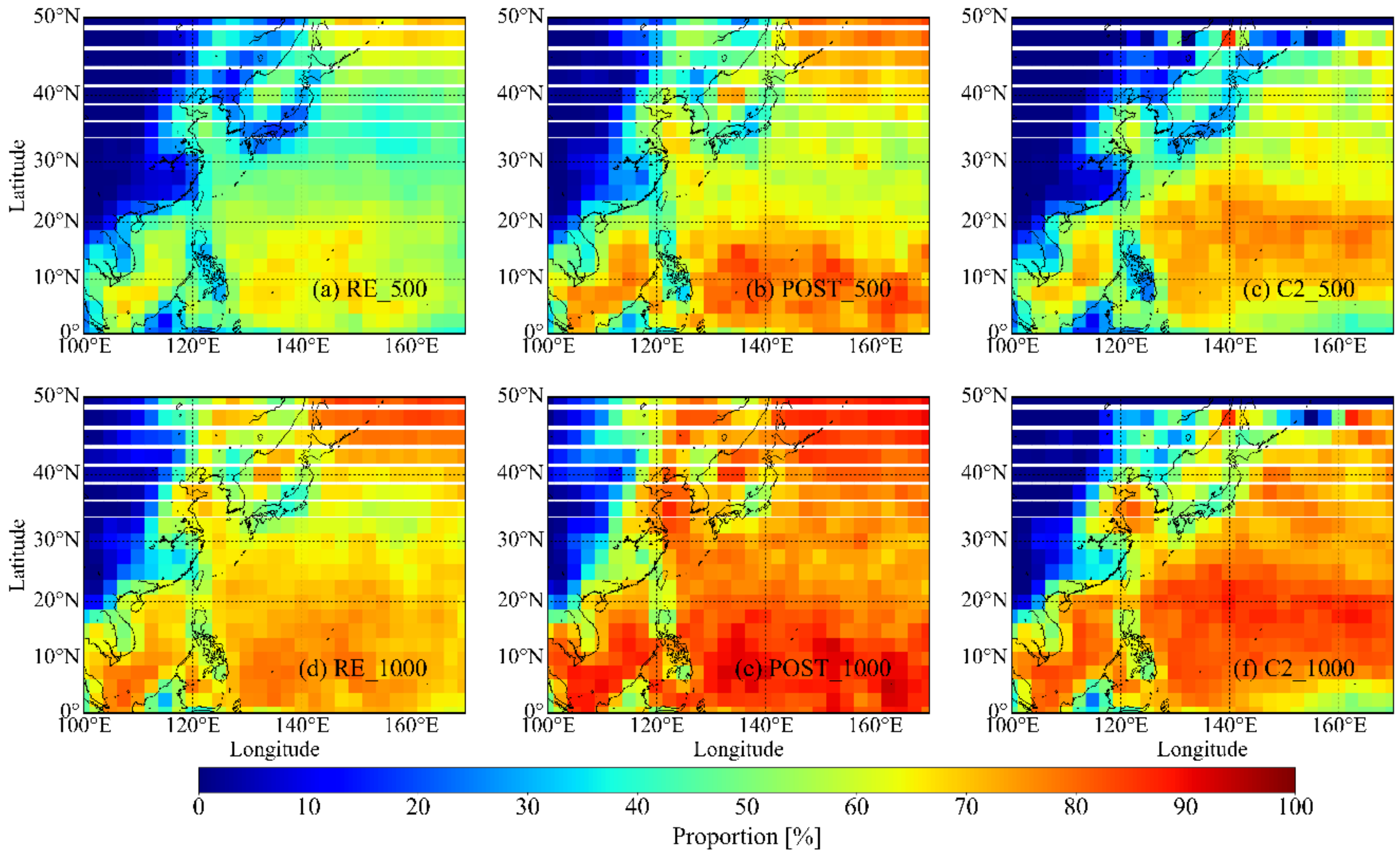
3.2. Co-Location Results Based on Various Time Windows
3.3. Mean ABLH in Typhoons
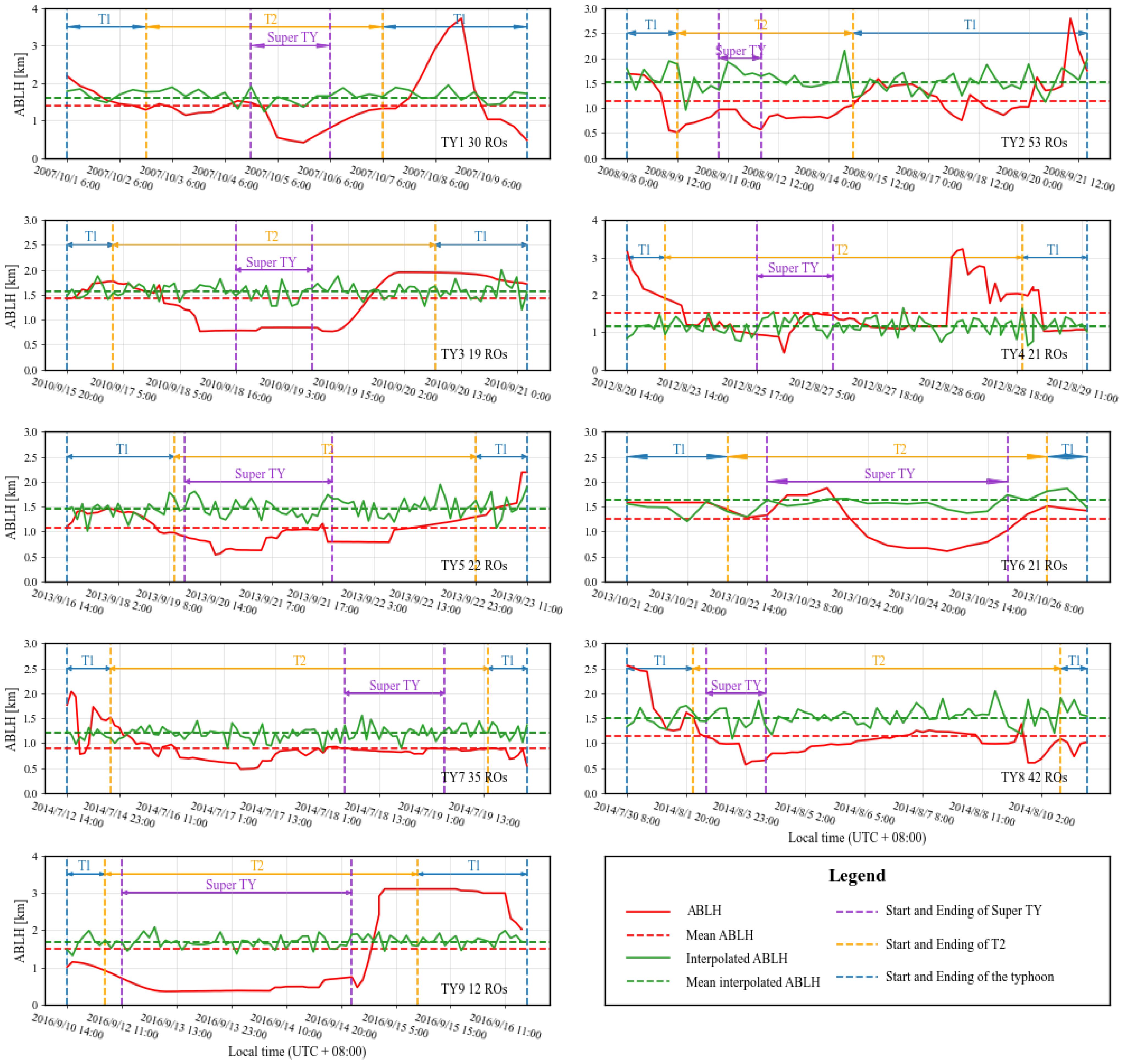
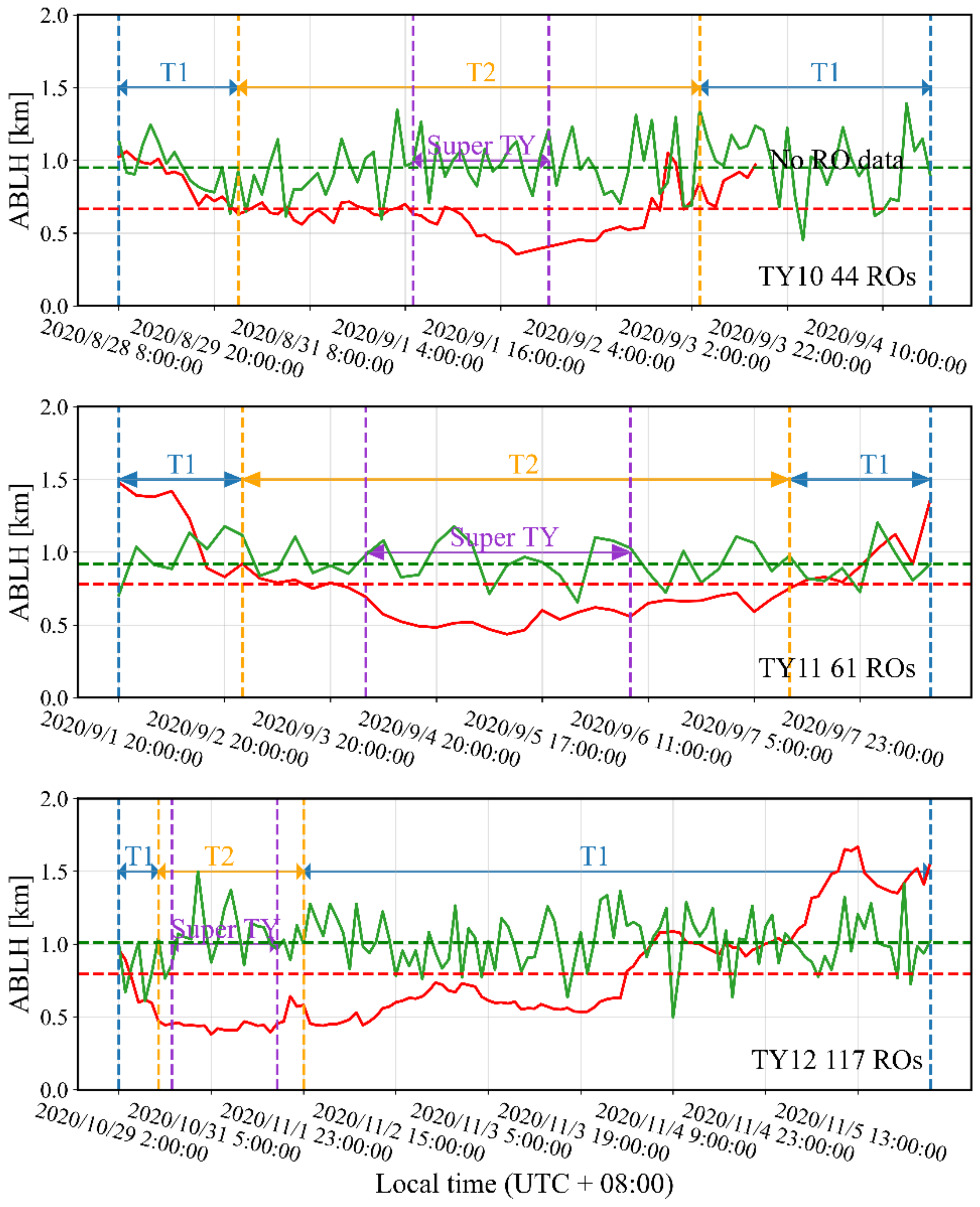
3.4. Variation in ABLH along Typhoon Track
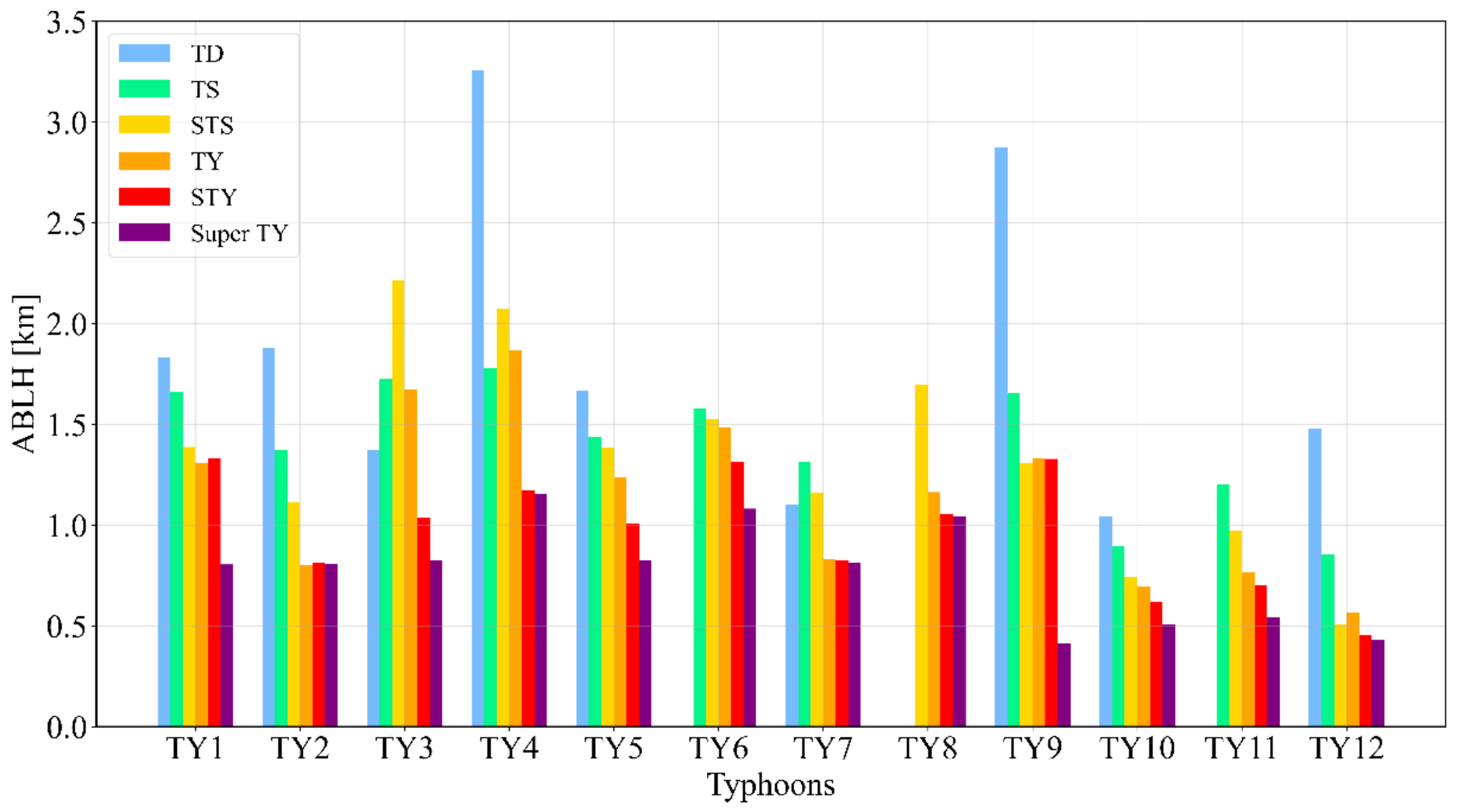
3.5. Mean ABLH at Different Stages of Typhoons
3.6. Correlation Analysis between the ABLH and Wind Speed
4. Discussion and Conclusions
Author Contributions
Funding
Institutional Review Board Statement
Informed Consent Statement
Data Availability Statement
Acknowledgments
Conflicts of Interest
References
- Ao, C.O.; Waliser, D.E.; Chan, S.K.; Li, J.-L.; Tian, B.; Xie, F.; Mannucci, A.J. Planetary boundary layer heights from GPS radio occultation refractivity and humidity profiles. J. Geophys. Res. Atmos. 2012, 117, D16117. [Google Scholar] [CrossRef] [Green Version]
- Emanuel, K. An Air-Sea Interaction Theory for Tropical Cyclones. Part I: Steady-State Maintenance. J. Atmos. Sci. 1986, 43, 585–605. [Google Scholar] [CrossRef]
- Wroe, D.; Barnes, G. Inflow Layer Energetics of Hurricane Bonnie (1998) near Landfall. Mon. Weather Rev. 2003, 131, 1600–1612. [Google Scholar] [CrossRef]
- Smith, R.; Montgomery, M.; Vogl, S. A critique of Emanuel’s hurricane model and potential intensity theory. Q. J. R. Meteorol. Soc. 2008, 134, 551–561. [Google Scholar] [CrossRef] [Green Version]
- Zhang, J.A.; Rogers, R.F.; Nolan, D.S.; Marks, F.D. On the Characteristic Height Scales of the Hurricane Boundary Layer. Mon. Weather Rev. 2011, 139, 2523–2535. [Google Scholar] [CrossRef]
- Seidel, D.J.; Ao, C.O.; Li, K. Estimating climatological planetary boundary layer heights from radiosonde observations: Comparison of methods and uncertainty analysis. J. Geophys. Res. 2010, 115, D16113. [Google Scholar] [CrossRef] [Green Version]
- Braun, S.; Tao, W.-K. Sensitivity of High-Resolution Simulations of Hurricane Bob (1991) to Planetary Boundary Layer Parameterizations. Mon. Weather Rev. 2000, 128, 3941–3961. [Google Scholar] [CrossRef] [Green Version]
- Smith, R.; Thomsen, G. Dependence of tropical-cyclone intensification on the boundary-layer representation in a numerical model. Q. J. R. Meteorol. Soc. 2010, 136, 1671–1685. [Google Scholar] [CrossRef]
- Ren, Y.; Zhang, J.A.; Guimond, S.R.; Wang, X. Hurricane Boundary Layer Height Relative to Storm Motion from GPS Dropsonde Composites. Atmosphere 2019, 10, 339. [Google Scholar] [CrossRef] [Green Version]
- Holzworth, C.G. Estimates of Mean Maximum Mixing Depths in the Contiguous United States. Mon. Weather Rev. 1964, 92, 235–242. [Google Scholar] [CrossRef] [Green Version]
- Beyrich, F. Mixing height estimation from sodar data—A critical discussion. Atmos. Environ. 1997, 31, 3941–3953. [Google Scholar] [CrossRef]
- Dupont, E.; Menut, L.; Carissimo, B.; Pelon, J.; Flamant, P. Comparison between the atmospheric boundary layer in Paris and its rural suburbs during the ECLAP experiment. Atmos. Environ. 1999, 33, 979–994. [Google Scholar] [CrossRef]
- Smith, A.B.; Katz, R.W. US billion-dollar weather and climate disasters: Data sources, trends, accuracy and biases. Nat. Hazards 2013, 67, 387–410. [Google Scholar] [CrossRef]
- Zhang, J.A.; Rogers, R.F.; Reasor, P.D.; Uhlhorn, E.W.; Marks, F.D. Asymmetric Hurricane Boundary Layer Structure from Dropsonde Composites in Relation to the Environmental Vertical Wind Shear. Mon. Weather Rev. 2013, 141, 3968–3984. [Google Scholar] [CrossRef]
- Smith, R.K.; Montgomery, M.T.; Van Sang, N. Tropical cyclone spin-up revisited. Q. J. R. Meteorol. Soc. 2009, 135, 1321–1335. [Google Scholar] [CrossRef] [Green Version]
- Kepert, J.D.; Schwendike, J.; Ramsay, H. Why is the Tropical Cyclone Boundary Layer Not “Well Mixed”? J. Atmos. Sci. 2016, 73, 957–973. [Google Scholar] [CrossRef]
- Bryan, G.H.; Rotunno, R. The Maximum Intensity of Tropical Cyclones in Axisymmetric Numerical Model Simulations. Mon. Weather Rev. 2009, 137, 1770–1789. [Google Scholar] [CrossRef]
- Zawislak, J.; Jiang, H.; Alvey, G.R.; Zipser, E.J.; Rogers, R.F.; Zhang, J.A.; Stevenson, S.N. Observations of the Structure and Evolution of Hurricane Edouard (2014) during Intensity Change. Part I: Relationship between the Thermodynamic Structure and Precipitation. Mon. Weather Rev. 2016, 144, 3333–3354. [Google Scholar] [CrossRef]
- Rogers, R.F.; Zhang, J.A.; Zawislak, J.; Jiang, H.; Alvey, G.R.; Zipser, E.J.; Stevenson, S.N. Observations of the Structure and Evolution of Hurricane Edouard (2014) during Intensity Change. Part II: Kinematic Structure and the Distribution of Deep Convection. Mon. Weather Rev. 2016, 144, 3355–3376. [Google Scholar] [CrossRef]
- Ooyama, K. Numerical Simulation of the Life Cycle of Tropical Cyclones. J. Atmos. Sci. 1969, 26, 3–40. [Google Scholar] [CrossRef]
- Schubert, W.H.; Hack, J.J. Inertial Stability and Tropical Cyclone Development. J. Atmos. Sci. 1982, 39, 1687–1697. [Google Scholar] [CrossRef]
- Coulter, R. A Comparison of Three Methods for Measuring Mixing-Layer Height. J. Appl. Meteorol. 1979, 18, 1495–1499. [Google Scholar] [CrossRef] [Green Version]
- Lokoshchenko, M. Long-Term Sodar Observations in Moscow and a New Approach to Potential Mixing Determination by Radiosonde Data. J. Atmos. Ocean. Technol. 2002, 19, 1151–1162. [Google Scholar] [CrossRef]
- Hock, T.; Franklin, J. The NCAR GPS dropwindesonde. Bull. Am. Meteorol. Soc. 1999, 80, 407–420. [Google Scholar] [CrossRef] [Green Version]
- Ratnam, M.V.; Basha, S.G. A robust method to determine global distribution of atmospheric boundary layer top from COSMIC GPS RO measurements. Atmos. Sci. Lett. 2010, 11, 216–222. [Google Scholar] [CrossRef]
- Guimond, S.; Tian, L.; Heymsfield, G.; Frasier, S.J. Wind Retrieval Algorithms for the IWRAP and HIWRAP Airborne Doppler Radars with Applications to Hurricanes. J. Atmos. Ocean. Technol. 2014, 31, 1189–1215. [Google Scholar] [CrossRef] [Green Version]
- Guimond, S.; Zhang, J.; Sapp, J.; Frasier, S.J. Coherent Turbulence in the Boundary Layer of Hurricane Rita (2005) During an Eyewall Replacement Cycle. J. Atmos. Sci. 2018, 75, 3071–3093. [Google Scholar] [CrossRef]
- Kursinski, E.R.; Hajj, G.A.; Schofield, J.T.; Linfield, R.P.; Hardy, K.R. Observing Earth’s atmosphere with radio occultation measurements using the Global Positioning System. J. Geophys. Res. Atmos. 1997, 102, 23429–23465. [Google Scholar] [CrossRef]
- Steiner, A.K.; Lackner, B.C.; Ladstädter, F.; Scherllin-Pirscher, B.; Foelsche, U.; Kirchengast, G. GPS radio occultation for climate monitoring and change detection. Radio Sci. 2011, 46, RS0D24. [Google Scholar] [CrossRef] [Green Version]
- Hajj, G.; Kursinski, R.; Romans, L.J.; Bertiger, W.I.; Leroy, S. A technical description of atmospheric sounding by GPS occultation. J. Atmos. Sol.-Terr. Phys. 2002, 64, 451–469. [Google Scholar] [CrossRef]
- Anthes, R.A. Exploring earth’s atmosphere with radio occultation: Contributions to weather, climate and space weather. Atmos. Meas. Tech. 2011, 4, 1077–1103. [Google Scholar] [CrossRef] [Green Version]
- Schreiner, W.; Sokolovskiy, S.; Hunt, D.; Rocken, C.; Kuo, Y.H. Analysis of GPS radio occultation data from the FORMOSAT-3/COSMIC and Metop/GRAS missions at CDAAC. Atmos. Meas. Tech. 2011, 4, 2255–2272. [Google Scholar] [CrossRef] [Green Version]
- Chen, S.-Y.; Liu, C.-Y.; Huang, C.-Y.; Hsu, S.-C.; Li, H.-W.; Lin, P.-H.; Cheng, J.-P.; Huang, C.-Y. An analysis study of FORMOSAT-7/COSMIC-2 radio occultation data in the troposphere. Remote Sens. 2021, 13, 717. [Google Scholar] [CrossRef]
- Ho, S.-P.; Zhou, X.; Shao, X.; Zhang, B.; Adhikari, L.; Kireev, S.; He, Y.; Yoe, J.G.; Xia-Serafino, W.; Lynch, E. Initial Assessment of the COSMIC-2/FORMOSAT-7 Neutral Atmosphere Data Quality in NESDIS/STAR Using In Situ and Satellite Data. Remote Sens. 2020, 12, 4099. [Google Scholar] [CrossRef]
- Schreiner, W.S.; Weiss, J.P.; Anthes, R.A.; Braun, J.; Chu, V.; Fong, J.; Hunt, D.; Kuo, Y.-H.; Meehan, T.; Serafino, W.; et al. COSMIC-2 Radio Occultation Constellation: First Results. Geophys. Res. Lett. 2020, 47, e2019GL086841. [Google Scholar] [CrossRef]
- Biondi, R.; Ho, S.-P.; Randel, W.; Syndergaard, S.; Neubert, T. Tropical cyclone cloud-top height and vertical temperature structure detection using GPS radio occultation measurements. J. Geophys. Res. Atmos. 2013, 118, 5247–5259. [Google Scholar] [CrossRef]
- Biondi, R.; Steiner, A.K.; Kirchengast, G.; Rieckh, T. Characterization of thermal structure and conditions for overshooting of tropical and extratropical cyclones with GPS radio occultation. Atmos. Chem. Phys. 2015, 15, 5181–5193. [Google Scholar] [CrossRef] [Green Version]
- Ravindra Babu, S.; Venkat Ratnam, M.; Basha, G.; Krishnamurthy, B.V.; Venkateswararao, B. Effect of tropical cyclones on the tropical tropopause parameters observed using COSMIC GPS RO data. Atmos. Chem. Phys. 2015, 15, 10239–10249. [Google Scholar] [CrossRef] [Green Version]
- Lasota, E.; Steiner, A.K.; Kirchengast, G.; Biondi, R. Tropical cyclones vertical structure from GNSS radio occultation: An archive covering the period 2001–2018. Earth Syst. Sci. Data 2020, 12, 2679–2693. [Google Scholar] [CrossRef]
- Xie, F.; Wu, D.L.; Ao, C.O.; Mannucci, A.J.; Kursinski, E.R. Advances and limitations of atmospheric boundary layer observations with GPS occultation over southeast Pacific Ocean. Atmos. Chem. Phys. 2012, 12, 903–918. [Google Scholar] [CrossRef] [Green Version]
- Basha, G.; Kishore, P.; Ratnam, M.V.; Ravindra Babu, S.; Velicogna, I.; Jiang, J.H.; Ao, C.O. Global climatology of planetary boundary layer top obtained from multi-satellite GPS RO observations. Clim. Dyn. 2018, 52, 2385–2398. [Google Scholar] [CrossRef]
- Bonafoni, S.; Biondi, R.; Brenot, H.; Anthes, R. Radio occultation and ground-based GNSS products for observing, understanding and predicting extreme events: A review. Atmos. Res. 2019, 230, 104624. [Google Scholar] [CrossRef]
- Ao, O.; Hajj, G.; Meehan, T.; Dong, D.; Iijima, B.; Mannucci, A.; Kursinski, R. Rising and Setting GPS Occultations by Use of Open-Loop Tracking. J. Geophys. Res. 2009, 114. [Google Scholar] [CrossRef] [Green Version]
- Ho, S.-P.; Anthes, R.A.; Ao, C.O.; Healy, S.; Horanyi, A.; Hunt, D.; Mannucci, A.J.; Pedatella, N.; Randel, W.J.; Simmons, A.; et al. The COSMIC/FORMOSAT-3 Radio Occultation Mission after 12 Years: Accomplishments, Remaining Challenges, and Potential Impacts of COSMIC-2. Bull. Am. Meteorol. Soc. 2020, 101, E1107–E1136. [Google Scholar] [CrossRef] [Green Version]
- Hordyniec, P.; Kuleshov, Y.; Choy, S.; Norman, R. Observation of Deep Occultation Signals in Tropical Cyclones with COSMIC-2 Measurements. IEEE Geosci. Remote Sens. Lett. 2021, 1–5. [Google Scholar] [CrossRef]
- Sokolovskiy, S.V.; Rocken, C.; Lenschow, D.H.; Kuo, Y.H.; Anthes, R.A.; Schreiner, W.S.; Hunt, D.C. Observing the moist troposphere with radio occultation signals from COSMIC. Geophys. Res. Lett. 2007, 34, L18802. [Google Scholar] [CrossRef] [Green Version]
- Basha, G.; Ratnam, M.V. Identification of atmospheric boundary layer height over a tropical station using high-resolution radiosonde refractivity profiles: Comparison with GPS radio occultation measurements. J. Geophys. Res. Atmos. 2009, 114. [Google Scholar] [CrossRef]
- Yan, S.; Xiang, J.; Du, H. Determining Atmospheric Boundary Layer Height with the Numerical Differentiation Method Using Bending Angle Data from COSMIC. Adv. Atmos. Sci. 2019, 36, 303–312. [Google Scholar] [CrossRef]
- Peevey, T.R.; Atlas, R.; Hoffman, R.N.; Casey, S.P.F.; Cucurull, L.; Kren, A.C.; Mueller, M.J. Impact of Refractivity Profiles from a Proposed GNSS-RO Constellation on Tropical Cyclone Forecasts in a Global Modeling System. Mon. Weather Rev. 2020, 148, 3037–3057. [Google Scholar] [CrossRef]
- Smith, E.K.; Weintraub, S. The Constants in the Equation for Atmospheric Refractive Index at Radio Frequencies. Proc. IRE 1953, 50, 1035–1037. [Google Scholar] [CrossRef] [Green Version]
- Melbourne, W.G.; Davis, E.S.; Duncan, C.B. The Application of Spaceborne GPS to Atmospheric Limb Sounding and Global Change Monitoring; NASA Jet Propulsion Laboratory: Pasadena, CA, USA, 1994; pp. 4–18.
- Stull, R.B. An Introduction to Boundary Layer Meteorology, 1st ed.; Springer: Dordrecht, The Netherlands, 1988; p. I-1. [Google Scholar]
- Brunner, L.; Steiner, A.K.; Scherllin-Pirscher, B.; Jury, M.W. Exploring atmospheric blocking with GPS radio occultation observations. Atmos. Chem. Phys. 2016, 16, 4593–4604. [Google Scholar] [CrossRef] [Green Version]


| Scale | Tropical Depression | Tropical Storm | Severe Tropical Storm | Typhoon | Severe Typhoon | Super Typhoon |
|---|---|---|---|---|---|---|
| Abbreviation | TD | TS | STS | TY | STY | Super TY |
| Wind speed | 10.8–17.1 | 17.1–24.4 | 24.4–32.6 | 32.6–41.4 | 41.4–51 | ≥51 |
| Typhoon | Time (UTC+8) | Starting Position | Ending Position | Max Wind Speed (m/s) | Num. of Positions |
|---|---|---|---|---|---|
| TY1, Krosa | 2007/10/02–2007/10/08 | 130.0° 17.1° | 122.9° 29.5° | 55 | 103 |
| TY2, Sinlaku | 2008/09/08–2008/09/19 | 126.0° 16.4° | 135.7° 33.1° | 52 | 171 |
| TY3, Fanapi | 2010/09/15–2010/09/21 | 128.8° 19.8° | 113.8° 23.6° | 52 | 97 |
| TY4, Bolaven | 2012/08/20–2012/08/29 | 141.6° 17.2° | 127.7° 44.8° | 52 | 82 |
| TY5, Usagi | 2013/09/16–2013/09/23 | 132.5° 17.5° | 111.9° 23.9° | 60 | 91 |
| TY6, Lekima | 2013/10/21–2013/10/26 | 161.0° 10.6° | 155.3° 39.4° | 60 | 24 |
| TY7, Rammasun | 2014/07/12–2014/07/20 | 142.8° 13.4° | 104.6° 23.3° | 60 | 107 |
| TY8, Halong | 2014/07/29–2014/08/11 | 148.0° 12.6° | 136.7° 43.8° | 62 | 75 |
| TY9, Meranti | 2016/09/10–2016/09/16 | 139.1° 14.9° | 122.3° 33.8° | 70 | 85 |
| TY10, Maysak | 2020/08/28–2020/09/04 | 131.0° 17.2° | 122.7° 49.2° | 52 | 103 |
| TY11, Haishen | 2020/09/01–2020/09/08 | 144.1° 19.9° | 128.5° 48.2° | 60 | 47 |
| TY12, Goni | 2020/10/29–2020/11/06 | 138.1° 16.7° | 109.5° 14.0° | 68 | 124 |
| Typhoon | Time Window | |||||||||||
|---|---|---|---|---|---|---|---|---|---|---|---|---|
| 6 h | 12 h | 18 h | 24 h | 30 h | 36 h | |||||||
| Num | % | Num | % | Num | % | Num | % | Num | % | Num | % | |
| TY1 | 12 | 42 | 15 | 56 | 18 | 67 | 22 | 78 | 27 | 86 | 30 | 89 |
| TY2 | 28 | 57 | 26 | 80 | 41 | 91 | 44 | 98 | 49 | 100 | 53 | 100 |
| TY3 | 10 | 45 | 10 | 63 | 11 | 77 | 12 | 88 | 17 | 95 | 19 | 100 |
| TY4 | 9 | 44 | 11 | 67 | 12 | 86 | 17 | 98 | 19 | 100 | 21 | 100 |
| TY5 | 14 | 54 | 16 | 76 | 16 | 82 | 19 | 89 | 21 | 99 | 22 | 100 |
| TY6 | 4 | 21 | 8 | 50 | 10 | 63 | 13 | 75 | 18 | 92 | 21 | 96 |
| TY7 | 14 | 59 | 19 | 71 | 22 | 89 | 26 | 100 | 31 | 100 | 35 | 100 |
| TY8 | 20 | 54 | 26 | 70 | 30 | 79 | 33 | 87 | 38 | 94 | 42 | 96 |
| TY9 | 4 | 15 | 5 | 26 | 7 | 38 | 8 | 48 | 9 | 62 | 12 | 76 |
| Average % | 43 | 62 | 75 | 85 | 92 | 95 | ||||||
| RO | COSMIC | COSMIC-2 | ||||||||||||
|---|---|---|---|---|---|---|---|---|---|---|---|---|---|---|
| TY | TY1 | TY2 | TY3 | TY4 | TY5 | TY6 | TY7 | TY8 | TY9 | Mean1 | TY10 | TY11 | TY12 | Mean2 |
| T1 | 2.02 | 1.18 | 2.07 | 2.51 | 1.44 | 1.50 | 0.89 | 1.70 | 2.10 | 1.71 | 0.87 | 1.09 | 0.87 | 0.94 |
| T2 | 0.97 | 0.88 | 1.01 | 1.75 | 0.86 | 1.20 | 0.71 | 1.11 | 0.47 | 0.99 | 0.59 | 0.64 | 0.46 | 0.56 |
| T1–T2 | 1.05 | 0.31 | 1.07 | 0.76 | 0.58 | 0.30 | 0.18 | 0.59 | 1.63 | 0.72 | 0.28 | 0.45 | 0.41 | 0.38 |
| TY | TY1 | TY2 | TY3 | TY4 | TY5 | TY6 | TY7 | TY8 | TY9 | TY10 | TY11 | TY12 |
|---|---|---|---|---|---|---|---|---|---|---|---|---|
| TY_YEAR | 1.40 | 1.13 | 1.44 | 1.53 | 1.08 | 1.26 | 0.89 | 1.14 | 1.49 | 0.67 | 0.78 | 0.79 |
| NO_TY | 1.59 | 1.52 | 1.57 | 1.17 | 1.45 | 1.63 | 1.21 | 1.51 | 1.69 | 0.95 | 0.92 | 1.01 |
| DIF | −0.19 | −0.39 | −0.13 | 0.36 | −0.37 | −0.37 | −0.32 | −0.37 | −0.20 | −0.28 | −0.14 | −0.22 |
Publisher’s Note: MDPI stays neutral with regard to jurisdictional claims in published maps and institutional affiliations. |
© 2021 by the authors. Licensee MDPI, Basel, Switzerland. This article is an open access article distributed under the terms and conditions of the Creative Commons Attribution (CC BY) license (https://creativecommons.org/licenses/by/4.0/).
Share and Cite
Shi, J.; Zhang, K.; Wu, S.; Shi, S.; Shen, Z. Investigation of the Atmospheric Boundary Layer Height Using Radio Occultation: A Case Study during Twelve Super Typhoons over the Northwest Pacific. Atmosphere 2021, 12, 1457. https://doi.org/10.3390/atmos12111457
Shi J, Zhang K, Wu S, Shi S, Shen Z. Investigation of the Atmospheric Boundary Layer Height Using Radio Occultation: A Case Study during Twelve Super Typhoons over the Northwest Pacific. Atmosphere. 2021; 12(11):1457. https://doi.org/10.3390/atmos12111457
Chicago/Turabian StyleShi, Jiaqi, Kefei Zhang, Suqin Wu, Shuangshuang Shi, and Zhen Shen. 2021. "Investigation of the Atmospheric Boundary Layer Height Using Radio Occultation: A Case Study during Twelve Super Typhoons over the Northwest Pacific" Atmosphere 12, no. 11: 1457. https://doi.org/10.3390/atmos12111457
APA StyleShi, J., Zhang, K., Wu, S., Shi, S., & Shen, Z. (2021). Investigation of the Atmospheric Boundary Layer Height Using Radio Occultation: A Case Study during Twelve Super Typhoons over the Northwest Pacific. Atmosphere, 12(11), 1457. https://doi.org/10.3390/atmos12111457