Article

Basic Facts about Numerical Simulations of Atmospheric Composition in the City of Sofia

National Institute of Geophysics, Geodesy and Geography, Bulgarian Academy of Sciences, Acad. G. Bonchev Str., Bl. 3, 1113 Sofia, Bulgaria
*
Author to whom correspondence should be addressed.
Atmosphere 2021, 12(11), 1450; https://doi.org/10.3390/atmos12111450
Submission received: 30 September 2021 / Revised: 25 October 2021 / Accepted: 28 October 2021 / Published: 2 November 2021

Abstract

:
The atmospheric composition in urban areas is one of the primary tasks in air pollution studies. The research aims to provide a statistically reliable assessment of the atmospheric composition climate of the city of Sofia—typical and extreme features of the special/temporal behavior, annual means, seasonal and diurnal variations. For that purpose, extensive numerical simulations of the atmospheric composition fields in Sofia city have been performed. Three models were chosen as modeling tools. We used WRF as a meteorological pre-processor, CMAQ as a chemical transport model, and SMOKE as the emission pre-processor of Models-3 system. We developed the following conclusions. The daily concentration changes of the two essential air pollution species—nitrogen dioxide (NO2) and fine particle matters (FPRM, particulate matter (PM2.5), which has a diameter between 0 and 2.5 micrometers)—have different magnitudes. Second, the emissions relative contributions to the concentration of different species could be different, varying from 0% to above 100%. The contributions of different emission categories to other species surface concentrations have various diurnal courses. Last, the total concentration change (ΔC) is different for each pollutant. The sign of the contributions of some processes is evident. Still, some may have different signs depending on the type of emissions, weather conditions, or topography.

1. Introduction

The atmospheric composition in urban areas is one of the primary tasks in air pollution studies. The air pollution climate in urban areas has not been systematically studied yet in Bulgaria, but some air pollution modeling for the city of Sofia had been performed, and air pollution forecast for the city is operationally occurring [1,2,3,4,5]. Recently, extensive studies for long enough simulation periods and reasonable resolution of the atmospheric composition status in Bulgaria have been carried out using up-to-date modeling tools and detailed and reliable input data [6,7,8,9,10,11,12,13,14,15,16,17,18,19,20,21,22,23,24,25]. The next step in studying the atmospheric composition climate is performing simulations on an urban scale. Research works dealing with this topic include domains with different sizes and scales from meters to kilometers [26,27,28,29,30,31,32,33,34]. The models’ simulations in the smallest scales usually deal with sub-urban-sized areas as streets and neighborhoods. The simulations aim to construct an ensemble comprehensive enough to provide a statistically reliable assessment of the atmospheric composition climate of the city of Sofia—typical and extreme features of the special/temporal behavior, annual means, seasonal and diurnal variations, etc. Some evaluations of the contribution of different pollution sources and dynamic and chemical processes to the atmospheric composition of the city of Sofia will be presented in the paper.
Methodology: Extensive numerical simulations of the atmospheric composition fields in Sofia city have been recently performed, and an ensemble, comprehensive enough as to provide a statistically reliable assessment of the atmospheric composition climate, was constructed. The US EPA Models-3 system was chosen as a modeling tool. WRF [35] used as meteorological pre-processor, CMAQ—the Community Multiscale Air Quality System [36,37], being the Chemical Transport Model (CTM) of the system, and SMOKE—the Sparse Matrix Operator Kernel Emissions Modeling System [38]—the emission pre-processor of Models-3 system.
As the NCEP Global Analysis Data with one-degree resolution is used as meteorological background, the system nesting capabilities were applied for downscaling the simulations to a 1 km resolution (Figure 1). Results for the Sofia city domain (D5) and two locations—Orlov most and Bistritsa—are presented in this paper. Orlov most is located in the center of the city and represents a typical urban-polluted site. Bistritsa is located on the semi-mountain outskirts and represents a rural site of the domain.
The TNO inventory with resolution 0.25° × 0.125° in 10 SNAP categories for 2010 [39,40,41] is exploited for the territories outside Bulgaria in the mother CMAQs domain. For the Bulgarian domains, the National inventory for 2010 as provided by Bulgarian Executive Environmental Agency is used. All simulations were performed for a 7-year period from 2008 to 2014 with two-way nesting mod on. Special pre-processing procedures were created for introducing temporal profiles and speciation of the emissions [42].
The study is based on a large number of numerical simulations carried out daily for all periods. Different characteristics of the numerically obtained concentration fields and for five emission scenarios, with all the emissions included and reduced of factor 0.8, including emissions from energetics, non-industrial and industrial combustions, and road transport, will be demonstrated in the present paper. Results concerning the contribution of the different emission categories are demonstrated. The air pollution pattern is also formed as a result of the interaction of different processes; thus, knowing the contribution of each one of these processes for different meteorological conditions and given emission spatial configuration and temporal profiles is useful for understanding the atmospheric composition and air pollutants origin and behavior. To analyze the contribution of different dynamic and chemical processes, the CMAQ “integrated process rate analysis” option was applied. The procedure allows the concentration change for each compound to be presented as a sum of the contribution of each one of the processes, which determines the air pollution concentration.

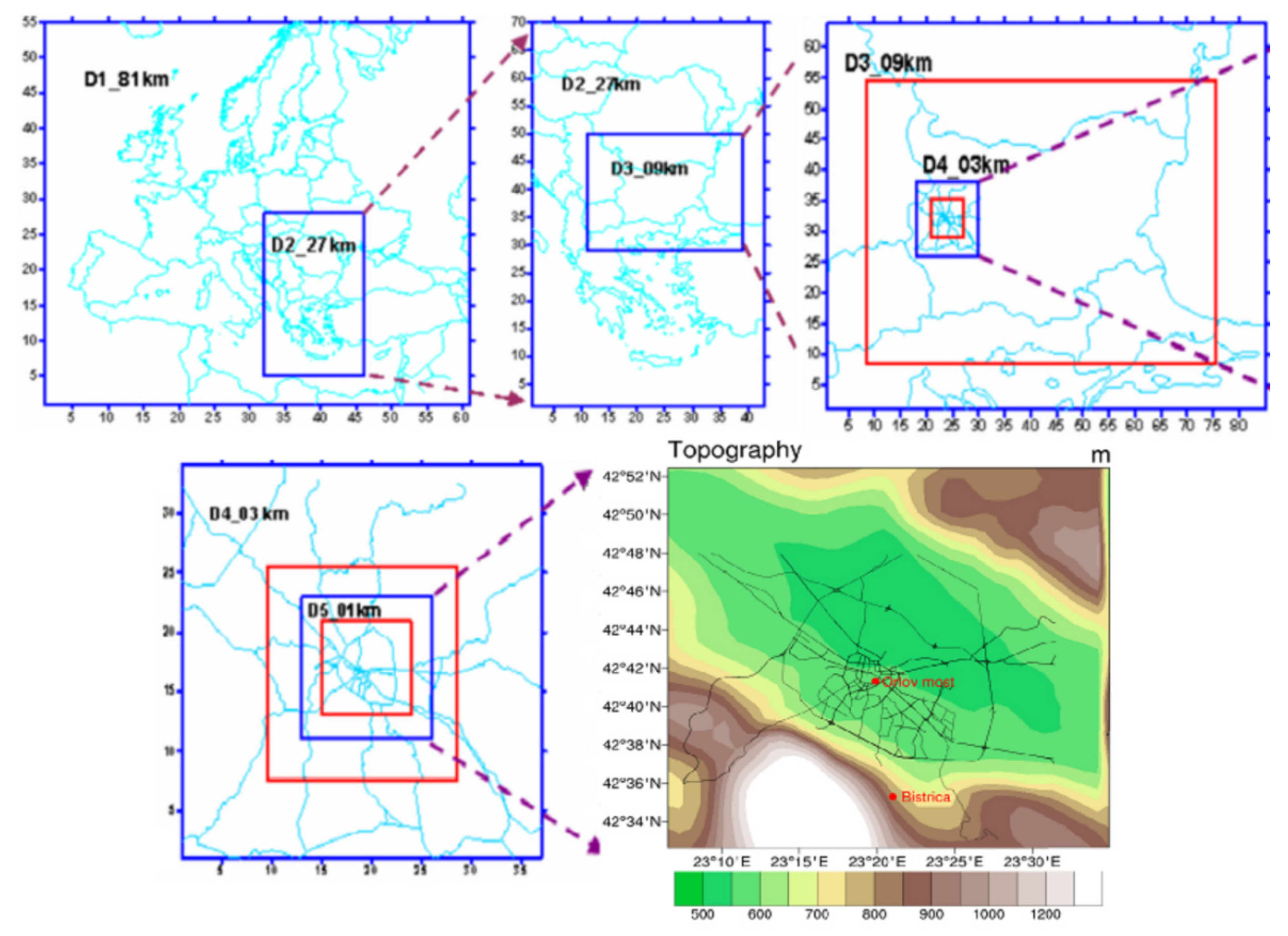
2. Materials and Methods

The sample size of the 7-year simulation is large and comprehensive enough to allow processing a variety of statistical quantities. We can calculate different statistics for the entire Sofia city domain, as well as for chosen locations—dispersion, the absolute minimum and maximum concentrations, a percent of the averages in the given interval of values, the probability density function, skewness, kurtosis, etc.
We present plots for the main statistical characteristics of the ensemble characteristics of the air pollution, namely seasonal and annual ones for some pollutants NO2 (nitrogen dioxide) and FPRM (fine particulate matter), averaged for the Sofia city region and in two locations in the city—Orlov most (point situated at the city center) and Bistrica (situated at semi-mountain outskirts). The plots give graphics of mean concentrations, maximum ones for entire simulation (period/ensemble), and curves noted as 10%, 25%, 75%, and 90%, for the 10th, 25th, 75th, and 90th percentile, respectively. The resulting curves suggest that 50% of the cases fall into the 25–75% interval, and 80% of the cases fall into the 10–90% interval. The plotted curves give a good enough idea for the statistical characteristics of the ensemble—dispersion, asymmetry, excess kurtosis, without being shown explicitly. The axes are given in logarithmic scale due to the high absolute minimal concentrations and the impossibility to distinguish the intervals of cases with different concentrations from the absolute ones on one plot. The absolute minimum concentrations are close to zero in most of the cases; thus, they are not shown on the logarithmic plots.
As already stated, the simulated fields ensemble is large enough to allow statistical treatment. In particular, the probability density functions for each of the atmospheric compounds can be calculated, with the respective seasonal and diurnal variations, for each of the points of the simulation grid or averaged over the territory of the city. Knowing the probability density functions means knowing everything about the ensemble. An example of spatial and diurnal variations of the annual ensembles of surface NO2 and FPRM behaviors ate two locations, the typically urban site “Orlov most” and “Bistritsa”, are shown in the paper.
The emission inventory, used in the simulations, includes 10 emission categories (SNAP categories) and allows the evaluation of the contribution of various anthropogenic activities to the overall picture of air pollution in the city of Sofia:
  • SNAP 1 (Combustion in energetics) reduced with factor 0.8;
  • SNAP 2 (Non-industrial combustion plants) reduced with factor 0.8;
  • SNAP 3 (Combustion in manufacturing industry) reduced with factor 0.8;
  • Production processes;
  • Extraction and distribution of fossil fuels;
  • Solvent and other product use;
  • SNAP 7 (Road transport) reduced with factor 0.8;
  • Other mobile sources and machinery;
  • Waste treatment and disposal;
  • Agriculture.
The used SNAP categorization of emissions, reduced by some factor, allows evaluation of the contribution of road transport, energetic, industrial, and non-industrial combustions to the atmospheric composition in the city. The concentrations for each scenario of reduced SNAP’s were calculated for each day of the period, and the relative contribution of the emissions for each of the scenarios was calculated in the following way.
If an arbitrary pollution characteristic (concentration, deposition, process contribution, etc.) for a given grid point, or averaged over chosen domain, obtained with all the emissions accounted for, is denoted by ϕ, then ϕm is the respective characteristic obtained when the emissions form source category m is reduced by a factor of α. In such a case, the quantity φm can be interpreted as the relative (in %) contributions of emission category m to the formation of the characteristic φ:
φ m =   1 1 α ϕ ϕ m ϕ · 100
More than one selected nomenclature for sources of air pollution (SNAP) category emissions can be reduced by a factor of α, and thus the joint contribution of several or all SNAP categories to the formation of the pollution characteristic ϕ can be evaluated. Obtained relative source contributions can also be averaged for the entire ensemble, thus providing the “climate” of the emission contributions, in particular the “typical” annual and seasonal contributions.
The reason why the emissions from a given category are reduced by a chosen factor and not simply at zero is that by completely removing the emissions from a given category, we can obtain much smaller concentrations, which may change the rate of some nonlinear chemical reactions. Moreover, the significant reduction of the concentrations may change the compound diffusion through the domain boundaries, which is why it is a general practice for the simulations to evaluate the contribution of emissions from a given category to be performed as applied and not removed, but reduced emissions from this category, which is normally performed in such studies. The reduction of 20% is preferred by many authors in atmospheric pollution studies.
Five emission scenarios will be considered here: Simulations with all the emissions included and with the emissions from all the SNAP categories (SNALL), SNAP categories 1 (energetics—SN1), SNAP categories 2 (non-industrial combustions—SN2), SNAP categories 3 (industrial combustions—SN3) and SNAP categories 7 (road transport—SN7) for Sofia reduced by a factor of 0.8. This makes it possible to evaluate the contribution of all the emissions, as well as the emissions from road transport, energetics, industrial and non-industrial combustions to the atmospheric composition in the city. The relative contribution of the emissions for each scenario was calculated for each day of this 7-year period, and then, by averaging over the ensemble, the typical fields of relative contributions of these emissions to the surface concentrations of each of the compounds were calculated for the four seasons and annually. For all the emission categories, the pattern of the contribution fields is complex, which reflects the emission source configuration, the heterogeneity of topography, land use, and meteorological conditions. In order to demonstrate the emission contribution behavior in a simpler and easy to comprehend way, the respective fields can be averaged over some domain, which makes it possible to follow and compare the diurnal behavior of the respective contributions for different species. Graphics of the diurnal evolution of the “typical” relative contribution annually and seasonal emissions of SNAP categories 1, 2, 3, 7 and all the emissions to the surface concentrations of NO2, FPRM, averaged for the territory of Sofia city and for Orlov most and Bistritsa, are shown in figures.
Atmospheric pollution is a result of the interaction of different dynamic and chemical processes. The consideration of the interaction and contribution of these processes provides a possibility for an explanation of the entire picture of the air pollution in Sofia city. The processes that influence the formation of the air pollution patterns are HADV—horizontal advection, ZADV—vertical advection, HDIF—horizontal diffusion, VDIF—vertical diffusion, EMIS—emissions, DDEP—dry deposition, CLDS—cloud processes, CHEM—chemical processes, and AERO—aerosol processes. In the current section, we present mainly results from the high-performance computing simulations, which evaluate the contribution of different dynamic transportation and transformation processes of air pollutants, which form the air pollution climate in Sofia city. The function of the CMAQ model—“integrated process rate analysis” was used for this task—a specific option that gives an opportunity to estimate the role of each one of the former processes in air pollution formation. In that way, the concentration change ΔCi of the i-th pollutant for a given time interval from t to [t+ Δt], can be present as a sum of the contributions of the different processes that determine the concentration change, i.e., the equation for transport and transformation of pollutants can be written in the form:
Δ c i 1   =   ( Δ c i 1 ) h d i f   +   ( Δ c i 1 ) v d i f   +   ( Δ c i 1 ) h   a d v   +   ( Δ c i 1 ) v   a d v   +   ( Δ c i 1 ) d r y d e p +   ( Δ c i 1 ) e m i s s   +   ( Δ c i 1 ) c h e m   +   ( Δ c i 1 ) c l o u d   +   ( Δ c i 1 ) a e r o
The figures show the annual and seasonal averaged contributions of the HADV, ZADV, HDIF, VDIF, EMIS, DDEP, CLDS, CHEM, AERO leading to the different air pollutants (NO2, FPRM) formations, averaged for some locations of the domain, as well as for the entire one—Sofia city. All the plots demonstrated are for the first model layer. The total change of the concentration (ΔC) is also plotted, and we can see its sign—positive or negative and that it has a well pronounced diurnal course. Different contributions with different values dominate the formation of the air pollutants, which is traced on the graphics and which contribution of given processes dominate, in a given time and sign.

3. Results

The Section 3 is separated into three parts and presents characteristics of the numerically obtained concentration fields, the contribution of different emission sources, and process analysis of the atmospheric composition for the entire domain Sofia city and two locations—Orlov most and Bistritsa.
Graphics of the diurnal evolution of the “typical” relative contribution—annual and seasonal emissions—of SNAP categories 1, 2, 3, 7 and the emissions of the surface concentrations of NO2 and FPRM, averaged for the territory of Sofia city and for Orlov most and Bistritsa, are shown.
The annual and seasonal averaged contributions of the processes leading to the formation of pollutants (NO2, FPRM), averaged for some locations of the domain as well as for the entire Sofia city, are presented. The total change of the concentration (ΔC) is also plotted, and we can see its sign—positive or negative—has a well pronounced diurnal course. Different contributions with different values dominate the formation of the air pollutants, which is traced on the graphics—where a given process dominates, at a given time and sign. The values of ΔC differ in different seasons and are defined from the superposition of the contributions of the different processes, which are also with a different signs.

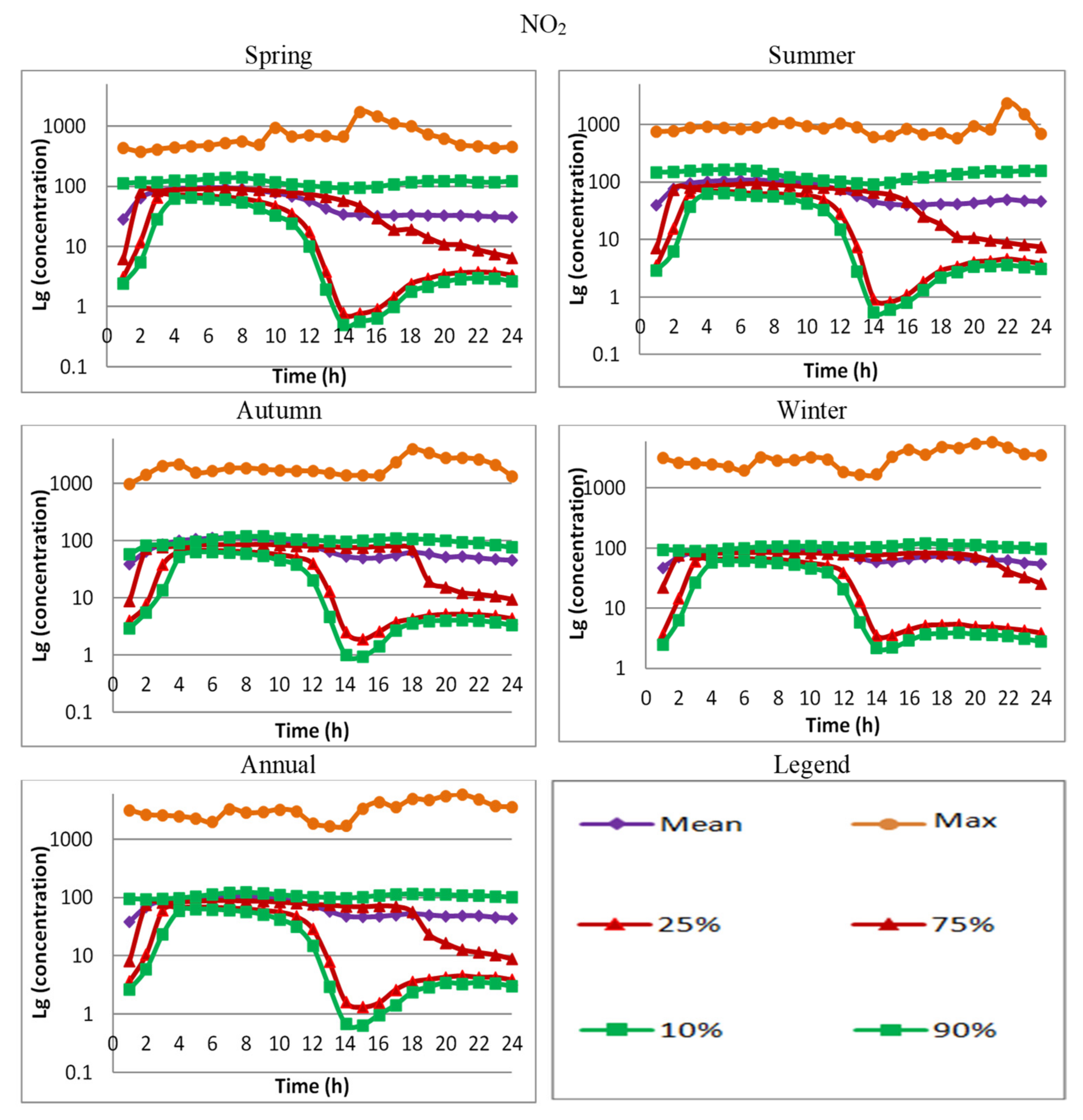
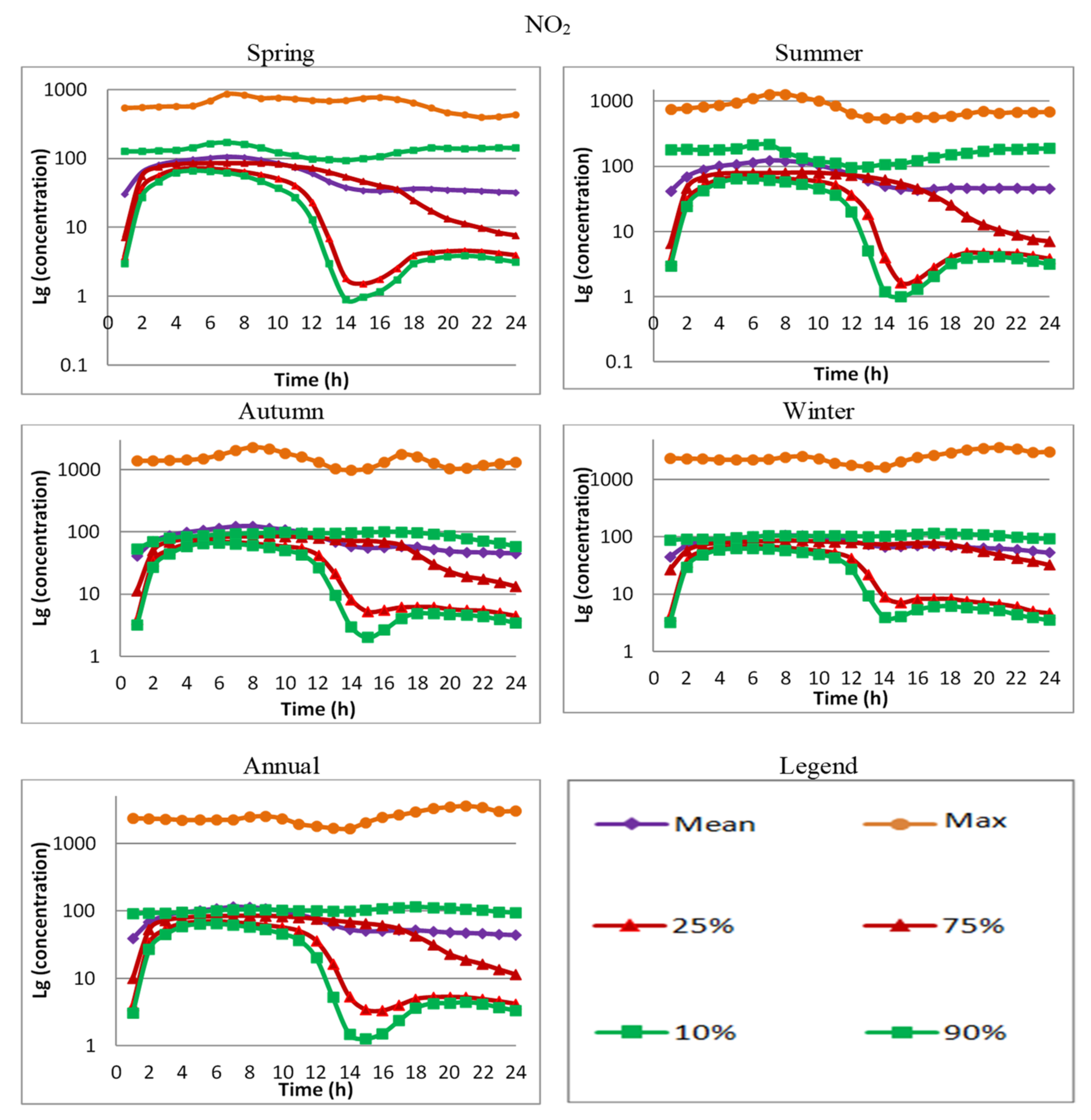
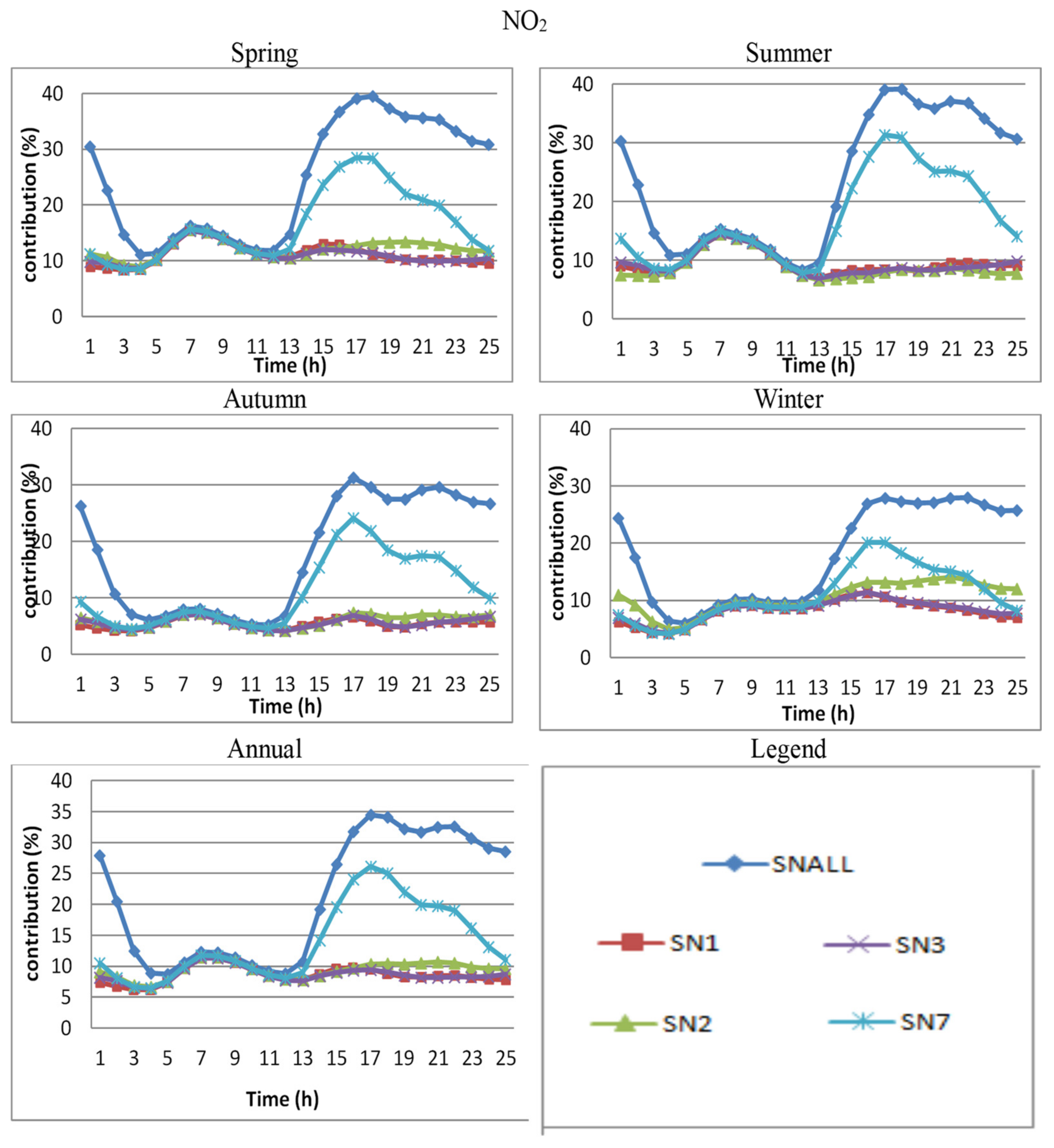
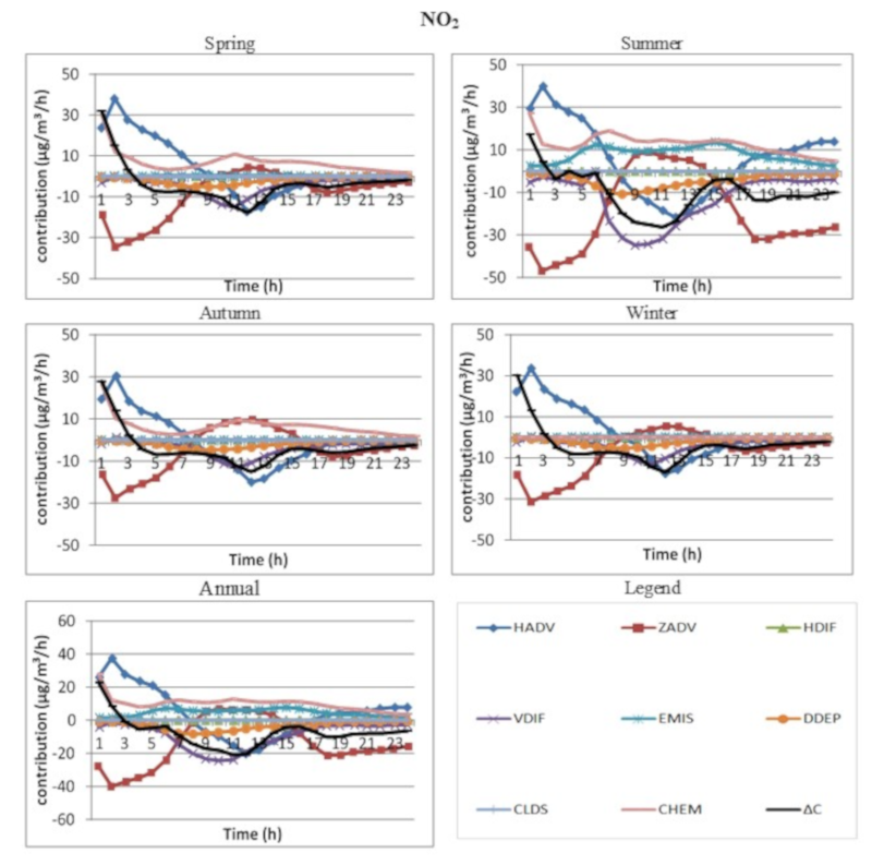
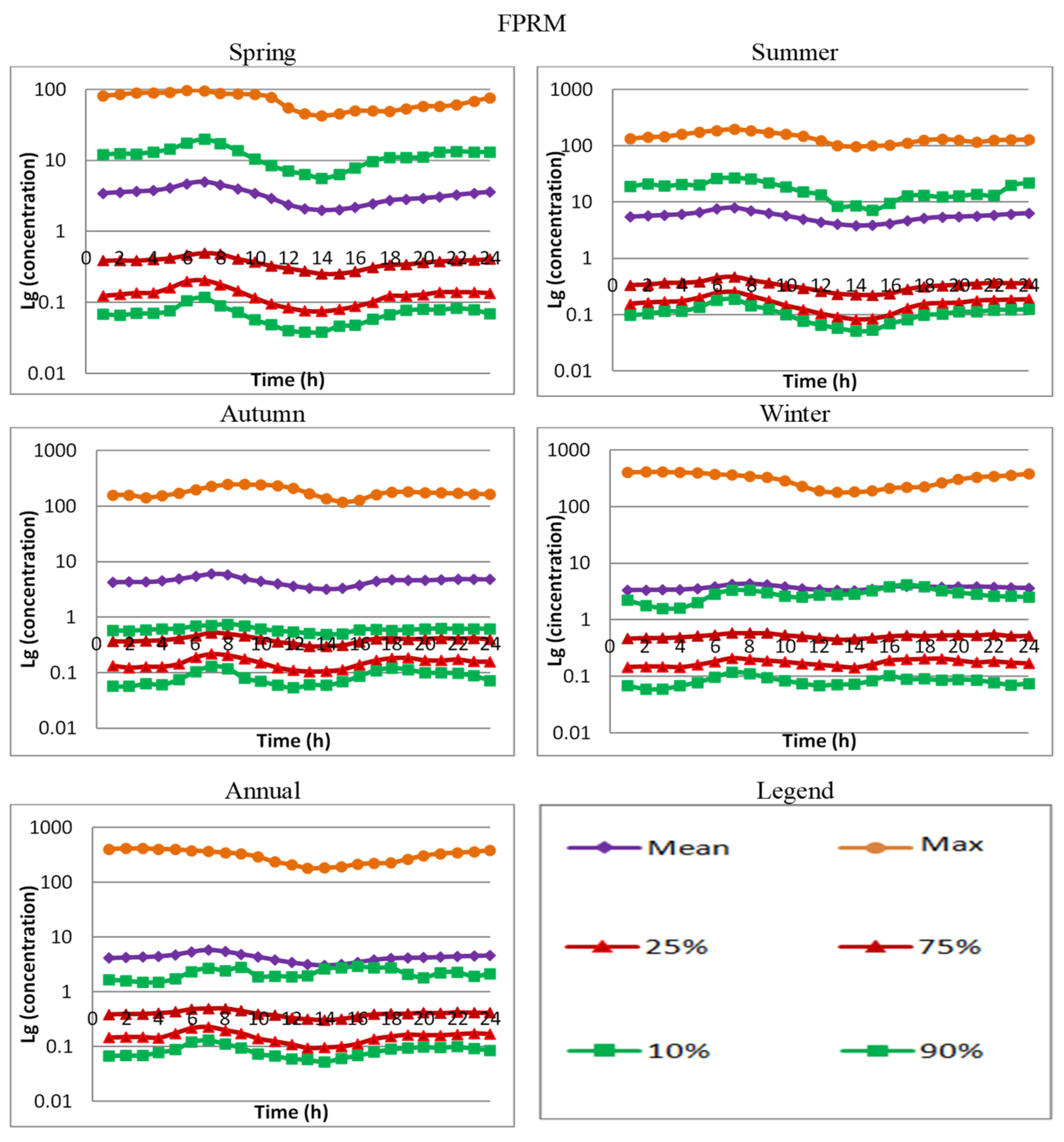
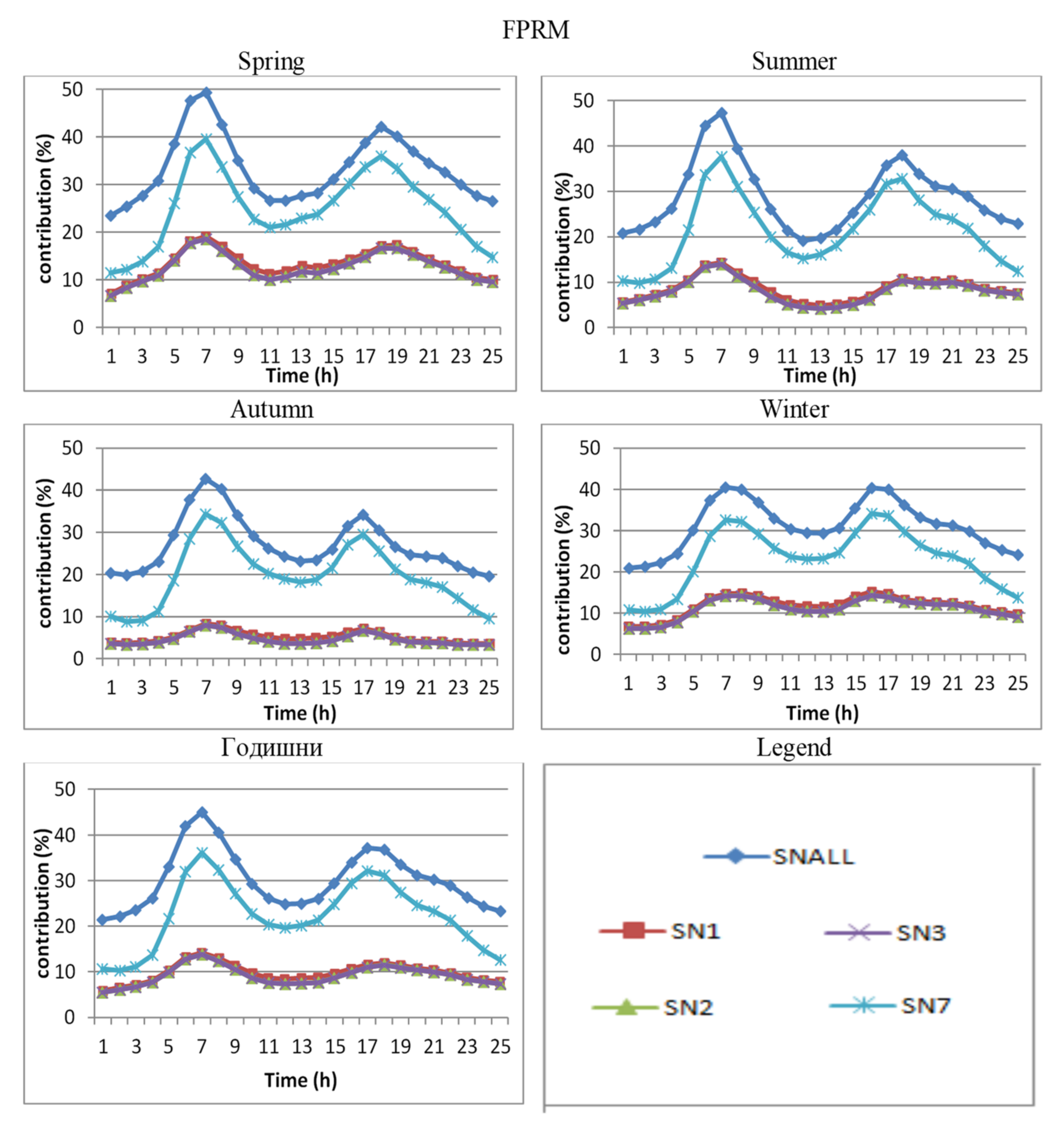
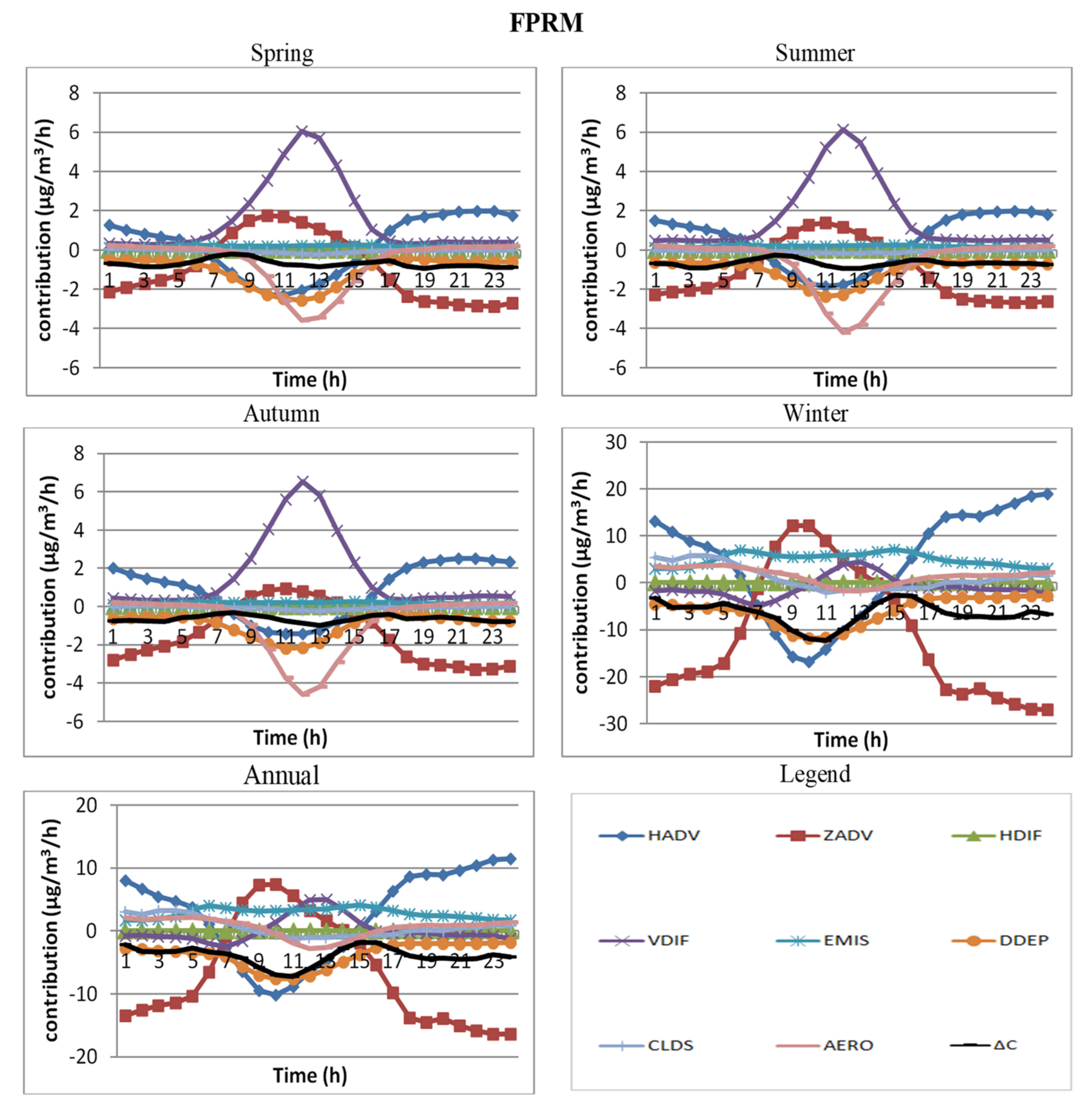
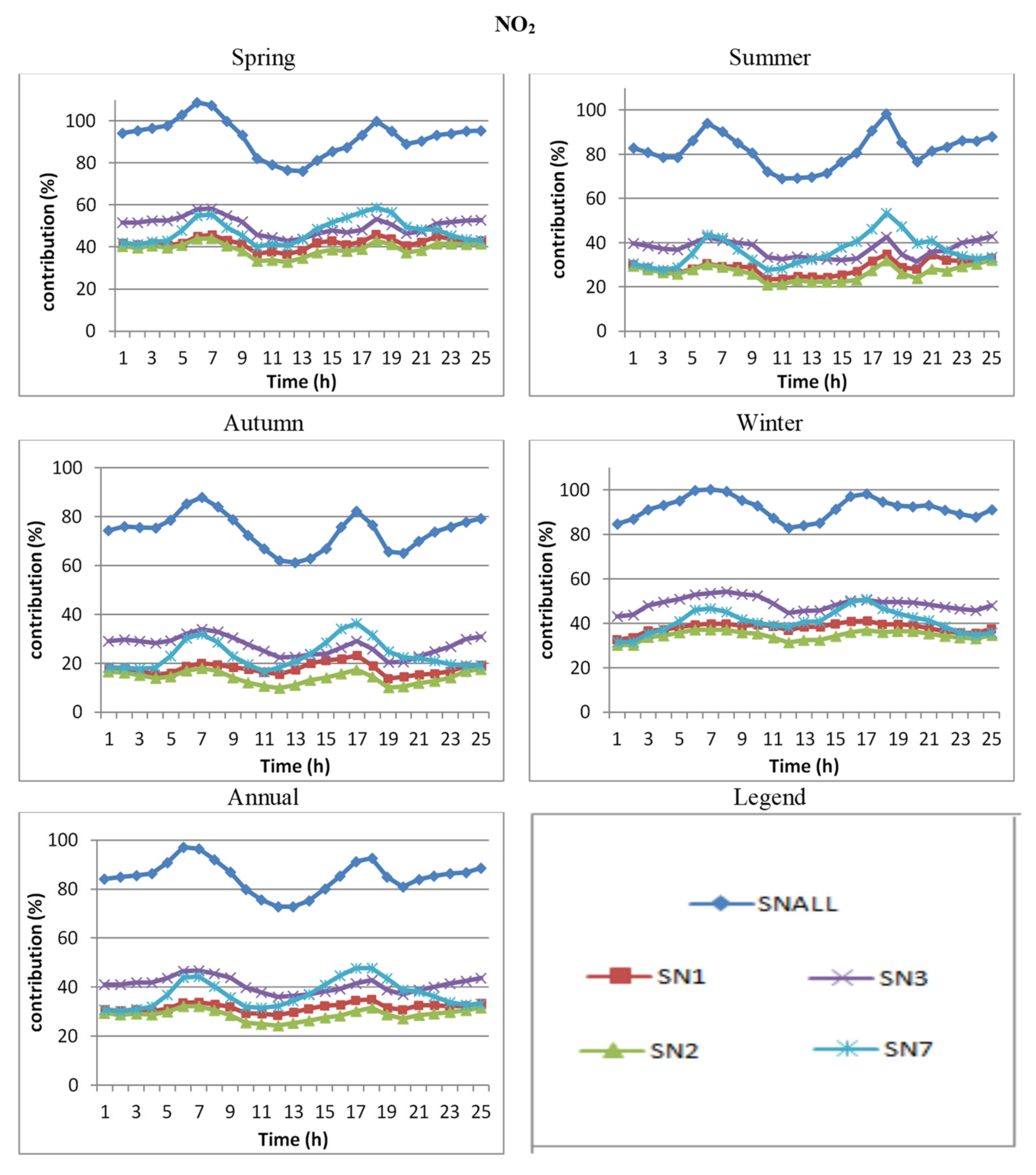
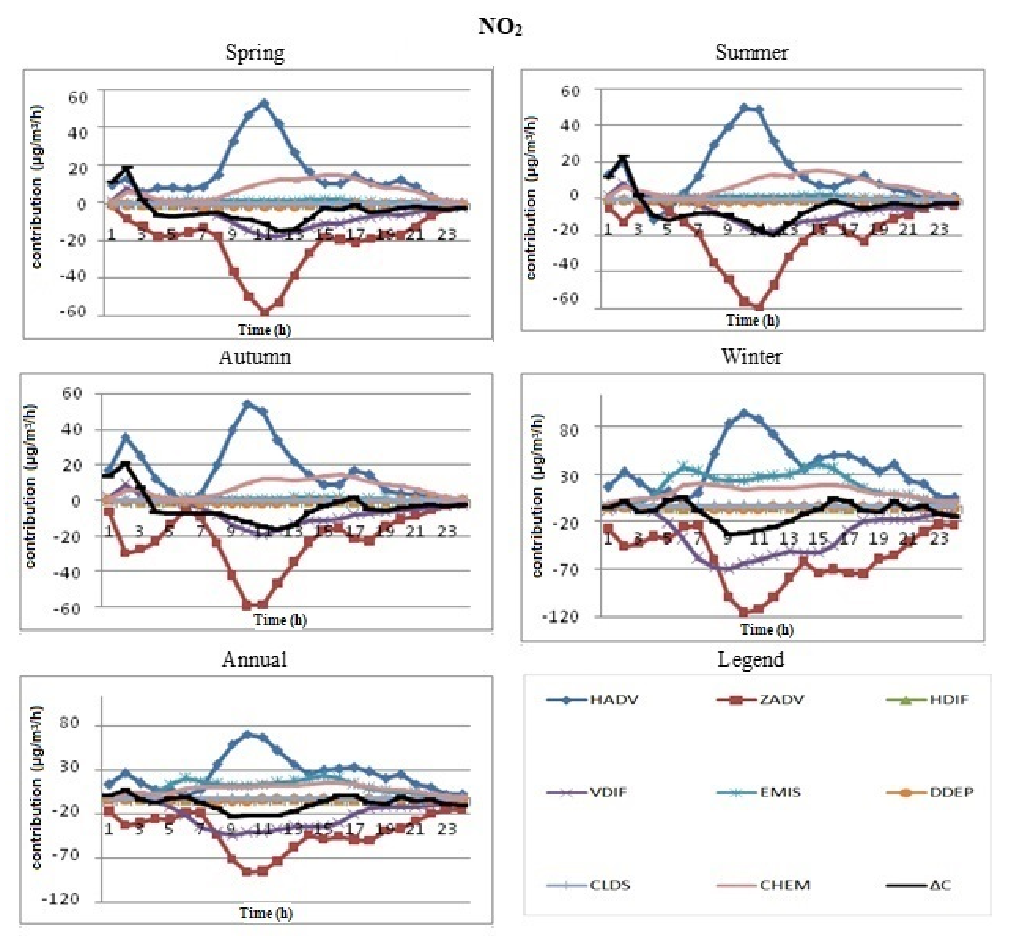
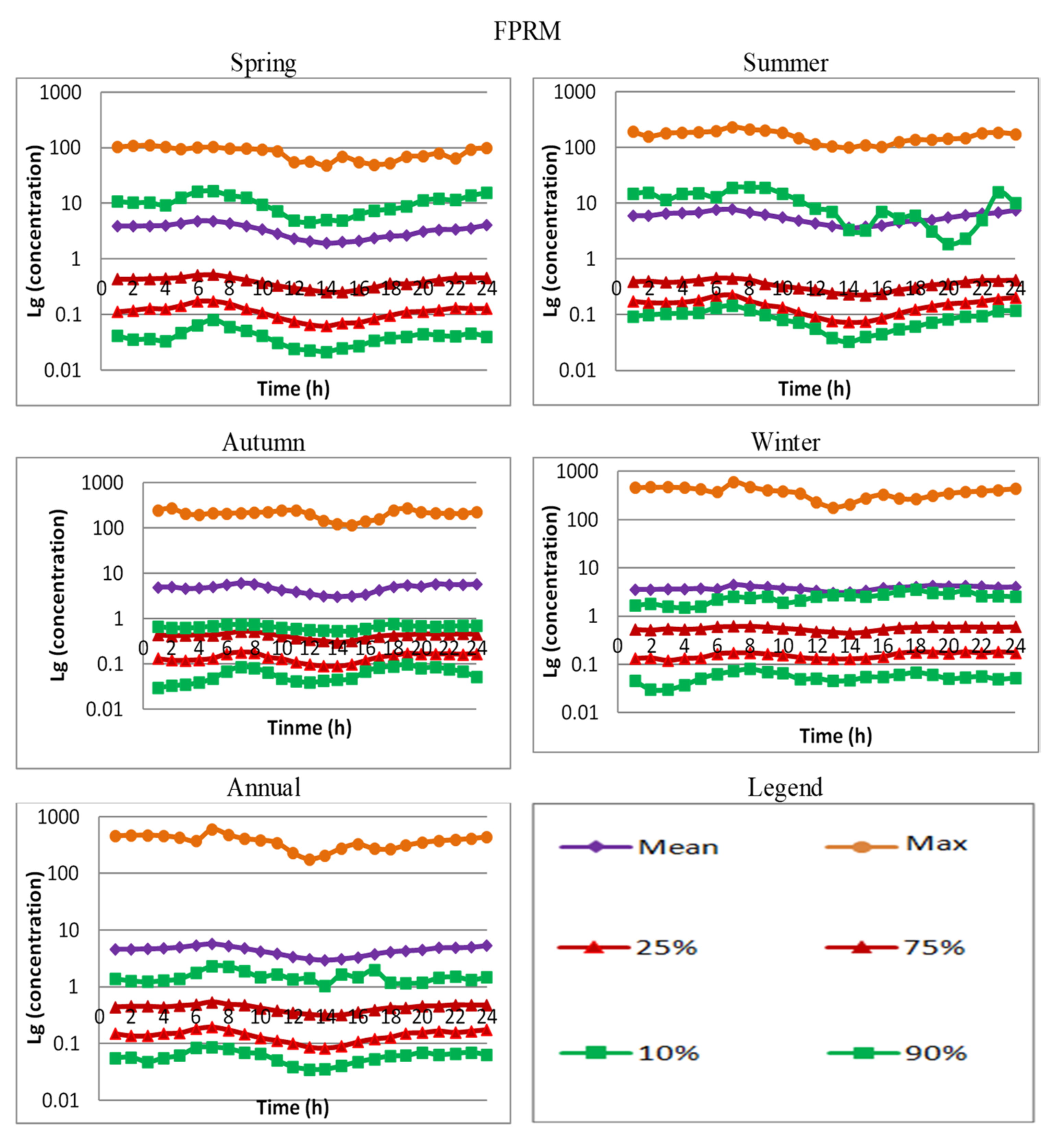
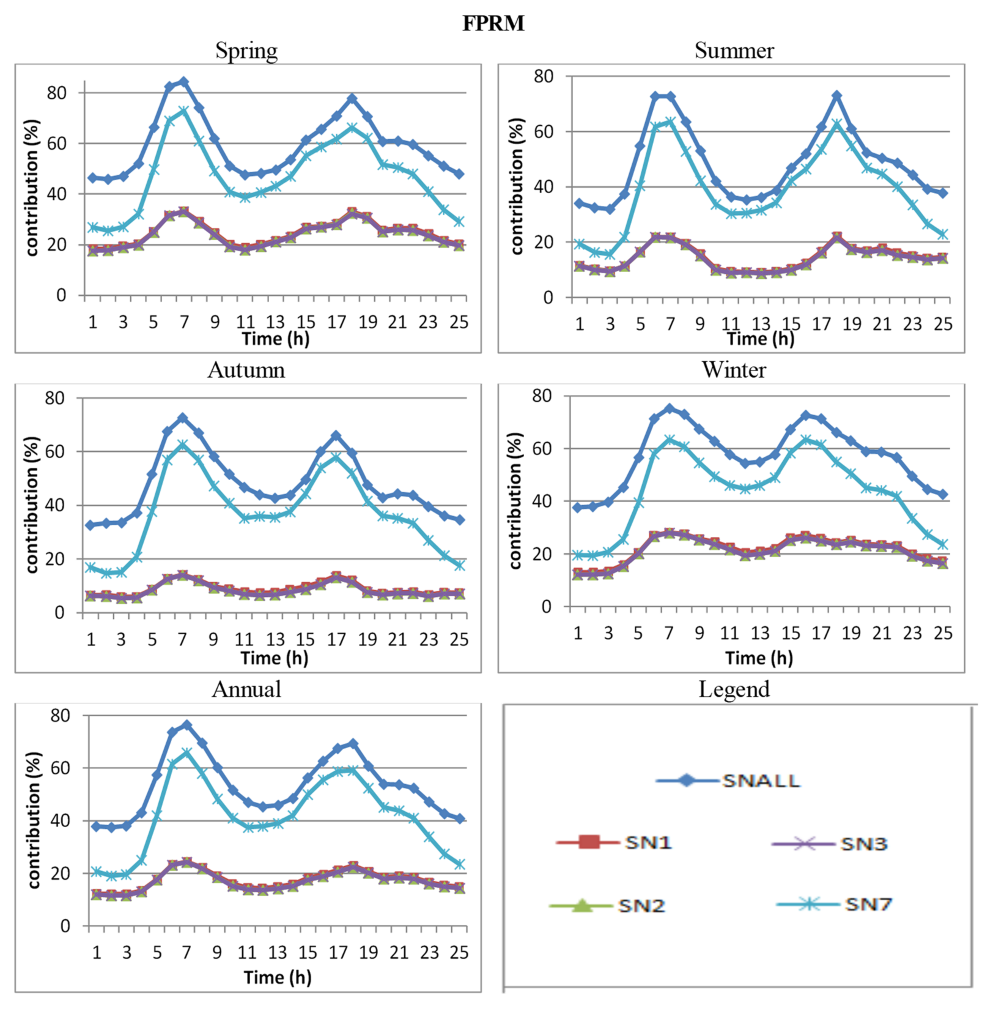
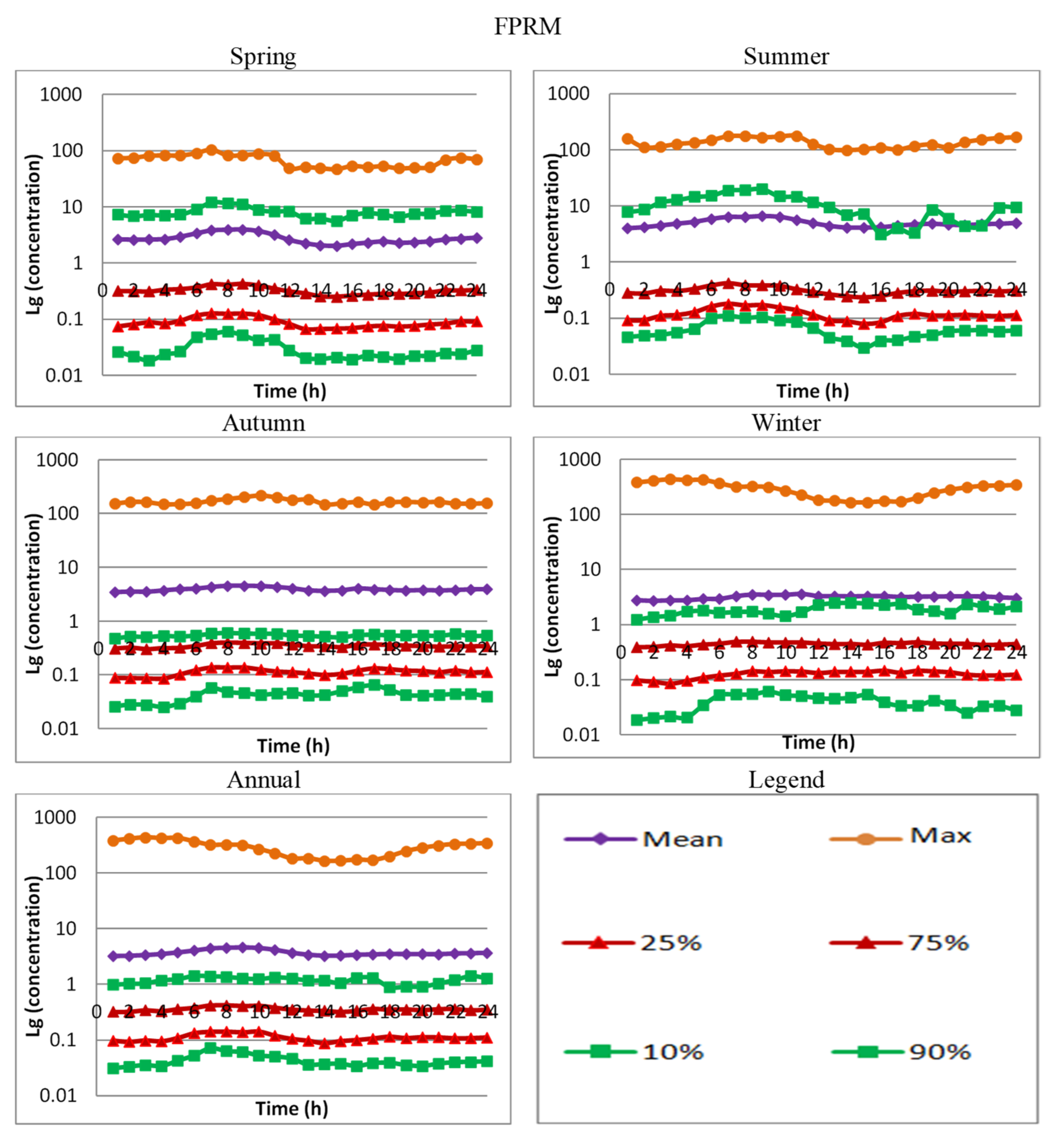
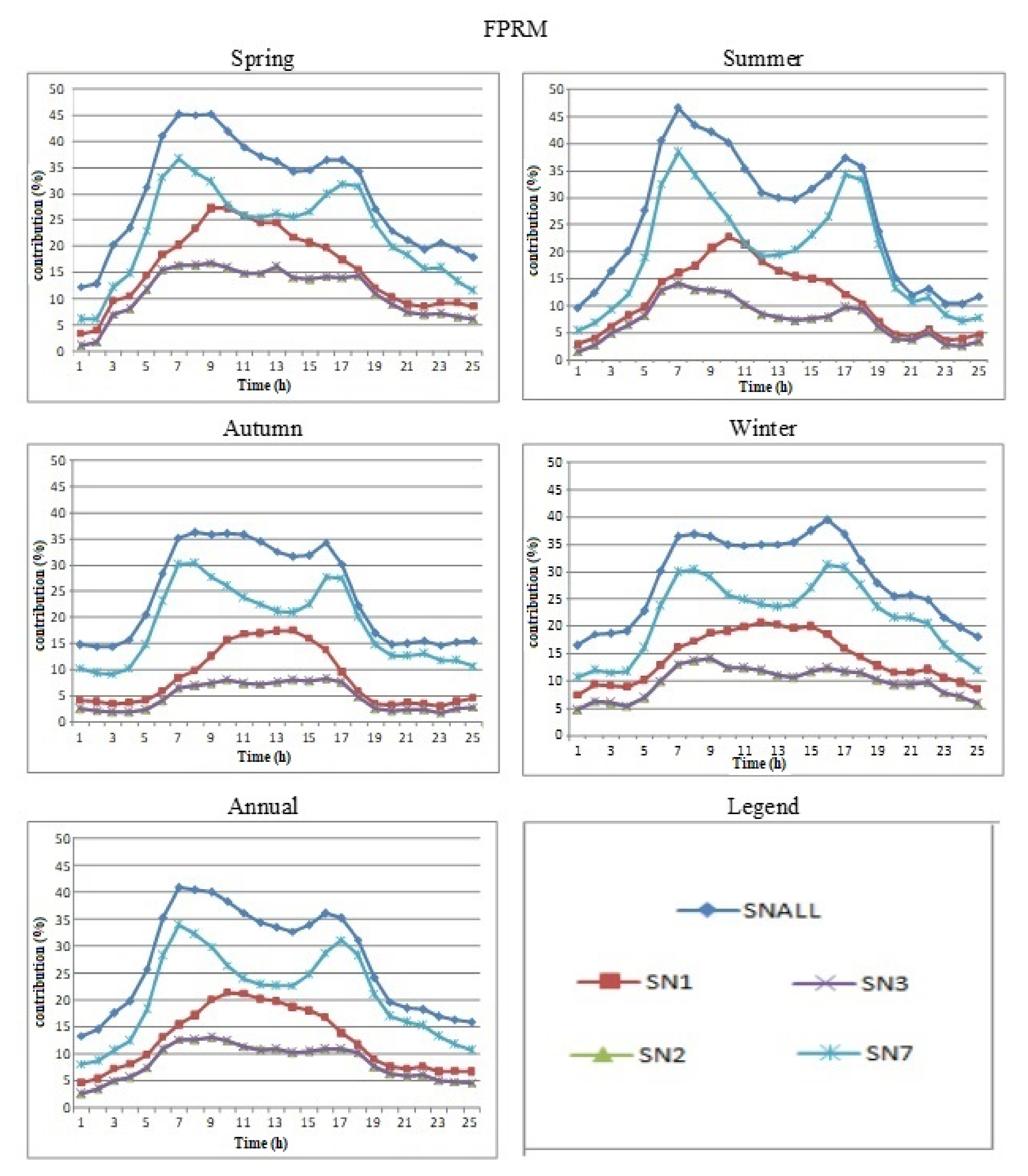
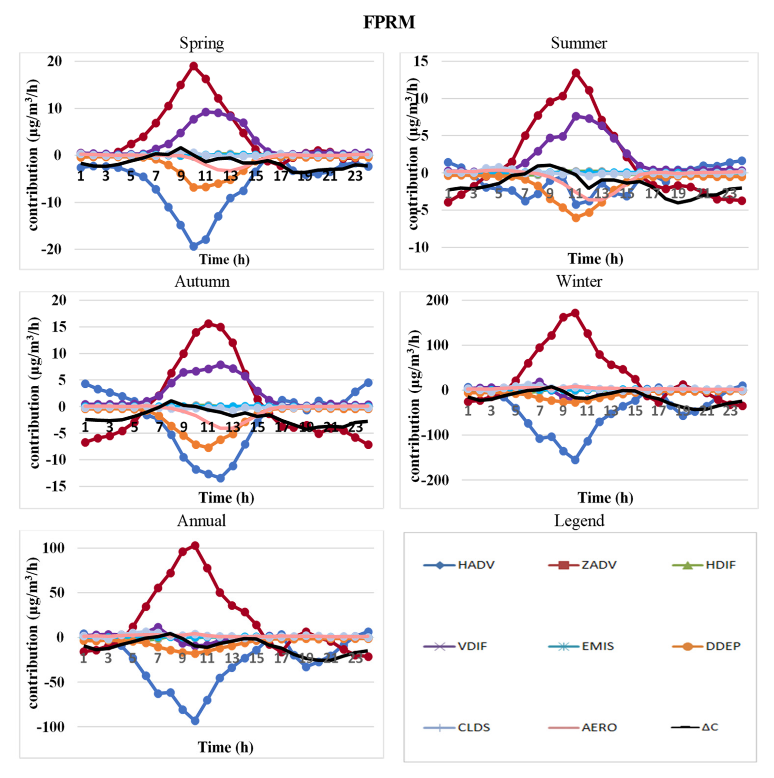
3.1. Characteristics of the Numerically Obtained Concentration Fields, Contribution of Different Emission Sources and Different Dynamic and Chemical Processes to the Atmospheric Composition in Sofia

The graphics in Figure 2 show that the average NO2 concentrations have a well-expressed diurnal course with a maximum in the early hours and a minimum in the afternoon. The average concentrations are mostly in the 80% interval of cases (between the two green curves 10–90%). The average concentrations are asymmetrically located in the different pieces of a number of case intervals during the day as well as in the different seasons. The seasonal course shows that the absolute maximum of NO2 concentrations are highest in the autumn and the winter, which is probably due to the bigger frequency of the stable atmospheric stratification cases and the impeded vertical turbulent transport of NO2. The averaged ensemble annual and seasonal contributions of the different sources (Figure 3), leading to the formation of surface NO2 in Sofia, sheds light from another perspective. The results suggest that the contribution of the different sources varies in each season but with a similar diurnal course. Everywhere during the night, the biggest natural contribution is from emissions of all SNAP categories, followed by one of the road transport (SNALL and SN7), about 30% around midnight during all seasons. The contribution of the other sources in the morning hours has a small peak of around 10%.
Figure 4 shows the annually and seasonally averaged contributions of the processes of NO2 formation averaged for the entire domain. The main contribution for the NO2 formation has chemical processes with a positive sign. The horizontal advection is positive in the morning and afternoon and becomes negative at noon. The vertical advection is opposite to the horizontal one. The dry deposition and vertical diffusion have a negative contribution, although with smaller magnitudes. We can outline the positive contribution of the emissions at all hours of the day. The contribution of the other processes is almost zero.
The plots in Figure 5 suggest that the average FPRM concentrations have a well-expressed diurnal and seasonal course and asymmetrical distribution during the day and seasons for different intervals. The average concentrations fall into the interval containing 80% of cases during the warm months and above that for the cold ones, as during the winter, coinciding with the 90% curve. The absolute maximum and average concentrations are highest in the autumn and winter (stable stratification). There is a well-expressed maximum during the early hours for NO2 and a minimum around noon. The possible reasons for that maximum are the stable atmosphere and intensive road traffic in the early morning. The results for the averaged by ensemble annual and seasonal contributions of any source leading to the formation of surface FPRM for Sofia city are different (Figure 6), suggesting that the contribution of the different sources varies seasonally but has an equal diurnal course. The dominating natural contribution is one of the sources of all SNAP categories (SNALL), about 40%, followed by one of the road transport (SN7), at about 30%. The contribution of the other sources is about 10% in all seasons. The diurnal distribution shows that the different SNAP categories have maximum contribution in the morning hours and afternoon, and minimum around noon and during the night, which correspond to the concentrations graphics.
The annually and seasonally averaged contributions of processes for FPRM formation averaged for the entire Sofia city domain are shown in Figure 7. The main positive contribution has vertical diffusion for the entire day and vertical advection around noon. The contribution of the vertical advection in the morning and afternoon is negative. The horizontal advection is opposite to the vertical one. The dry deposition has a negative contribution with a maximum around noon. The aerosol processes have a negative sign in all seasons except for winter. The processes are more active during the winter in comparison with other seasons. The winter is outlined with a large positive contribution of emissions and decreases to a negative contribution of vertical diffusion. The other processes have almost zero contributions.

3.2. Characteristics of the Numerically Obtained Concentration Fields, Contribution of Different Emission Sources and Different Dynamic and Chemical Processes to the Atmospheric Composition in Orlov Most

Figure 8 shows the annually and seasonally averaged NO2 concentrations for the Orlov most station. The results on the plots show that the average concentrations have a well-expressed diurnal course with a maximum in the early morning hours and a minimum in the afternoon. The average concentrations are mostly in the 80% interval of cases (between the two green curves, at 10–90%). The average concentrations are asymmetrically located in the different intervals of a number of cases during the day as well as the seasons. The seasonal course suggests that the absolute maximum NO2 concentrations are highest in autumn and winter. The last is probably due to the more cases with stable atmospheric stratification and the impeded turbulent exchange of NO2 in the vertical direction. The averaged contributions from the different sources for NO2 formation in each season are different but with an equal diurnal course (Figure 9). The main contribution during the night is from the emissions of all SNAP sources (SNALL)—about 80%, followed by traffic (SN7)—about 50%, in spring, summer, and autumn. The second largest contribution in winter is from the industry (SN3). The contribution of all other sources in the morning hours has a peak of about 20%. The contribution of the sources from non-industrial burning (SN2) is the least.
The average annual and seasonal contributions of the processes of NO2 for Orlov most are shown in Figure 10. The main contribution for NO2 formation is chemical processes, which have a positive sign, as well as a high positive contribution of emissions in winter. Horizontal advection is positive during the entire day, and vertical advection is opposite. Vertical diffusion also has a negative contribution, although with smaller values and a maximum around noon. The contribution of the other processes is at almost zero magnitude.
The annually and seasonally averaged concentrations of the FPRM for the Orlov most station are shown in Figure 11. The curves show that the average concentrations have well-expressed diurnal and seasonal courses and asymmetric location in different intervals of numbers of cases during the day and seasons. The average concentrations fall into the 80% cases interval during the warm months and the above interval for the cold months. The winter average concentrations coincide with the 90% curve. The absolute maximum and average concentrations are highest for autumn and winter (stable stratification). The early morning hours are characterized by well-expressed maximum and minimum around noon. Probable reasons for this maximum are the stable atmosphere and intensive traffic early morning, which probably play a role in the results for the ensemble annual and seasonal average contributions of different sources for the formation of FPRM (Figure 12). The contribution of the different types of sources varies among the seasons but with the same diurnal course. The main contribution is from sources of all SNAPs (SNALL)—about 70%—followed by the one of the road transport (SN7)—about 60%. The contribution from the other sources is about 20% in all seasons. The distribution during the course of the day has maximum contributions in the morning and afternoon and a minimum around noon and during the night.
Figure 13 shows the same characteristics as in Figure 10, but for the FPRM formation. The main positive contribution to the FPRM formation is vertical in the afternoon with vertical advection for all hours of the day. The phase of horizontal advection is opposite the vertical, which shows a negative contribution. The dry deposition is negative with a maximum around noon. The aerosol processes during all seasons except for winter have a negative contribution. The processes are more intense during the winter in comparison with the other seasons, which is outlined with a large positive contribution of emissions and which decreases to negative for vertical diffusion. The contribution of the other processes is almost zero.

3.3. Characteristics of the Numerically Obtained Concentration Fields, Contribution of Different Emission Sources and Different Dynamic and Chemical Processes to the Atmospheric Composition in Bistritsa

Figure 14 shows the annually and seasonally averaged NO2 concentrations for the Bistritsa station. The graphics show that the average concentrations have well-expressed diurnal course with a maximum in the early morning hours and a minimum in the afternoon. The average concentration curves follow the 75% and fall into the 80% interval of cases. The locations of the average concentrations are asymmetric for different pieces of the number of cases interval during the day and for the seasons. The seasonal course suggests that the maximum nitrogen dioxide concentrations are highest in autumn and winter. The ensemble-averaged contributions for surface NO2 formation at Bistritsa point (Figure 15) differ for each type of source and in each season, but their diurnal course is almost equal, although not for Orlov most. The contributions are positive, and the largest one in the afternoon and during the night is SNALL, followed by road transport (SN7). The contribution of the other sources in the morning hours peaks at about 20%. The contributions of the sources from energetics (SN1) and non-industrial burning (SN2) reach 15% in the afternoon during the spring and the winter.
The averaged annual and seasonal contributions of the processes of NO2 averaged for Bistritsa are shown in Figure 16. The main contribution for NO2 formation is chemical processes, which have a positive sign. Horizontal advection is positive in morning hours and negative at noon, with a peak for all seasons, and vertical advection is opposite. Vertical diffusion also has a negative contribution, although with smaller values and a maximum around noon. The contribution of the other processes is of almost zero magnitude.
The annually and seasonally averaged concentrations of the FPRM for the Bistritsa station are shown in Figure 17. The plots show that the average concentrations have a well-expressed diurnal and seasonal course and are asymmetrically located in different intervals of numbers of cases during the day and seasons. The average concentrations fall into the 80% cases interval during the warm months and above it for the cold months. The winter average concentrations coincide with the 90% curve. The absolute maximum and average concentrations are highest for autumn and winter. The early morning hours are characterized by a well-expressed maximum for NO2, with a minimum around noon, which may be due to the stable atmosphere and intensive traffic in the early morning, which probably influence the patterns of the contributions of different sources for surface FPRM formation around Bistritsa (Figure 18). The averaged contributions are different for each season. The main contribution is naturally from sources of all SNAP categories (SNALL)—about 40%—followed by road transport (SN7)—about 30%. In the afternoon, the sources from combustion in the production and transformation of energy (SN1) have a maximum of about 20%. The contribution from other sources is about 10% for all seasons. The daily distribution suggests that SNAPs have a maximum in the morning and afternoon and a minimum around noon and night.
Figure 19 shows the same characteristics as in Figure 16, but for FPRM formation. The main positive contribution to the FPRM formation is vertical diffusion for all hours of the day and vertical advection around noon. The phase of horizontal advection is opposite to the vertical one, which has a negative contribution. The dry deposition is negative with a maximum around noon. The processes are more intense during the winter in comparison with other seasons. The contribution of the other processes is almost zero.

4. Conclusions

Statistical processing was performed, and the probability density function was calculated for each of the atmospheric compounds with the corresponding seasonal and diurnal fluctuations for each of the points of the grid or the territory of the city. Two points were selected: a mountain type “Bistritsa” and a typical city “Orlov most.” Spatial and diurnal variations of the annual ensemble of NO2 and FPRM are considered. The minimum and maximum curves and the 25%, 75%, 10%, and 90% probability curves are shown. The curves show the imaginary concentrations for which the probability of each simulation is less than 25%, 75%, 10%, and 90%, respectively.
The concentrations of NO2, FPRM of Bistritsa are of the same order as Orlov Most. The NO2 and FPRM concentrations around noon are at a local minimum and are larger during morning hours due to the combination of factors, including traffic and atmospheric stability. The NO2 concentrations are at a minimum around noon, probably because of the more intense turbulent mixing and the slope effect. The FPRM concentrations do not have significant diurnal variations. The ensemble behavior of NO2 and FPRM is significantly asymmetric for both selected sites.
For all emission categories, the pattern of the contribution fields is complex, which reflects the emission source configuration and the heterogeneity of topography, land use, and meteorological conditions. Plots of this kind can give a good qualitative impression of the spatial complexity of emission contributions. In order to demonstrate emission contribution behavior in a simpler and easier way, the respective fields can be averaged over some domain, which makes it possible to follow and compare the diurnal behavior of the respective contributions of different species. The results presented in the paper are a first glance at the atmospheric composition status in urban areas; thus, few decisive conclusions can be made at this stage of the study. Different emissions, relative to contribution of the concentration of different species, can be different, varying from 80% to above 100%. The contributions of different emission categories to different species surface concentrations have different diurnal courses. For all of the pollutants, the contribution of SNALL is dominant, but this contribution of emissions is less than 100%, which means that part of the concentrations is formed from sources outside the Sofia city, due to transport into the domain. The contribution of all SN7 (road transport) to NO2 surface concentrations is positive and reaches about 50% around the busiest traffic roads. The SN7 emissions have dominant contributions to the NO2 and FPRM surface concentrations. The relative contribution of SNALL and SN7 to the formation of FPRM, as well as for NO2 at the busiest traffic place, have two maximums in the diurnal course.
The estimation of the contribution of emissions from different source categories is valuable information that can be useful for the definition of measures for improving the air quality in Sofia by reducing emissions. Moreover, knowing the diurnal course of the contributions for a specific time period can suggest an optimal emission temporal regime in order to mitigate air pollution for the given episode.
The results produced by the CMAQ “integrated process rate analysis” demonstrate the complex behavior and interaction of the different processes. Further analysis of these processes, their spatial, diurnal, and seasonal variability, and interaction can be helpful for an explanation of the overall picture and origin of the pollution in the considered region. For the entire domain of Sofia, and for each of the selected items, the total concentration change (ΔC), leading to a change in a concentration, is determined mainly by a small number of dominating processes that have large values and may have opposite signs and phases. The total concentration change (ΔC) is different for each pollutant. The sign of the contributions of some of the processes is obvious, but some may have different signs, depending on the type of emissions as well as weather conditions and topography. In general, it can be concluded that the contributions of different processes have different behaviors and interact in a complex way.
The “integrated process rate analysis” is not often applied in urban air quality simulations; thus, in the case of the present study, it enriches the entire picture of the atmospheric composition climate of the city of Sofia. This ensemble treatment of the contribution of different processes, however, does not give an easy answer to how the processes interact and how exactly they form the air composition. It will probably be more fruitful to consider the process contribution for a given episode together with the specific meteorological conditions for that episode.
The obtained results and the corresponding conclusions made in this paper are in good agreement with the general idea of how urban atmospheric composition is formed; thus, they do not add general knowledge on the subject. The research and applied contribution of the paper are that it presents quantitative estimations specific to the city of Sofia. Such an extensive and comprehensive study for the city of Sofia had not been made before.
The models and the entire procedure used in the present paper can, of course, be applied to other cities. Such studies have been made for many cities. A crucial point, however, is the emission inventory, and the activities for preparing it are specific for each city, depending on the raw data available.

Author Contributions

Conceptualization, I.G. and V.I.; methodology, I.G.; software, I.G.; validation, I.G. and V.I.; formal analysis, V.I.; investigation, V.I.; resources, I.G.; data curation, V.I.; writing—original draft preparation, V.I.; writing—review and editing, V.I. and I.G.; visualization, I.G.; supervision, V.I.; project administration, I.G.; funding acquisition, V.I. All authors have read and agreed to the published version of the manuscript.

Funding

This work has been carried out in the framework of the National Science Program “Environmental Protection and Reduction of Risks of Adverse Events and Natural Disasters”, approved by the Resolution of the Council of Ministers no. 577/17.08.2018 and supported by the Ministry of Education and Science (MES) of Bulgaria (agreement no. D01-363/17.12.2020) and has been partially supported by the National Center for High-performance and Distributed Computing (NCHDC), part of National Roadmap of RIs under grant no. D01-387/18.12.2020.

Institutional Review Board Statement

Not applicable.

Informed Consent Statement

Not applicable.

Data Availability Statement

The input data—large scale meteorological background and the emission inventories are described in the paper. The output from the computer simulations, which, after processing and generalization is the basis of the results, reported in the paper, is, unfortunately, still not publicly available. This is due to the requirements of the projects, which financially support the present study.

Acknowledgments

Deep gratitude to the organizations and institutes (TNO, NCEP/NCAR, ECA&D, Unidata, MPI-M and all others), which provide free of charge software and data. Without their innovative data services and tools, this study would not be possible.

Conflicts of Interest

The authors declare no conflict of interest.

References

  1. Syrakov, D.; Etropolska, I.; Prodanova, M.; Slavov, K.; Ganev, K.; Miloshev, N.; Ljubenov, T. Downscaling of Bulgarian Chemical Weather Forecast from Bulgaria Region to Sofia City, American Institute of Physics. Conf. Proc. 2013, 1561, 120–132. [Google Scholar]
  2. Dimitrova, R.; Velizarova, M. Assessment of the Contribution of Different Particulate Matter Sources on Pollution in Sofia City. Atmosphere 2021, 12, 423. [Google Scholar] [CrossRef]
  3. Georgieva, I.; Gadzhev, G.; Ganev, K.; Miloshev, N. Analysis of The Contribution of Different Processes (Chemical and Dynamical) Which form the Atmospheric Composition in Sofia. In Proceedings of the 19th International Conference on Harmonisation within Atmospheric Dispersion Modelling for Regulatory Purposes, Bruges, Belgium, 3–6 June 2019. [Google Scholar]
  4. Gadzhev, G.; Georgieva, I.; Ganev, K.; Miloshev, N. Contribution of Different Emission Sources to the Atmospheric Composition Formation in City of Sofia. Int. J. Environ. Pollut. 2018, 64, 47–57. [Google Scholar] [CrossRef]
  5. Gadzhev, G.; Georgieva, I.; Ganev, K.; Ivanov, V.; Miloshev, N.; Chervenkov, H.; Syrakov, D. Climate Applications in a Virtual Research Environment Platform. Scalable Comput. Pract. Exp. 2018, 19, 107–118. [Google Scholar] [CrossRef] [Green Version]
  6. Gadzhev, G.; Ganev, K.; Mukhtarov, P. HPC Simulations of the Atmospheric Composition Bulgaria’s Climate (on the Example of Coarse Particulate Matter Pollution). In Proceedings of the International Conference on High Performance Computing, Borovets, Bulgaria, 2–6 September 2019; Studies in Computational Intelligence; Springer: Cham, Switzerland, 2021; pp. 221–233. [Google Scholar]
  7. Gadzhev, G.; Ganev, K.; Mukhtarov, P. Statistical Moments of the Vertical Distribution of Air Pollution Over Bulgaria. In Proceedings of the 12th International Conference on Large-Scale Scientific Computing, Sozopol, Bulgaria, 10–14 June 2019; Lirkov, I., Margenov, S., Eds.; Lecture Notes in Computer Science (including subseries Lecture Notes in Artificial Intelligence and Lecture Notes in Bioinformatics); Springer: Cham, Switzerland, 2020; pp. 213–219. [Google Scholar]
  8. Gadzhev, G.; Ganev, K. Vertical Structure of Some Pollutant Over Bulgaria-Ozone and Nitrogen Dioxide. SGEM 2018, 18, 449–454. [Google Scholar] [CrossRef]
  9. Gadzhev, G.; Ganev, K.; Miloshev, N. Numerical Study of the Atmospheric Composition Climate of Bulgaria-Validation of the Computer Simulation Results. Int. J. Environ. Pollut. 2015, 57, 189–201. [Google Scholar] [CrossRef]
  10. Gadzhev, G.; Ganev, K.; Miloshev, N.; Syrakov, D.; Prodanova, M. HPC Simulations of the Fine Particulate Matter Climate of Bulgaria. In Proceedings of the 8th International Conference on Numerical Methods and Applications, Borovets, Bulgaria, 20–24 August 2014; Lecture Notes in Computer Science (Including Subseries Lecture Notes in Artificial Intelligence and Lecture Notes in Bioinformatics); Springer: Cham, Switzerland, 2015; pp. 178–186. [Google Scholar] [CrossRef]
  11. Gadzhev, G.; Ganev, K.; Miloshev, N.; Syrakov, D.; Prodanova, M. Analysis of the Processes Which form the Air Pollution Pattern over Bulgaria. In Proceedings of the 9th International Conference on Large-Scale Scientific Computations, Sozopol, Bulgaria, 3–7 June 2013; Lecture Notes in Computer Science (Including Subseries Lecture Notes in Artificial Intelligence and Lecture Notes in Bioinformatics); Springer: Berlin/Heidelberg, Germany, 2014; pp. 390–396. [Google Scholar] [CrossRef]
  12. Gadzhev, G.; Ganev, K.; Miloshev, N.; Syrakov, D.; Prodanova, M. Some Basic Facts about the Atmospheric Composition in Bulgaria-Grid Computing Simulations. In Proceeding of the 9th International Conference on Large-Scale Scientific Computations, Sozopol, Bulgaria, 3–7 June 2013; Lecture Notes in Computer Science (Including Subseries Lecture Notes in Artificial Intelligence and Lecture Notes in Bioinformatics); Springer: Berlin/Heidelberg, Germany, 2014; pp. 484–490. [Google Scholar] [CrossRef]
  13. Gadzhev, G.; Ganev, K.; Prodanova, M.; Syrakov, D.; Atanasov, E.; Miloshev, N. Multi-Scale Atmospheric Composition Modelling for Bulgaria. In Air Pollution Modeling and Its Application XXII; NATO Science for Peace and Security Series C: Environmental Security; Springer: Dordrecht, The Netherlands, 2013; Volume 137, pp. 381–385. [Google Scholar]
  14. Gadzhev, G.; Ganev, K.; Prodanova, M.; Syrakov, D.E.; Miloshev, N.; Georgiev, G. Some Numerically Studies of the Atmospheric Composition Climate of Bulgaria. In Proceeding of the AIP Conference Proceedings, Proceedings of the 5th International Conference for Promoting the Application of Mathematics in Technical and Natural Sciences, Albena, Bulgaria, 24–29 June 2013; pp. 100–111. [Google Scholar] [CrossRef]
  15. Brandiyska, A.; Ganev, K.; Syrakov, D.; Prodanova, M.; Miloshev, N.; Gadzhev, G. Bulgarian Emergency Response System for Release of Hazardous Pollutants-Brief Description and Some Examples. Int. J. Environ. Pollut. 2012, 50, 3–11. [Google Scholar] [CrossRef]
  16. Gadzhev, G.; Ganev, K.; Syrakov, D.; Miloshev, N.; Prodanova, M. Contribution of Biogenic Emissions to the Atmospheric Composition of the Balkan Region and Bulgaria. Int. J. Environ. Pollut. 2012, 50, 130–139. [Google Scholar] [CrossRef]
  17. Gadzhev, G.; Syrakov, D.; Ganev, K.; Brandiyska, A.; Miloshev, N.; Georgiev, G.; Prodanova, M. Atmospheric Composition of the Balkan Region and Bulgaria. Study of the Contribution of Biogenic Emissions. In Proceeding of the AIP Conference Proceedings, Proceedings of the 3th International Conference on Application of Mathematics in Technical and Natural Sciences, Albena, Bulgaria, 20–25 June 2011; pp. 200–209. [Google Scholar]
  18. Todorova, A.; Gadzhev, G.; Jordanov, G.; Syrakov, D.; Ganev, K.; Miloshev, N.; Prodanova, M. Numerical Study of Some High PM10 Level Episodes. Int. J. Environ. Pollut. 2011, 46, 69–82. [Google Scholar] [CrossRef]
  19. Ganev, K.; Syrakov, D.; Todorova, A.; Gadzhev, G.; Miloshev, N.; Prodanova, M. Study of regional dilution and transformation processes of the air pollution from road transport. Int. J. Environ. Pollut. 2011, 44, 62–70. [Google Scholar] [CrossRef]
  20. Todorova, A.D.; Ganev, K.G.; Syrakov, D.E.; Prodanova, M.; Georgiev, G.J.; Miloshev, N.G.; Gadjhev, G.K. Bulgarian Emergency Response System for Release of Hazardous Pollutants-Design and First Tests. In Air Pollution Modeling and Its Application XXI; NATO Science for Peace and Security Series C: Environmental Security; Steyn, D., Trini Castelli, S., Eds.; Springer: Dordrecht, The Netherlands, 2011; pp. 263–268. [Google Scholar] [CrossRef]
  21. Gadzhev, G.; Jordanov, G.; Ganev, K.; Prodanova, M.; Syrakov, D.; Miloshev, N. Atmospheric Composition Studies for the Balkan Region. In Proceedings of the 7th International Conference on Numerical Methods and Applications, Borovets, Bulgaria, 20–24 August 2010; Lecture Notes in Computer Science (Including Subseries Lecture Notes in Artificial Intelligence and Lecture Notes in Bioinformatics); Springer: Berlin/Heidelberg, Germany, 2011; pp. 150–157. [Google Scholar]
  22. Gadzhev, G.; Ganev, K.; Jordanov, G.; Miloshev, N.; Todorova, A.; Syrakov, D.; Prodanova, M. Transport and Transformation of Air Pollution from Road and Ship Transport-Joint Analysis of Regional Scale Impacts and Interactions. In Proceedings of the International Conference on Transport, Atmosphere and Climate, Aachen, Germany, Maastricht, The Netherlands, 22–25 June 2009; pp. 33–37. [Google Scholar]
  23. Ganev, K.; Syrakov, D.; Gadzhev, G.; Prodanova, M.; Jordanov, G.; Miloshev, N.; Todorova, A. Joint Analysis of Regional Scale Transport and Transformation of Air Pollution from Road and Ship Transport. In Proceedings of the 7th International Conference on Large-Scale Scientific Computations, Sozopol, Bulgaria, 4–8 June 2009; Lecture Notes in Computer Science (Including Subseries Lecture Notes in Artificial Intelligence and Lecture Notes in Bioinformatics); Springer: Berlin/Heidelberg, Germany, 2010; pp. 180–187. [Google Scholar] [CrossRef]
  24. Todorova, A.; Gadzhev, G.; Jordanov, G.; Syrakov, D.; Ganev, K.; Miloshev, N.; Prodanova, M. Numerical Study of Some High PM10 Levels Episodes. In Proceedings of the 7th International Conference on Large-Scale Scientific Computations, Sozopol, Bulgaria, 4–8 June 2009; Lecture Notes in Computer Science (Including Subseries Lecture Notes in Artificial Intelligence and Lecture Notes in Bioinformatics); Springer: Berlin/Heidelberg, Germany, 2010; pp. 223–230. [Google Scholar] [CrossRef]
  25. Todorova, A.; Syrakov, D.; Gadjhev, G.; Georgiev, G.; Ganev, K.G.; Prodanova, M.; Miloshev, N.; Spiridonov, V.; Bogatchev, A.; Slavov, K. Grid Computing for Atmospheric Composition Studies in Bulgaria. Earth Sci. Inform. 2010, 3, 259–282. [Google Scholar] [CrossRef]
  26. San, J.R.; Pérez, J.L.; Gonzalez-Barras, R.M. The Use of LES CFD Urban Models and Mesoscale Air Quality Models for Urban Air Quality Simulations. In Proceedings of the 1st International Conference on Environmental Protection and Disaster Risks EnviroRISK 2020, Sofia, Bulgaria, 29–30 September 2020; Dobrinkova, N., Gadzhev, G., Eds.; Studies in Systems, Decision and Control; Springer: Cham, Switzerland, 2021; pp. 185–189. [Google Scholar] [CrossRef]
  27. Gryning, S.E.; Batchvarova, E. Advances in Urban Dispersion Modelling. In Advances in Air Pollution Modeling for Environmental Security; NATO Science Series (Series IV: Earth and Environmental, Series); Faragó, I., Georgiev, K., Havasi, Á., Eds.; Springer: Dordrecht, The Netherlands, 2005; Volume 54. [Google Scholar] [CrossRef]
  28. Karagiannidis, A.; Poupkou, A.; Giannaros, T.; Giannaros, C.; Melas, D.; Argiriou, A. The Air Quality of a Mediterranean Urban Environment Area and Its Relation to Major Meteorological Parameters. Water Air Soil Pollut. 2015, 226, 2239. [Google Scholar] [CrossRef]
  29. Zanis, P.; Katragkou, E.; Markakis, K.; Lysaridis, I.; Poupkou, A.; Melas, D.; Kanakidou, M.; Psiloglou, B.; Gerasopoulos, E.; Zerefos, C.; et al. Effects on Surface Atmospheric Photo-Oxidants over Greece during the Total Solar Eclipse Event of 29 March 2006. Atmos. Chem. Phys. 2007, 7, 6061–6073. [Google Scholar] [CrossRef] [Green Version]
  30. Poupkou, A.; Symeonidis, P.; Lisaridis, I.; Melas, D.; Ziomas, I.; Yay, O.D.; Balis, D. Effects of Anthropogenic Emission Sources on Maximum Ozone Concentrations over Greece. Atmos. Res. 2008, 89, 374–381. [Google Scholar] [CrossRef]
  31. Katragkou, E.; Zanis, P.; Tegoulias, I.; Melas, D.; Krüger, B.C.; Huszar, P.; Halenka, T.; Rauscher, S. Decadal Regional Air Quality Simulations over Europe in Present Climate: Near Surface Ozone Sensitivity to External Meteorological Forcing. Atmos. Chem. Phys. 2010, 9, 10675–10710. [Google Scholar] [CrossRef] [Green Version]
  32. Kanakidou, M.; Mihalopoulos, N.; Kindap, T.; Im, U.; Vrekoussis, M.; Gerasopoulos, E.; Dermitzaki, E.; Unal, A.; Kocak, M.; Markakis, K.; et al. Megacities as Hot Spots of Air Pollution in the East Mediterranean. Atmos. Environ. 2010, 45, 1223–1235. [Google Scholar] [CrossRef]
  33. Im, U.; Poupkou, A.; Incecik, S.; Markakis, K.; Kindap, T.; Unal, A.; Melas, D.; Yenigun, O.; Topcu, S.; Odman, M.T.; et al. The Impact of Anthropogenic and Biogenic Emissions on Surface Ozone Concentrations in Istanbul. Sci. Total Environ. 2011, 409, 1255–1265. [Google Scholar] [CrossRef] [PubMed]
  34. Juda-Rezler, K.; Reizer, M.; Huszar, P.; Krüger, B.C.; Zanis, P.; Syrakov, D.; Katragkou, E.; Trapp, W.; Melas, D.; Chervenkov, H.; et al. Modelling the effects of climate change on air quality over Central and Eastern Europe: Concept evaluation and projections. Clim. Res. 2012, 53, 179–203. [Google Scholar] [CrossRef] [Green Version]
  35. Marécal, V.; Peuch, V.-H.; Andersson, C.; Andersson, S.; Arteta, J.; Beekmann, M.; Benedictow, A.; Bergström, R.; Bessagnet, B.; Cansado, A.; et al. A Regional Air Quality Forecasting System over Europe: The MACC-II Daily Ensemble Production. Geosci. Model Dev. 2015, 8, 2777–2813. [Google Scholar] [CrossRef] [Green Version]
  36. Shamarock, W.C.; Klemp, J.B.; Dudhia, J.; Gill, D.O.; Barker, D.M.; Duda, M.G.; Huang, X.-y.; Wang, W.; Powers, J.G. A Description of the Advanced Research WRF Version 3. 2007. Available online: https://opensky.ucar.edu/islandora/object/technotes%3A500/datastream/PDF/view (accessed on 20 October 2021).
  37. Byun, D.; Young, J.; Gipson, G.; Godowitch, J.; Binkowski, F.S.; Roselle, S.; Benjey, B.; Pleim, J.; Ching, J.; Novak, J.; et al. Description of the Models-3 Community Multiscale Air Quality (CMAQ) Modeling System. In Proceedings of the 10th Joint Conference on the Applications of Air Pollution Meteorology with the A&WMA; Phoenix, AZ, USA, 11–16 January 1998, pp. 264–268. Available online: http://www.epa.gov/asmdnerl/models3/doc/science/science.html (accessed on 20 October 2021).
  38. Byun, D.; Ching, J. Science Algorithms of the EPA Models-3 Community Multiscale Air Quality (CMAQ) Modeling System. Available online: https://cfpub.epa.gov/si/si_public_record_report.cfm?dirEntryId=63400&Lab=NERL (accessed on 20 October 2021).
  39. SMOKE v3.5.1 User’s Manual; The University of North Carolina at Chapel Hill: Chapel Hill, NC, USA, 2013; Available online: https://www.cmascenter.org/smoke/documentation/3.5.1/manual_smokev351.pdf (accessed on 20 October 2021).
  40. Vestreng, V. Emission Data Reported to UNECE/EMEP: Evaluation of the Spatial Distribution of Emissions. Meteorological Synthesizing Centre-West; The Norwegian Meteorological Institute: Oslo, Norway, 2001; Research Note 56, EMEP/MSC-W Note 1. [Google Scholar]
  41. Visschedijk, A.J.H.; Zandveld, P.Y.J.; Denier van der Gon, H.A.C. A High Resolution Gridded European Emission Database for the EU Integrate Project GEMS. Available online: http://lap.physics.auth.gr/gems/docu/TNO%20Short%20Emissions%20Report.pdf (accessed on 20 October 2020).
  42. Denier van der Gon, H.; Visschedijk, A.; van de Brugh, H.; Droge, R. A High Resolution European Emission Data Base for the Year 2005; TNO-Report TNO-034-UT-2010-01895 RPT-ML; Environment, Health and Safety: Utrecht, The Netherlands, 2010. Available online: https://webdosya.csb.gov.tr/db/necen/editordosya/file/NEC/MACC_Training/TNO_PAREST.pdf (accessed on 20 October 2020).
Figure 1. Five computational domains (CMAQ domains are nested in WRF ones)—D1 81 × 81 km (Europe), D2 27 × 27 km (Balkan Peninsula), D3 9 × 9 km (Bulgaria), D4 3 × 3 km (Sofia municipality) and D5 1 × 1 km (Sofia city).
Atmosphere 12 01450 g001
Figure 2. Spatial and diurnal variations of the annual and seasonal ensembles of surface NO2 (μg/m3) concentration behavior in logarithmic scale for Sofia for the period 2008–2014.
Atmosphere 12 01450 g002
Figure 3. Annual and seasonal averaged relative contribution (%) of all emissions and emissions from different SNAP categories to the formation of NO2 concentration in Sofia for the period 2008–2014.
Atmosphere 12 01450 g003
Figure 4. Annual, seasonal and diurnal course of the contribution of the different dynamic and chemical processes of the formation of NO2 concentrations (μg/m3/h) averaged for the territory of Sofia for the period 2008–2014.
Atmosphere 12 01450 g004
Figure 5. Spatial and diurnal variations of the annual and seasonal ensembles of surface FPRM (μg/m3) concentrations behavior in logarithmic scale for Sofia for the period 2008–2014.
Atmosphere 12 01450 g005
Figure 6. Annual and seasonal averaged relative contribution (%) of all emissions and the emissions from different SNAP categories of the formation of FPRM concentrations for Sofia for the period 2008–2014.
Atmosphere 12 01450 g006
Figure 7. Annual, seasonal and diurnal course of the contribution of the different dynamic and chemical processes for the formation of FPRM concentrations (μg/m3/h) averaged for the territory of Sofia for the period 2008–2014.
Atmosphere 12 01450 g007
Figure 8. Spatial and diurnal variations of the annual and seasonal ensembles of surface NO2 (μg/m3) concentrations behavior in logarithmic scale for Orlov most for the period 2008–2014.
Atmosphere 12 01450 g008
Figure 9. Annual and Seasonal averaged relative contribution (%) of all emissions and the emissions from different SNAP categories of the formation of NO2 concentrations for Orlov most for the period 2008–2014.
Atmosphere 12 01450 g009
Figure 10. Annual, seasonal and diurnal course of the contribution of the different dynamic and chemical processes of the formation of NO2 concentrations (μg/m3/h) averaged for Orlov most for the period 2008–2014.
Atmosphere 12 01450 g010
Figure 11. Spatial and diurnal variations of the annual and seasonal ensembles of surface FPRM (μg/m3) concentrations behavior in logarithmic scale for Orlov most for the period 2008–2014.
Atmosphere 12 01450 g011
Figure 12. Annual and seasonal averaged relative contribution (%) of all emissions and the emissions from different SNAP categories of the formation of FPRM concentrations for Orlov most for the period 2008–2014.
Atmosphere 12 01450 g012
Figure 13. Annual, seasonal and diurnal course of the contribution of the different dynamic and chemical processes to the formation of FPRM concentrations (μg/m3/h) averaged for Orlov most for the period 2008–2014.
Atmosphere 12 01450 g013
Figure 14. Spatial and diurnal variations of the annual and seasonal ensembles of surface NO2 (μg/m3) concentrations behavior in logarithmic scale for Bistritsa for the period 2008–2014.
Atmosphere 12 01450 g014
Figure 15. Annual and seasonal averaged relative contribution (%) of all the emissions and the emissions from different SNAP categories of the formation of NO2 concentrations for Bistritsa for the period 2008–2014.
Atmosphere 12 01450 g015
Figure 16. Annual, seasonal and diurnal course of the contribution of the different dynamic and chemical processes of the formation of NO2 concentrations (μg/m3/h) averaged for Bistritsa for the period 2008–2014.
Atmosphere 12 01450 g016
Figure 17. Spatial and diurnal variations of the annual and seasonal ensembles of surface FPRM (μg/m3) concentrations behavior in logarithmic scale for Bistritsa for the period 2008–2014.
Atmosphere 12 01450 g017
Figure 18. Annual and seasonal averaged relative contribution (%) of all the emissions and the emissions from different SNAP categories of the formation of FPRM concentrations for Bistritsa for the period 2008–2014.
Atmosphere 12 01450 g018
Figure 19. Annual, seasonal and diurnal course of the contribution of the different dynamic and chemical processes of the formation of FPRM concentrations (μg/m3/h) averaged for Bistritsa for the period 2008–2014.
Atmosphere 12 01450 g019
Publisher’s Note: MDPI stays neutral with regard to jurisdictional claims in published maps and institutional affiliations.

