Spatiotemporal Variability of Drought and Its Multi-Scale Linkages with Climate Indices in the Huaihe River Basin, Central China and East China

Abstract

With the aggravation of the ocean–atmosphere cycle anomaly, understanding the potential teleconnections between climate indices and drought/flood conditions can help us know natural hazards more comprehensively to better cope with them. This study aims at exploring the spatiotemporal patterns of drought and its multi-scale relations with typical climate indices in the Huaihe River Basin. First, the spatial patterns were identified based on the seasonal Standardized Precipitation Index (SPI)-3 during 1956–2020 by means of the Empirical Orthogonal Function (EOF). The two leading sub-regions of spring and winter droughts were determined. Then, we extracted the periodicity of spring and winter SPI-3 series and the corresponding seasonal climate indices (Arctic Oscillation (AO), Bivariate El Niño–Southern Oscillation (ENSO)Timeseries (BEST), North Atlantic Oscillation (NAO), Niño3, and Southern Oscillation Index (SOI)) and the sunspot number by using the Continuous Wavelet Transform (CWT). We further explored the teleconnections between spring drought, winter drought, and climate indices and the sunspot number by using Cross Wavelet Transform (XWT) and Wavelet Coherence (WTC) analyses. The results show that there are in-phase multi-scale relations between spring/winter PC1 and AO, BEST, and Niño3, of which the climate indices lead spring PC1 by 1.5–2 years and the climate indices lag winter PC1 by 1.5–3 years. Anti-phase relations between spring PCs and SOI and the sunspot number were observed. NAO mainly affects the interdecadal variation in spring drought, while AO and Niño3 focus on the interannual variation. In addition, Niño3 and SOI are more related to the winter drought on interdecadal scales. Moreover, there is a positive correlation between the monthly average precipitation/temperature and Niño3 with a lag of 3 months. The results are beneficial for improving the accuracy of drought prediction, considering taking NAO, AO, and Niño3 as predictors for spring drought and Niño3 and SOI for winter drought. Hence, valuable information can be provided for the management of water resources as well as early drought warnings in the basin.

1. Introduction

The Intergovernmental Panel on Climate Change’s Sixth Assessment Report (IPCCAR6) shows that global climate change will be further aggravated in the coming decades, intensifying the water cycle and indicating that more extreme droughts will occur in many regions all over the world [1]. Drought is a kind of complex and dynamically accumulating meteorological disaster, with negative impacts on socioeconomic development and ecosystem sustainability. Nowadays, researchers pay more attention to the teleconnection of drought and atmospheric circulation [2,3,4,5,6]. It is of great significance to understand the potential linkages between climate indices and drought variability in order to make reasonable predictions or assumptions about future regional droughts.

In recent years, a lot of research has been conducted to detect the possible relation between large-scale climate phenomena and droughts or floods in specific geographical locations [2,5,7,8,9,10,11,12,13,14,15,16,17,18,19,20,21,22,23]. Wahiduzzaman concluded that major flood events over Bangladesh occurred during the monsoon period, and most of them occurred under the La Niña condition [24]. Sobral et al. detected the relation between the annual SPI index and the El Niño–Southern Oscillation (ENSO), and found that the events of El Niño and La Niña were not directly related to the variation in rainfall in any region of South Rio de Janeiro (SRJ) [25]. Chen et al. analyzed the relations between temperature, drought, El Niño, La Niña, and sunspots in North China, and concluded that El Niño events always occur with increased temperature and decreased rainfall, which is the opposite of La Niña events. Regarding sunspots, there are negative correlations with temperature and rainfall [11]. Jin et al. explored the relationship between the ENSO and summer and winter precipitation in eastern China. The results showed that the warm phase of the ENSO has a good correlation with increased winter precipitation in eastern China [3]. Zou et al. detected the response of extreme rainfall to sunspots, the ENSO, and the Pacific Interdecadal Oscillation (PDO) in the lower reaches of the Yangze River, and found that sunspots exhibit the strongest effect, while the effect of the PDO is the weakest [26]. Wang et al. took the Loess Plateau as the study region and found that the ENSO and Western Pacific pattern (WP) have a significant influence on SPI-6 and SPEI-6, while the Pacific North American (PNA) teleconnection pattern has been more sensitive to SPI-12 and SPEI-12 for the past 57 years [27]. Xu et al. concluded that the ENSO mainly affects the interannual variation in drought, while the PDO and Arctic Oscillation (AO) mainly affect the interdecadal and interannual variation in Lanzhou, Northwest China [28]. Liu et al. evaluated the effect of the ENSO and AO on the winter drought variability in Shaanxi, North China, and showed that there are inverse multi-scale linkages with the ENSO and positive linkages with the AO in most of the study area [4]. Different climate indices always represent different climate phenomena in specific regions worldwide, which have a diverse impact on different areas. It is thus necessary to explore the teleconnection of climate events and atmospheric circulation in a particular region.

The Huaihe River Basin, one of the areas in which droughts most frequently occur in China, is located in the north–south climate transition belt in China. In recent decades, droughts have happened frequently and severely in most parts of the river basin, resulting in water resource shortages, crop failures, socioeconomic losses, and adverse ecosystem consequences [29,30,31]. A considerable number of studies have been conducted on the topic of the drought evolution in the Huaihe River Basin. The existing studies mainly focus on three aspects, i.e., the adaptability of drought indicators, drought centers and drought evolution trends in the basin, and forecasting droughts with reanalysis products. To be specific, Wang et al. evaluated the revised Palmer Drought Severity Index (PDSI) in the Huaihe River Basin and verified its application in drought monitoring and early warning systems [13]. Lu et al. found that there is an increasing trend of drought intensity by using the China-Z growing season index and found that the drought coping ability was relatively poor in the Huang-Huai-Hai River Basin based on nine evaluation indexes [32]. Ji et al. employed the Regular vine Copula to establish the joint distribution of multi-dimensional variables and took the ENSO, ENSO Modoki, North Atlantic Oscillation (NAO), Indian Ocean Dipole (IOD), and AO as the predictors to improve the accuracy of drought-level transfer prediction [33]. In addition, taking SPI as the index, Yao et al. extracted the shift in the drought center in the Huaihe River Basin during 1962–2016 and found that the drought center mainly diffused from the center of the river basin to the surrounding areas [6]. Although much progress has been made in understanding and predicting the drought evolution in the Huaihe River Basin, there remain some limitations. As previous studies usually analyzed the spatial and temporal patterns of drought by detecting the drought center and its shifts, it is necessary to further explore the spatiotemporal patterns of the drought by sub-regions. In addition, there are few studies on the correlation between the spatiotemporal patterns of drought and the large-scale climatic phenomena. Analyzing the spatiotemporal patterns of drought by sub-regions and revealing its correlation with the large-scale climatic phenomena are of great value for drought prediction and water management in the Huaihe River Basin.

Therefore, the main objectives of this paper are: (i) to identify the spatial patterns of monthly SPI-1 and seasonal SPI-3 of the Huaihe River Basin during 1956–2020, which are characterized by sub-regions; (ii) to extract the periodical oscillation feature of spring SPI-3, winter SPI-3, and the corresponding seasonal climate indices on the basis of (i); (iii) to detect the possible locally phase-locked behavior between drought and climate indices and reveal their phase relations; and (iv) to discuss the potential relation between meteorology events and the ENSO phase position.

2. Materials and Methods

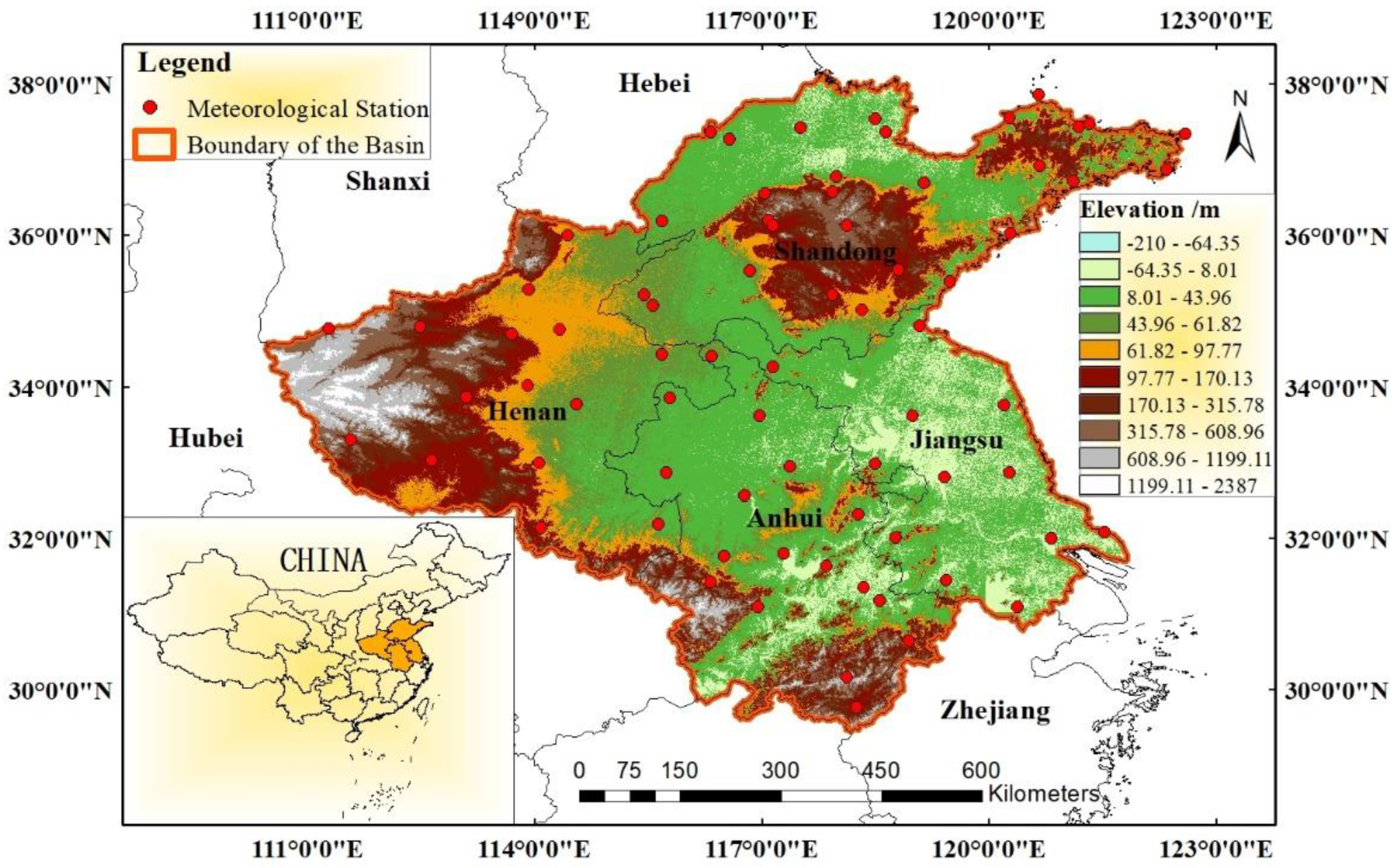
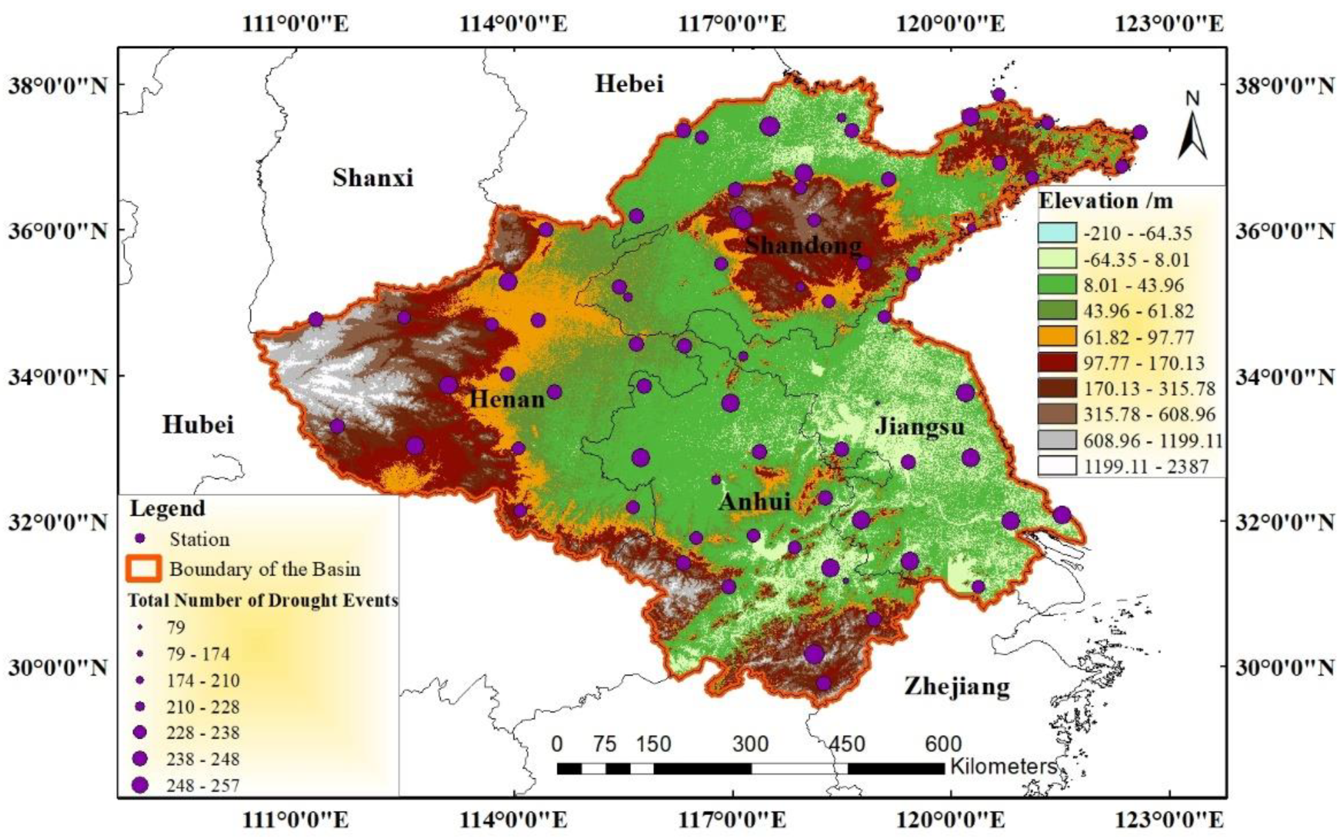
2.1. Study Area

The Huaihe River Basin is located in the north–south climate transition belt in China and borders the Yangtze River in the south and the Yellow River in the north. The basin stretches from 111°94′ E–121°25′ E and 30°95′ N–36°36′ N, with an area of 270,000 km². The west, southwest, and northeast of the basin are mountainous and hilly areas, while the rest are vast plains (Figure 1). The Huaihe River Basin is influenced by different climate features varying from north to south, i.e., a warm temperate semi-humid monsoon climate and a subtropical semi-humid monsoon climate. The basin is characterized by a hot and rainy summer and a cold and dry winter. In general, the temperature increases from north to south and from the coast to the inland, while the annual precipitation varies from south to north and from mountains to plains, which are greatly affected by the complex terrain. The annual average water surface evaporation is 900–1500 mm.

2.2. Data

The monthly precipitation values were obtained from the National Meteorological Information Center of China in order to calculate the standardized precipitation index (Section 2.3.1), which was applied to evaluate and define the drought severity. The website of the National Meteorological Information Center of China is http://data.cma.gov.cn/ (accessed on 16 May 2021). The 73 meteorological stations are spread across the basin as shown in Figure 1. The monthly precipitation values were quality-controlled in this study through two aspects. First, the meteorological data downloaded from the National Meteorological Information Center of China were subject to strict quality control and inspection, and the statistical results were manually checked by an extremum test and a time consistency test. Second, the default value of the precipitation data at all 73 stations in the Huaihe River Basin was replaced according to the meaning of the eigenvalue as explained in the data description document, i.e., 999,998 (without data) and 999,999 (lack of measurement) were replaced by the multi-year average of the corresponding month, and 999,990 (microscale) was replaced by zero. In addition, the start time of some data sequences lagged behind January 1956, indicating that there were gaps. The missing part (the gap) from January 1956 to the data sequence start time was supplemented by the ten-year moving average when the data start time lagged behind January 1956. There were 26 stations with gaps, accounting for 35% of the 73 stations, while the lag time of 18 stations was less than 5 years. The longest lag time was 20 years, i.e., the start time of the data sequence was January 1975, and occurred at only one station, while the second-longest lag time was 7 years. To summarize, 66 stations (accounting for 90% of the 73 stations) had more than 60 years of data.

Climate indices, i.e., the Niño3, AO, NAO, Bivariate ENSO time series (BEST), and Southern Oscillation Index (SOI), and sunspots were used to study the teleconnections with spring and winter droughts in the Huaihe River Basin. The climate index series, i.e., the monthly Niño3, AO, NAO, BEST, and SOI series, can be downloaded from the National Oceanic and Atmospheric Administration (NOAA) website (https://psl.noaa.gov/data/climateindices/list/, accessed on 7 July 2021). The monthly sunspot number can be obtained from the International Council for Science (ICSU)’s World Data System (WDS) (https://wwwbis.sidc.be/silso/home, accessed on 7 July 2021). Specifically, the Niño3 index, covering most of the area of the tropical Middle East Pacific Ocean (5 N–5 S,150 W–90 W), was used to represent the ENSO activity, which is a periodical atmosphere and ocean phenomenon with strong effects on global climate anomalies. The AO index represents the corresponding time coefficients of the first Empirical Orthogonal Function (EOF) of the monthly sea-level pressures north of 20° N, referring to the Arctic Oscillation. The NAO index is an effective indicator for assessing the North Atlantic Oscillation. The SOI index is the quantitative indicator of the Southern Oscillation, indicating the coherent interannual fluctuation in atmospheric pressure over the tropical Indo-Pacific region. BEST index series are calculated by combining a standardized SOI and a standardized Niño3.4 SST time series. The sunspot number is a measure of the daily solar activity, of which high values indicate intense activity and vice versa. The most direct effect of the sunspot number on the Earth is the magnetic field, which pushes the atmospheric circulation to longitudinal-direction flow, causing severe climate events. All the selected climate indices and the sunspot number have shown potential relations with meteorology events in China [8,34,35,36].

In this paper, the winter time series of climate indices and sunspots (hereinafter referred to as climate indices) refer to the corresponding values averaged for December, January, and February, and the spring time series were calculated by taking the average of March, April, and May.

2.3. Methodology

2.3.1. Standardized Precipitation Index (SPI)

The standardized precipitation index (SPI) is a drought evaluation index that represents the precipitation in a certain region within a given time using probability, which is applied to define the drought severity [37,38]. Positive and negative SPI values indicate wet and dry conditions, respectively, whose severity varies with magnitude. The SPI can be used to evaluate regional drought conditions above the monthly scale, e.g., 3 months for seasonal drought, 12 months for annual drought, 24 months and 36 months for multi-year drought, and so on [14,26,27]. It is a standardized index that makes comparisons possible and reliable in different regions.

The SPI is a satisfactory drought index for assessing the drought conditions in the Huaihe River Basin [29,39]. In this study, monthly SPI values, three-monthly SPI values, and twelve-monthly SPI values were calculated for a 65-year span (1956–2020) at 73 meteorological stations across the Huaihe River Basin (Figure 1). SPI-1 and SPI-12 were selected to assess the short-term and long-term water resource shortage conditions. SPI-3 was used to represent the seasonal drought for agriculture. The SPI-3 value of January was used to evaluate winter drought, the SPI-3 value of April was used to evaluate spring drought, the SPI-3 value of July was used to evaluate summer drought, and the SPI-3 value of October was used to evaluate autumn drought.

The first step in the SPI computation is the calculation of the probability density function of the precipitation within a given period, assuming a gamma or Pearson Type III distribution. Then, the probability density is standardized to a normal distribution. In the end, the drought severity is defined on the basis of the normalized cumulative frequency distribution.

$$f\left(x\right)=\frac{1}{{\beta }^{\gamma }\Gamma \left(x\right)}{x}^{\gamma -1}{e}^{\frac{-\gamma }{\beta }}\left(x>0\right)$$

(1)

where f(x) is the probability density function of precipitation series x, β is the scale parameter, and $\gamma$ is the shape parameter, both of which are greater than zero. The best performance β and $\gamma$ can be obtained by using a Maximum Likelihood Estimation.

$$\overline{\beta }=\raisebox{1ex}{$\overline{x}$}\!\left/ \!\raisebox{-1ex}{$\overline{\gamma }$}\right.$$

(2)

$$\overline{\gamma }=\frac{1+\sqrt{1+\raisebox{1ex}{$4A$}\!\left/ \!\raisebox{-1ex}{$3$}\right.}}{4A}$$

(3)

$$A=\log \overline{x}-\frac{1}{n}{\displaystyle \sum _{i=1}^n\log x_i}$$

(4)

where x_i is a sample in the precipitation series, $\overline{x}$ is the mean of the precipitation series, and n is the total number of samples in the precipitation series.

Then, for a specific precipitation x₀, the cumulative probability is:

$$P=F\left(x<x_0\right)={\displaystyle {\int }_0^{x_0}f(x)dx\begin{array}{cc}& \end{array}(x>0}).$$

(5)

When x is zero, the probability is:

$$P=F\left(x=0\right)=\frac{m}{n},$$

(6)

where m is the number of samples with zero precipitation, and n is the total number of samples in the precipitation series.

The normalized probability density with a gamma distribution is given by:

$$P=F\left(x<x_0\right)=\frac{1}{\sqrt{2\pi }}{\displaystyle {\int }_0^{x_0}{e}^{-\frac{z^2}{2}}}dx\begin{array}{cc}& \end{array}(x>0)$$

(7)

where z represents the SPI value.

The approximate solution of SPI (z) can be obtained by:

$$z=\mathrm{SPI}=\{\begin{array}{c}\frac{\left(c_{2}t+c_1\right)t-c_0-t}{\left[\left(d_{3}t+d_2\right)t+d_1\right]+1},P\le 0.5\\ \frac{-\left(c_{2}t+c_1\right)t+c_0+t}{\left[\left(d_{3}t+d_2\right)t+d_1\right]+1},P>0.5\end{array}$$

(8)

where $t=\sqrt{\ln \left(1/P^2\right)}$, c₀ = 2.515517, c₁ = 0.802853, c₂ = 0.10328, d₁ = 1.432788, d₂ = 0.189269, and d₃ = 0.001308 [40,41].

2.3.2. Empirical Orthogonal Function (EOF)

The Empirical Orthogonal Function (EOF), also known as Eigenvector Analysis or Principal Component Analysis, is a method for extracting the eigenvector of variables. It was first applied to climatology and meteorology by Lorenz in the 1950s and is now widely used to highlight potential physical mechanisms related to climate variability [6,16,17]. The spatial patterns (EOFs), the temporal series (PCs), and the eigenvalues are the outputs of the EOF analysis. The EOFs can identify the spatial modes of the variables by plotting them as vector maps, while the PCs represent the amplitude of each EOF mode over time. In addition, the modes are ranked by their significance to the overall variability according to the eigenvalues. In general, the leading modes can account for most of the original variability.

The computation steps are as follows.

Data preprocessing: process the selected data in the form of anomalies to obtain matrix $X_{m\times n}$.

$$C_{m\times n}=\frac{1}{n}X\times X^T$$

(9)

If $X_{m\times n}$ is anomalous, then $C_{m\times n}$ is a covariance matrix. If $X_{m\times n}$ is standardized, then $C_{m\times n}$ is a correlation coefficient matrix.

Eigenvalue matrix $E_{m\times m}$ and eigenvector matrix $V_{m\times m}$ must meet:

$$C_{m\times m}\times V_{m\times m}=V_{m\times m}\times E_{m\times m}$$

(10)

$$E_{m\times m}=\left[\begin{array}{cccc}{\lambda }_1& 0& \cdots & 0\\ 0& {\lambda }_2& \cdots & 0\\ \cdots & \cdots & \cdots & \cdots \\ 0& 0& \cdots & {\lambda }_m\end{array}\right]$$

(11)

where ${\lambda }_1>{\lambda }_2>\cdots >{\lambda }_m$. Each eigenvalue corresponds to a column eigenvector, i.e., an EOF.

$$P{C}_{m\times n}=V_{m\times m}^T\times X_{m\times n}$$

(12)

Each row of the PC represents the temporal series of the corresponding eigenvector.

The error in the eigenvector at the 95% confidence level is

$$\Delta \lambda =\lambda \sqrt{\frac{2}{N}}$$

(13)

where $\lambda$ is the eigenvalue and N is the degree of freedom (DOF) of the data. By means of detecting each $\lambda$ within the error range, if the neighbors overlap, the significance test has not been passed.

2.3.3. Continuous Wavelet Transform (CWT)

The continuous wavelet transform (CWT) is widely used in geographic physical studies as a time-series intermittent wave feature extraction tool that decomposes a signal into the time and frequency dimensions [42,43]. In all wavelet functions, the Morlet wavelet is widely used owing to its ability to balance the time and frequency performance, defined as

$${\psi }_0\left(\eta \right)={\pi }^{-1/4}{e}^{i{\omega }_0\eta }{e}^{-\frac{1}{2}{\eta }^2}$$

(14)

where ${\psi }_0$ is the wavelet generating function of the Morlet wavelet, ${\omega }_0$ is the dimensionless definite frequency, and $\eta$ is dimensionless time. The Morlet wavelet ${\omega }_0=6$.

The CWT of a time series ($x_n,n=1,\dots ,N$) is defined as:

$$W_n^X(s)=\sqrt{\frac{\delta t}{s}}{\displaystyle \sum _{n=1}^N{x}_n}{\psi }_0\left[(n^{\prime }-n)\frac{\delta t}{s}\right],$$

(15)

where $\delta t$ is the uniform time step, $s$ is the scale, and $\eta =s·t$. Usually, the wavelet power refers to ${\left|W_n^X(s)\right|}^2$.

Because the wavelet transform assumes that the data series is cyclic, the edge effect will appear in the wavelet power spectrum when the time series is of a finite length. Therefore, the Cone of Influence (COI) cannot be ignored, in which area the wavelet power caused by a discontinuity at the edge has dropped to $e^{-2}$ of the value at the edge.

The significant regions can be detected on the basis of the background spectrum and the desired confidence level. The null hypothesis is that the signal is generated by a stationary process with a given background power spectrum (P_k). Values other than the COI are estimated at a significance level of 5% at each scale. In general, the red noise spectrum is an appropriate background spectrum in studies on geophysical processes. The red noise was used and modeled as a lag-1 autoregressive (AR1) process.

$$P_k=\frac{1-{\alpha }^2}{{\left|1-\alpha e^{-2i\pi k}\right|}^2},$$

(16)

where k is the Fourier frequency index and $\alpha$ is the confidence level.

The probability that the wavelet power of the sequence with a given P_k is greater than p is

$$D\left(\frac{{\left|W_n^X\left(x\right)\right|}^2}{{\sigma }_X^2}<p\right)=\frac{1}{2}{P}_k{x}_v^2\left(p\right),$$

(17)

where v is 1 for a real wavelet and 2 for a complex wavelet.

2.3.4. Cross Wavelet Transform (XWT)

The cross wavelet transform (XWT) is a method used to expose regions with a high common power and further reveals information about the phase relationship (in-phase or anti-phase) and a consistent or slowly varying phase lag [9,42,44]. The XWT of the two time series $x_n$ and $y_n$ is defined as W^XY = W^XW^Y*, where * donates complex conjugation. |W^XY| is further defined as the cross-wavelet power.

Usually, the circular mean of the phase angles can be used to quantify the phase relationship plotted as arrows, in-phase pointing right and anti-phase pointing left. $x_n$ leads $y_n$ by pointing straight downward, while $x_n$ lags $y_n$ by pointing straight upward.

2.3.5. Wavelet Coherence (WTC)

The wavelet coherence can be used to reveal the coherence of the cross wavelet transform (XWT) in the time frequency space, i.e., to identify frequency bands and time intervals. Torrence and Webster defined the wavelet coherence of two time series as a function of the power spectrum density (PSD) and the cross-spectrum density (CSD) [43,44].

$$R_n^2\left(s\right)=\frac{{\left|S\left(s^{-1}{W}_n^{XY}\left(s\right)\right)\right|}^2}{S\left(s^{-1}{\left|W_n^X\left(s\right)\right|}^2\right)·S\left(s^{-1}{\left|W_n^Y\left(s\right)\right|}^2\right)},$$

(18)

where S is the smoothing operator, $W_n^X\left(s\right)$ and $W_n^Y\left(s\right)$ are the wavelet transforms of the two time series X and Y, respectively, and $W_n^{XY}\left(s\right)$ is the cross-wavelet spectrum of X and Y.

$$S\left(W\right)=S_{scale}\left(S_{time}\left(W_n\left(s\right)\right)\right),$$

(19)

where $S_{scale}$ denotes smoothing along the wavelet scale axis and $S_{time}$ denotes smoothing in time.

The statistical significance level of the wavelet coherence is estimated using Monte Carlo methods with red noise. Here, “coherence” usually means the squared WTC, ranging from 0 to 1, where 1 stands for the highest degree of coherence.

3. Results

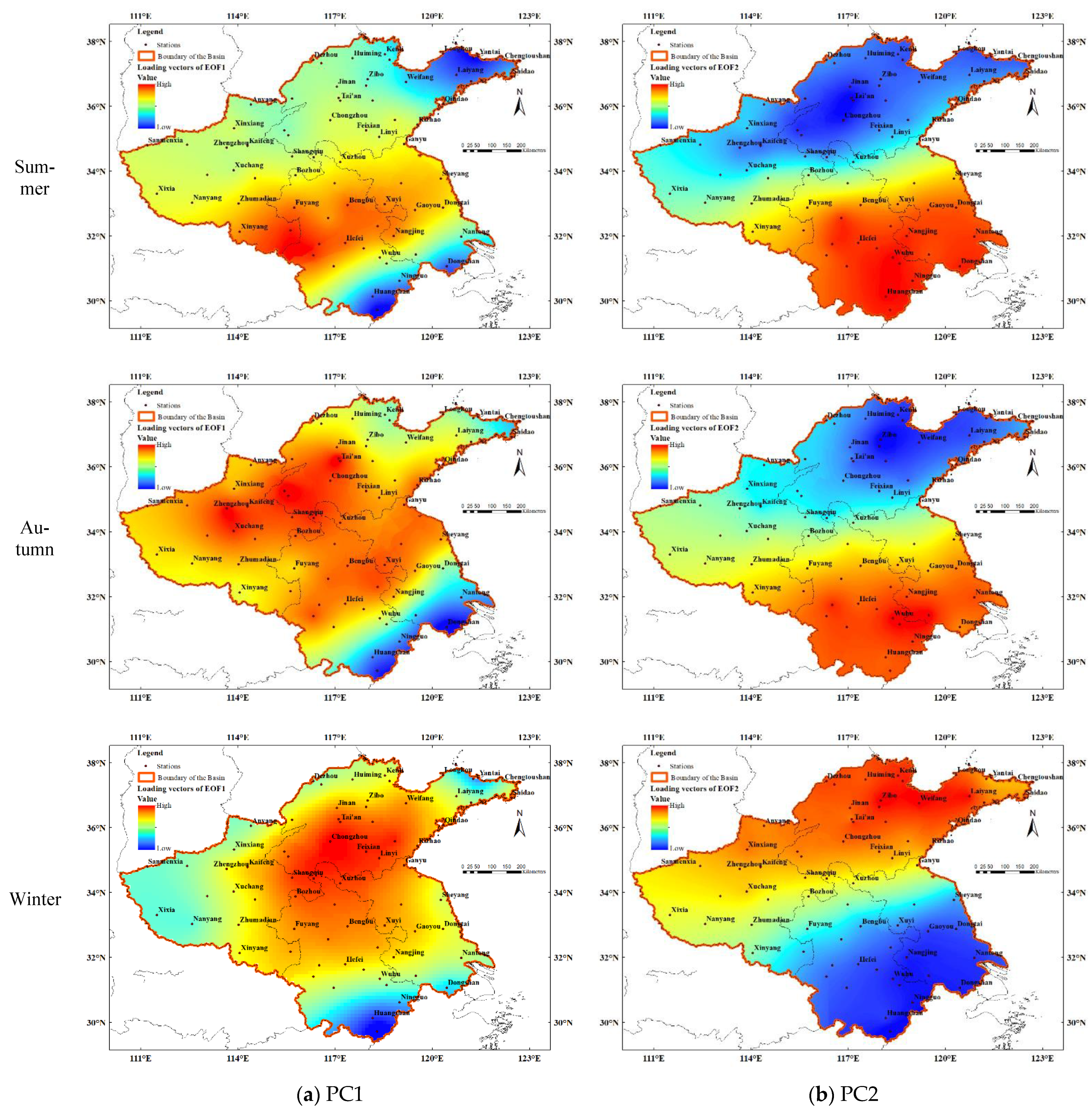
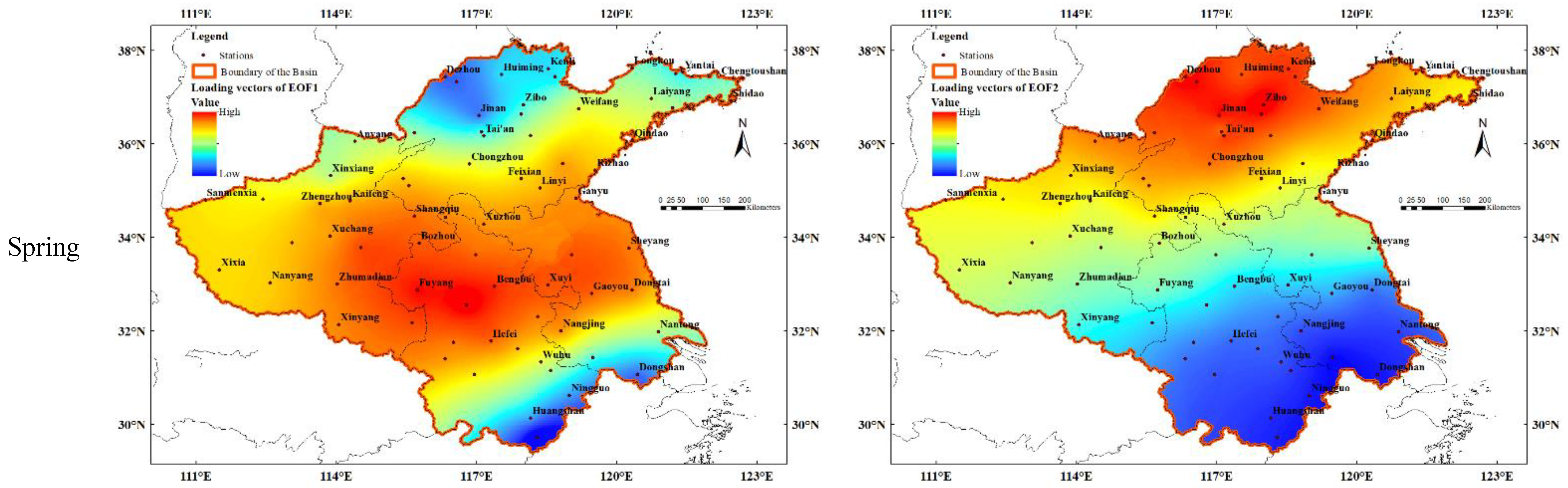
3.1. Spatiotemporal Variability in Drought Conditions

The spatial and temporal patterns of the seasonal (spring, summer, autumn, and winter) drought condition over the whole river basin were detected by conducting an EOF analysis based on the SPI-3 value series. The monthly drought condition was analyzed according to the SPI-1 value series. The eigenvalues of the leading EOFs are presented in

Table 1. The leading EOFs of seasonal SPI-3 and SPI-1 over the Huaihe River Basin.

Season	Mode	Percent Variance Explained (%)	Cumulative Variance (%)
Spring	PC1	60.44	60.44
	PC2	12.99	73.43
	PC3	4.53	77.96
Summer	PC1	32.46	32.46
	PC2	16.82	49.28
	PC3	9.16	58.43
Autumn	PC1	37.35	37.35
	PC2	17.32	54.67
	PC3	10.77	65.44
	PC4	4.61	70.05
Winter	PC1	59.80	59.80
	PC2	14.49	74.29
	PC3	7.27	81.57
	PC4	3.46	85.03
SPI-1	PC1	48.88	48.88
	PC2	14.43	63.31
	PC3	6.86	70.17
	PC4	3.93	74.10

, which all pass the significance test at the 95% confidence level. It is obvious that the first two EOFs of all seasons (except summer) and the SPI-1 series account for over 50% of the total variance, indicating that the complexity of the spatial pattern of the drought conditions over the river basin can largely be explained by the first two EOFs. Therefore, the spatial structure of the first two EOFs of all seasons and SPI-1 are presented in Figure 2 and Figure 3 to identify the corresponding spatial variability characteristics.

As shown in Figure 2, there is an area of strong spatial coherence characterized by the high loading vector values covering the middle part of the study area (almost all of the river basin) in the spatial distribution of EOF1 for all seasons. Although the core area is slightly different, the consistency of EOF1 proves that the drought is a kind of continuous natural disaster in both time and space. In addition, the distribution characteristics of EOF2 in spring and winter are similar to each other, indicating a sub-region with strong loading vector values in the northern part of the river basin. Additionally, there is a sub-region, i.e., the southern part of the river basin, in terms of the EOF2 modes in summer and autumn. The corresponding PC time series for the EOFs were analyzed to demonstrate the temporal variability in the drought conditions. Drier trends of winter and spring SPI-3 can be found for the northern part of the river basin (EOF2), while there are drier trends of spring and autumn for the middle part (EOF1) and indistinct wetter trends of winter for the middle part (EOF1). There are indistinct drier trends in summer and autumn for the southern part of the river basin (EOF2). The spatiotemporal characteristics of the EOF analysis in the SPI-1 value series are similar to those in spring and winter.

To summarize, the spatiotemporal variability in the Huaihe River Basin seems to be localized well, with three distinct sub-regions regarding various geographical and climatic variations. Considering that spring and winter droughts are more common, more changeable, and of a greater influence in the Huaihe River Basin, the climatic characteristics of winter and spring droughts will be further studied in this paper.

3.2. Periodicity of Spring SPI-3, Winter SPI-3, and Climate Indices

To identify the periodical oscillations of drought and climate indices, the CWT was conducted on eight time series for spring and winter, respectively, including two PCs of each season and the six corresponding seasonal climate indices, the results of which are shown in Figure 4. Obviously, the sunspot number in the time series fluctuates constantly in a 10–13-year band, which is consistent with the 11.2-year average activity circle as scholars have already shown. The SPI-3 spring time series of the EOF1 sub-region shows significant wavelet power in the 3.5–7-year band during 1992–2008 and in the 2–3-year band from 1965 to 1968. The power spectrum of the SPI-3 winter time series of EOF1, representing the middle part of the river basin, is distributed in a 2–4-year band from 1969 to 1976, during the periods of 1992–2001 and 2011–2015. Additionally, it can be observed that the wavelet power spectrum of winter PC1 closely resembles those of the BEST, Niño3, and SOI series, while the power spectrum of winter PC2 is consistent with that of the NAO and AO series. In addition, a few synchronous oscillation periods were found between spring PC1 and the NAO series as well as the SOI series, and the wavelet power spectrum of spring PC2 resembles those of BEST, AO, and Niño3.

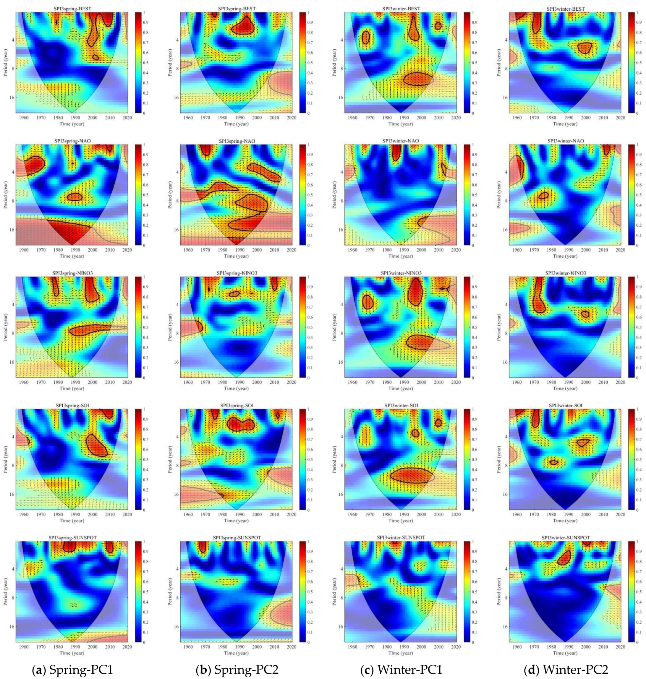
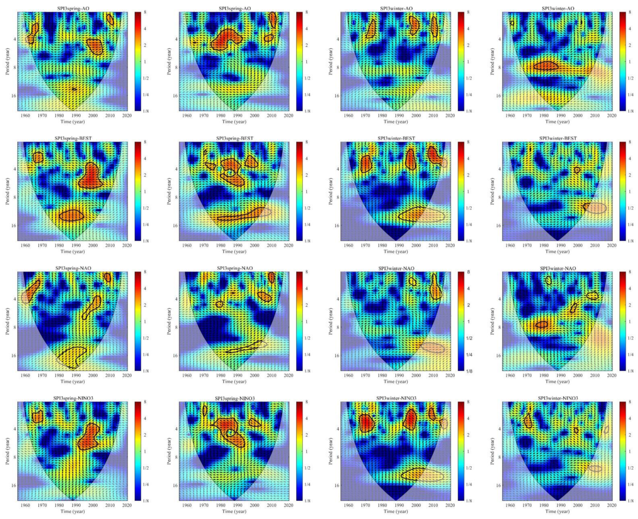
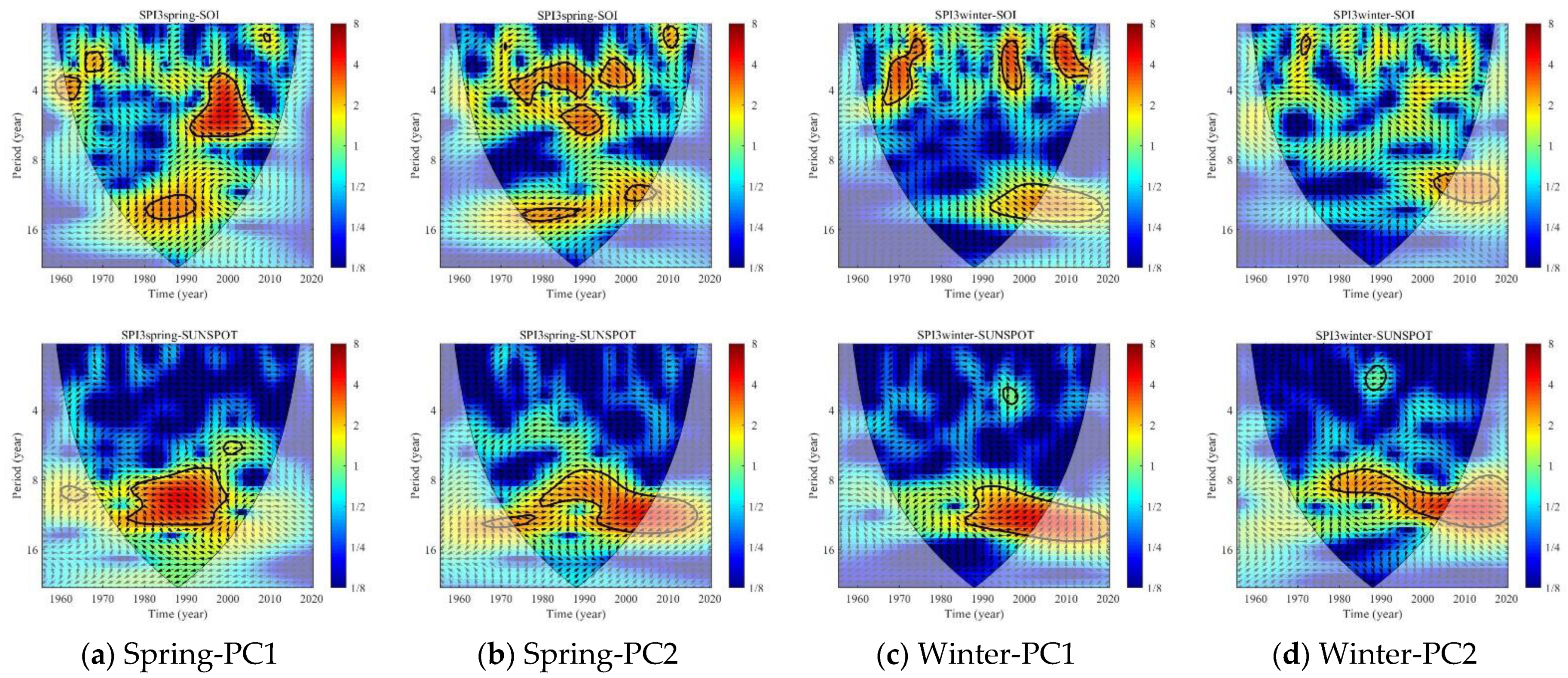
3.3. Multi-Scale Linkages between Spring SPI-3, Winter SPI-3, and Climate Indices

The WTC analysis was performed to further identify the possible multi-scale relationships and the locally phase-locked properties between the PCs of spring and winter and the corresponding climate indices. The EOF1 sub-region of spring and the AO have significant coherence around the 1–2-year band during 2002–2012 and an over 14-year band from 1980 to 2000 as illustrated in Figure 5a. Figure 5a also illustrates significant coherence with BEST around the 1–5-year band from 1996 to 2000 and the 1–2-year band during 2004–2011. The EOF1 sub-region of spring and the NAO have significant coherence around the 2–4.5-year, the 7–8-year, and the over 14-year bands for different time stages. Additionally, there are 1–3-year, 1–4-year, and 7–8-year bands with significant coherence in the wavelet coherence spectrum of spring EOF1 and Niño3. It is shown in Figure 5a that the significant coherence between spring EOF1 and the SOI occurs around the 1–2-year and 4–6-year bands during 1996–2010. Moreover, it is obvious that the sunspot number and spring EOF1 are phase-locked for the 1–2-year band for different time stages. The phase relations between spring PC1 and the AO, BEST, NAO, and Niño3 in most of the sectors with significant coherence are prominent in the in-phase, except for a few sectors in the anti-phase or an ambiguous phase over some time stages, indicating positive multi-scale linkages. In contrast, an anti-phase relation can be observed between spring PC1 and the SOI and sunspot number.

Similarly, as shown in Figure 5c, the EOF1 sub-region of winter and the AO have significant coherence around the 1–4-year band during 1972–1978. There are 3–5-year, 2–4-year, and 9–13-year bands with significant coherence in the wavelet coherence spectrum of winter EOF1 and BEST. The significant coherence between winter EOF1 and Niño3 is around the 1–4-year, the 3–5-year, and the 9–12-year bands in different time stages, while there is only a 1–3-year band during 1985–1990 for the NAO. There is an 8–13-year phase lock during 1982–2005 between winter EOF1 and the SOI. The locally phase-locked property is not very clear between winter EOF1 and the sunspot number. The phase relations between winter PC1 and climate indices are basically identical to the relations between spring PC1 and climate indices, except for the anti-phase relation with the NAO. The same analytical method can be used to detect the multi-scale relations between the EOF2 of spring (Figure 5b), the EOF2 of winter (Figure 5d), and the corresponding seasonal climate indices.

The XWT analysis aimed to identify the high common power in the time series, in contrast to the use of WTC to detect the common change area in the time series. As shown in Figure 6, there is a high common power period represented by an over 7-year band between the sunspot number and spring/winter. The high common power property is more significant between spring/winter and BEST, the SOI, and Niño3 with a roughly similar time frequency distribution. It is worth noting that the high common power between the AO and spring/winter droughts occurred more frequently in the last three decades than in the previous period.

4. Discussion

4.1. Spatiotemporal Patterns of Drought in All Seasons

Through the EOF analysis, the complexity of the spatial pattern of drought conditions over the study area can be explained by a small number of spatial structures (PCs) effectively and reliably, i.e., by a dimensionality reduction. The spatial structure of the EOFs always indicates distinct sub-regions regarding the climatic characteristics of the river basin. There is a common sub-region for all seasons covering the middle part of the river basin, which explains the total variance of up to 60.44%. That is to say, the middle part of the river basin is the dominant area for drought in the Huaihe River Basin. This finding resembles the result obtained by Yao et al. that the drought center of the Huaihe River Basin is mainly diffused from the center of the river basin to the surrounding areas. Here, the consistency of EOF1 in all seasons proves that the drought is a kind of continuous natural disaster in both time and space. Throughout history, eastern Henan, northern Anhui, northern Jiangsu, and the whole of the Shandong Province have been typical areas where drought disasters occur frequently [30,31] (see Figure 7), which confirms the reasonableness of the analysis. However, there are slight offsets of the central region for different seasons when considering PC1 (the middle part of the river basin). The offsets can be used to further study the spatiotemporal evolution of drought on multiple scales in the Huaihe River Basin. In addition, the EOF1 for spring and the EOF1 winter explain over half of the total variance, indicating the representative and dominant role of the EOF1 spatial mode. In contrast, the spatiotemporal patterns of summer and autumn drought conditions are more complicated with several indistinct EOF spatial modes, which need to be explored in detail in a future study.

4.2. The Oscillation Period of Drought and Climate Indices

The periodicity is an important feature used to identify and predict natural disasters and the climate. It has been shown that SPI-3 winter and SPI-3 spring mostly cover short periodical oscillation areas (2–7 years) that are complementary or similar to each other, indicating that spring and winter droughts occur with a high frequency and rate of concurrence. The periodical oscillations of spring/winter EOF1 and spring/winter EOF2 always appear alternately with time. However, there is a 4–8-year band in the period of 1985–2000 in which spring EOF1 and spring EOF2 appear at the same time. Additionally, there is a 2–4-year band from 1992 to 2000 that exists in winter EOF1 and winter EOF2, which verifies the continuous drought during 1991–2001 over the whole river basin, especially winter and spring droughts [39,45,46,47]. The years during which significant wavelet power occurred are always in correspondence with the years during which El Niño or La Niña occurred [8,48]. Considering that the BEST is a combination of standardized SOI and standardized Niño3.4 SST time series, similar periodical oscillation features of BEST, the SOI, and Niño3 can be easily understood. It has been recognized that large-scale climate circulations play an important role in the climate variability over China, including the study area [33,49]. In this study, a synchronous oscillation period was found between PCs and some climate indices, while the oscillation behavior and the large-scale feedbacks between them remain unknown. A composite analysis needs to be further implemented based on the atmospheric circulation anomalies.

4.3. Multi-Scale Linkages between Seasonal Drought and Climate Indices

The wavelet analysis was implemented in this paper and the spatiotemporal teleconnections between spring/winter droughts and climate indices were determined. In this study, the sunspot number shows weak anti-phase relations with spring PCs and weak in-phase relations with winter PCs, always with a 2-year lead period (spring/winter PC1) or a 2-year lag (spring PC2). It can be concluded that the fluctuation in teleconnections between the sunspot number and seasonal drought is relatively stable, where the sunspot number usually affects the drought through affecting the atmospheric circulation. The phase relations are closer between Niño3, the SOI, and the two winter PCs covering the 8–12-year band, while the NAO, the AO, and Niño3 have a greater influence on the two spring PCs. There are in-phase relations between spring/winter PC1 and the AO, BEST, and Niño3, of which the climate indices lead spring PC1 by 1.5–2 years and the climate indices lag winter PC1 by 1.5–3 years. As for spring/winter PC2, the phase relations with climate indices are mostly opposite to those for spring/winter PC1. Usually, changes in the phases of climate phenomena are intimately related to the climate events, such as the fact that a negative ENSO or a positive AO is usually accompanied by droughts [10,43,48,49]. The mechanism of atmospheric circulation affecting the regional drought evolution has been studied for many years. The exact causes determining this in-phase or anti-phase relation remain unknown. More work will be done to further explore the core links between drought and climate phenomena in the Huaihe River Basin, which has the potential to be used for drought prediction.

4.4. Potential Relation between Meteorology Events and ENSO Phase Position

As analyzed and demonstrated in the foregoing section, the climatic conditions of the Huaihe River Basin are complex and vary among different regions. Here, we take Zhengzhou City (Henan Province) and Taian City (Henan Province) as representative stations to discuss the potential relation between meteorology events and the ENSO phase position (El Niño/La Niña), both of which are located in the first two sub-regions of spring and winter in the Huaihe River basin (Figure 2). Moreover, Henan Province and Henan Province play an important role in Chinese agriculture, with a great contribution to the total grain production. Temperature and precipitation are two leading factors in drought formation. As shown in Figure 8, the monthly average temperature and the monthly average precipitation of Zhengzhou City and Taian City lag Niño3 by 3 months with a significant positive relation, while both of them lag Niño3 by 9 months with a significant negative relation. In other words, the occurrence of El Niño/La Niña in spring or summer may cause a precipitation reduction/increase in that year, while the occurrence of El Niño/La Niña in autumn or winter may cause a precipitation increase/reduction in the next year. In addition, it can be detected in Figure 9 that the simultaneous occurrence of El Niño and La Niña could be accompanied by drought or flooding. If El Niño is stronger than La Niña in the same year or they share the same intensity, then it is more likely to cause flooding, while the influence of the fact that La Niña is stronger than El Niño is relatively small. Independent El Niño and La Niña events are also related to both drought and flooding, depending on their onset, process, and intensity [4,50,51,52,53]. It is obvious from Figure 9a that severe or above flooding (SPI > 1.5) fluctuates on a 20-year cycle in Zhengzhou City, indicating that severe flooding could occur around 2024. Whether it is associated with the extraordinary rainstorm in Zhengzhou on 20 July 2021 is a question deserving of research.

5. Conclusions

In this study, the spatiotemporal variability in drought and its multi-scale linkages with climate indices in the Huaihe River Basin (Central China and East China) during 1956–2020 were studied. First, the SPI as a drought evaluation index was used to assess the drought condition over the river basin from 1956 to 2020. Then, the possible sub-regions of the drought condition were identified for all seasons of SPI-3 and SPI-1 by conducting an EOF analysis. Next, the periodical oscillation features of spring SPI-3, winter SPI-3, and the corresponding seasonal climate indices were explored by means of the CWT. Finally, the multi-scale teleconnections between spring drought, winter drought, and several climate indices were revealed by XWT and WTC analysis, including possible locally phase-locked behavior and the corresponding phase relations.

The main conclusions are as follows:

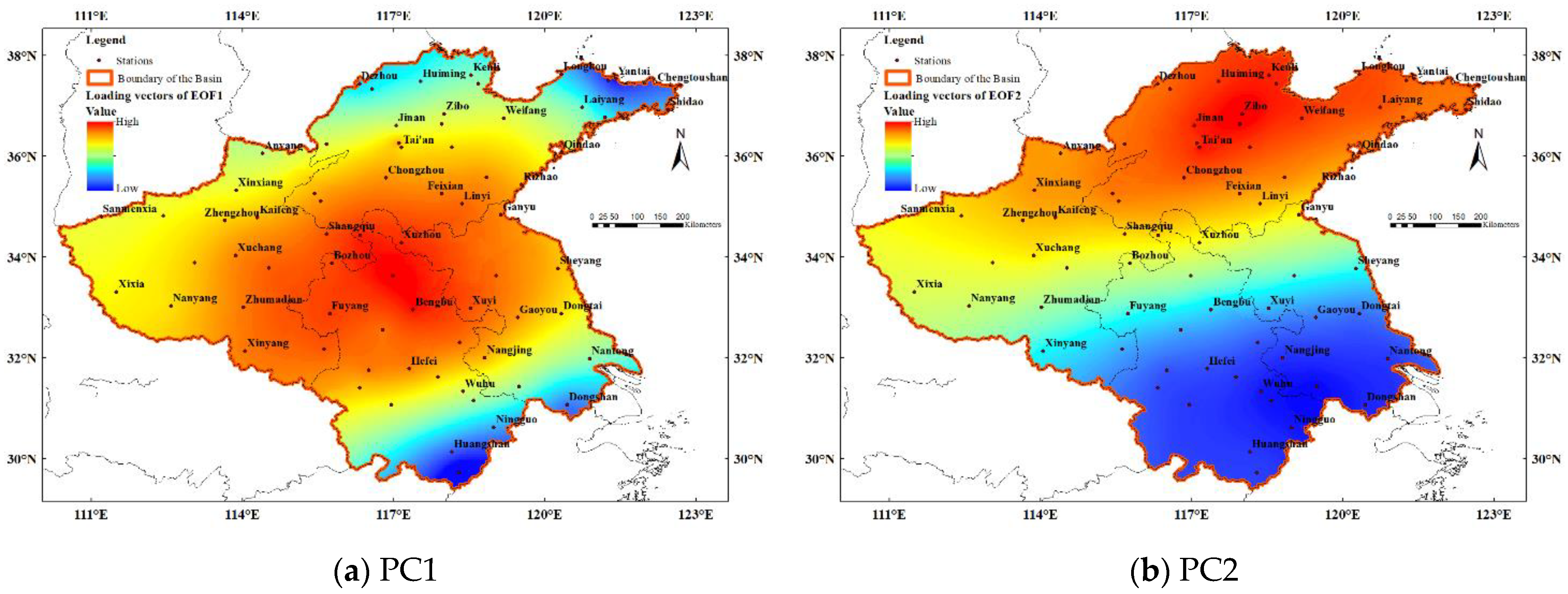
• The spatial variability in the Huaihe River Basin seems to be localized well with three distinct sub-regions regarding seasonal drought and monthly drought. There are two sub-regions that can account for spring and winter drought variability, respectively, referring to the middle part of the study area (occupying most areas of the river basin) and the north part of the river basin.
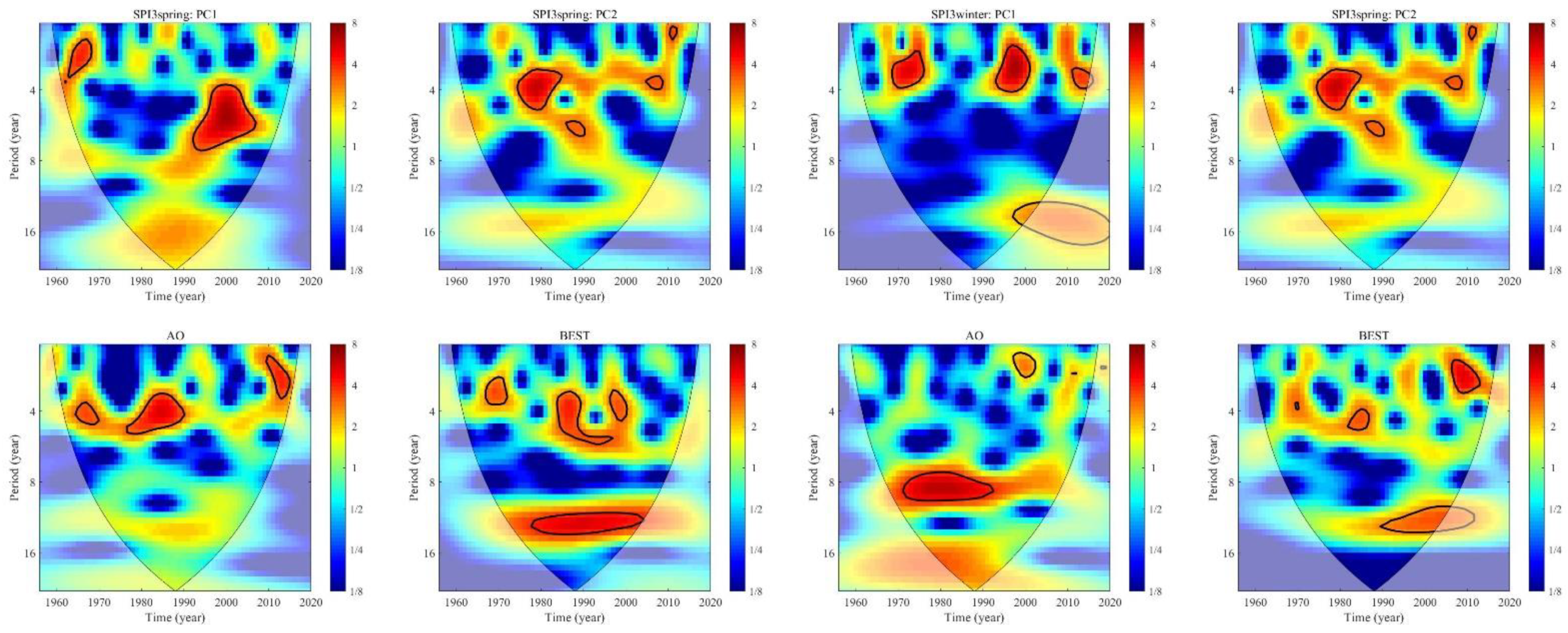
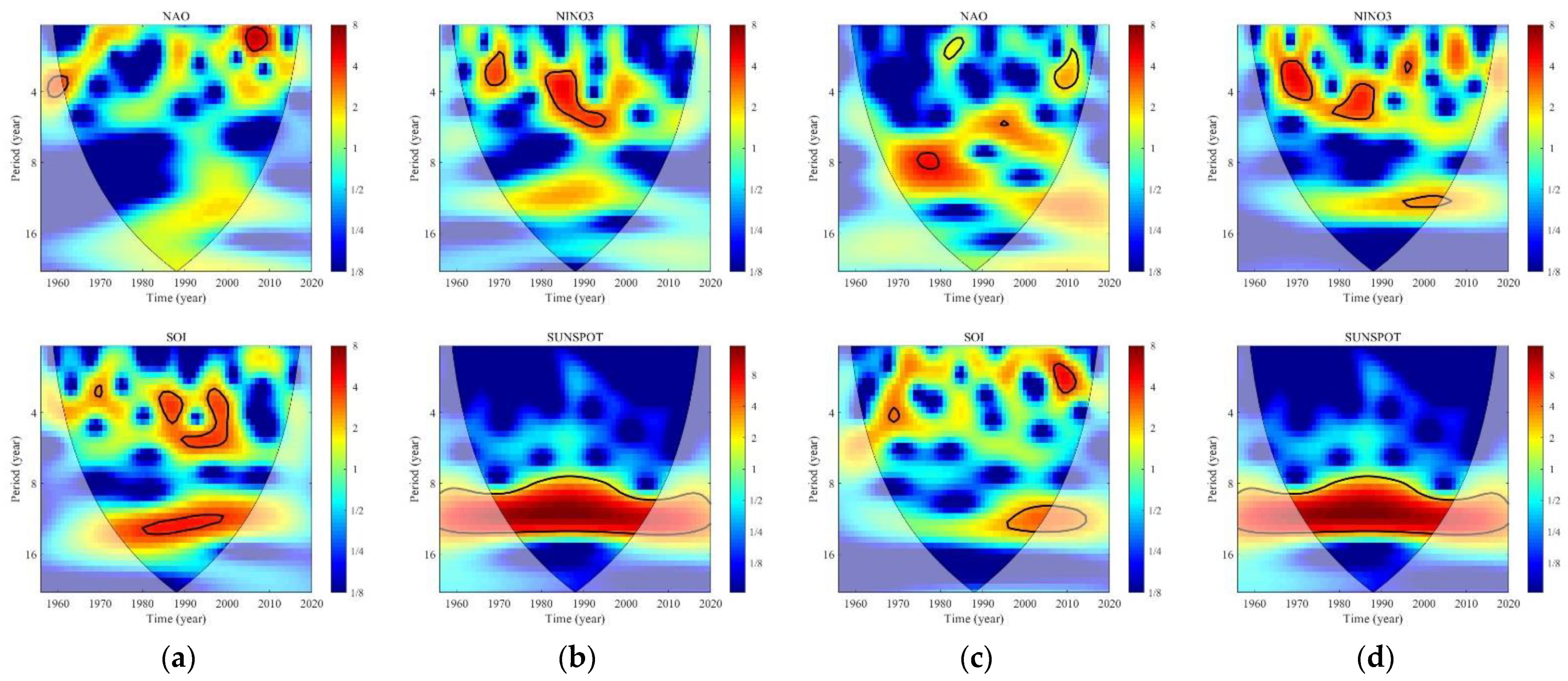
• Spring and winter droughts fluctuate with a 2–7-year cycle in the time series, especially in terms of concurrence. The periodical oscillation features of winter PC1, referring to the 2–4-year cycle from 1969 to 1976, during the periods of 1992–2001 and 2011–2015, closely resemble those of the BEST, Niño3, and SOI series. The periodicity of spring PC1, characterized by the 3.5–7-year cycle during 1992–2008 and the 2–3-year cycle from 1965 to 1968, has good consistency with the NAO and SOI series.
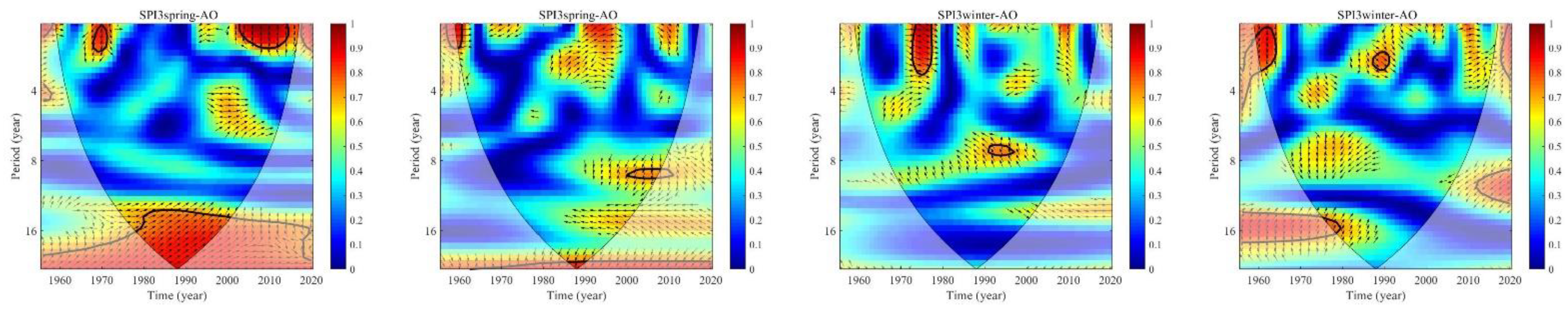
• There are in-phase multi-scale relations between spring/winter PC1 and the AO, BEST, and Niño3, of which the climate indices lead spring PC1 by 1.5–2 years and the climate indices lag winter PC1 by 1.5–3 years. Anti-phase multi-scale relations between spring PCs and the SOI were observed. The sunspot number shows weak anti-phase relations with spring PCs and weak in-phase relations with winter PCs, always with a 2-year lead period (spring/winter PC1) or a 2-year lag (spring PC2). Moreover, the NAO has an important impact on the interdecadal variation in the two spring PCs, while the AO and Niño3 mainly affect the interannual scale. Niño3 and the SOI are intimately related to the two winter PCs around the interdecadal scales covering the 8–12-year cycle.
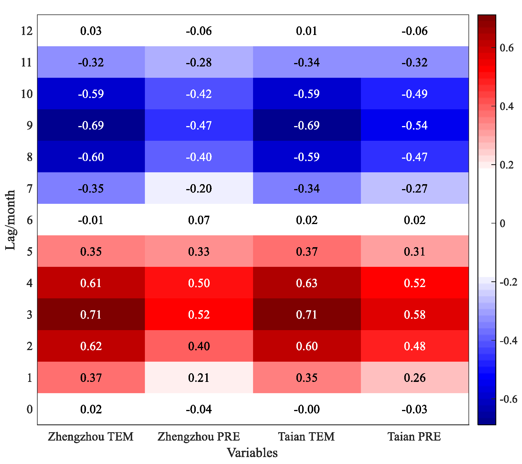
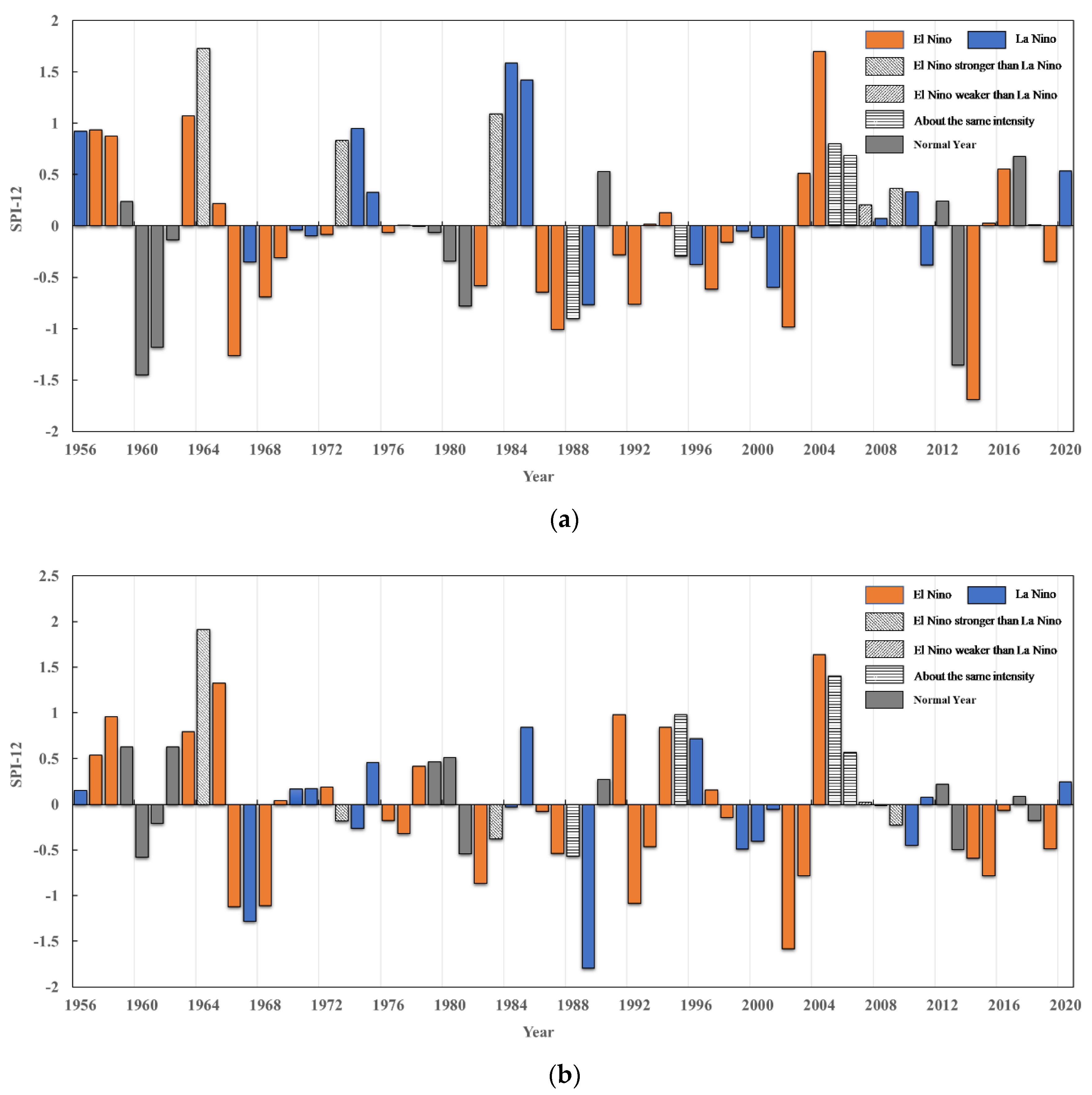
• Taking Zhengzhou City and Taian City in the Huaihe River Basin as representative stations, the monthly average temperature and the monthly average precipitation lag Niño3 by 3 months with a significant positive relation, while both lag Niño3 by 9 months with a significant negative relation. The onset, process, and intensity of El Niño/La Niña events clearly influenced the dryness/wetness condition in the river basin.

The results presented in this paper could contribute a lot to our understanding of the multi-scale linkages between drought and large-scale climate phenomena in the Huaihe River Basin. They provide a possible way to improve the accuracy of drought prediction by taking the NAO, the AO, and Niño3 as predictors for spring drought and Niño3 and the SOI as predictors for winter drought. Moreover, we provided a preliminary discussion of the feedback between drought/flooding and atmospheric circulation. Thus, the information could serve as a basis for water resource planning and management in the river basin and for making emergency plans for drought events.

However, the obtained results from the observed data are not suitable for extrapolation into the future [57,58]. On the one hand, the statistical results could be related to climate variability but not to persistent changes in time. On the other hand, the investigated trend depends on the observation period, so it could be different if the observation period is extended. With the decrease in precipitation in the northern part of the river basin and the increase in precipitation in other parts of the river basin over the past 65 years, it would be worth determining in future work exactly what the influence of the changing climate on drought in the river basin is and how it is affected.

References

1. Intergovernmental Panel on Climate Change (IPCC). The Sixth Assessment Report (AR6); IPCC: Geneva, Switzerland, 2021. [Google Scholar]
2. Gong, Y.; Jiang, T.; Su, B.; Huang, J.; Kundzewicz, Z.W.; Jing, C.; Sun, H. Synchronous characteristics of precipitation extremes in the Yangtze and Murray-Darling River Basins and the role of ENSO. J. Meteorol. Res. 2021, 35, 282–294. [Google Scholar] [CrossRef]
3. Jin, Z.; Tao, S. Study on the relationship between ENSO cycle and summer and winter precipitation in eastern China. Chin. J. Atmos. Sci. 1999, 23, 663–672. [Google Scholar]
4. Liu, Z.Z.; Zhang, X.; Fang, R.H. Multi-scale linkages of winter drought variability to ENSO and the Arctic Oscillation: A case study in Shaanxi, North China. Atmos. Res. 2018, 200, 117–125. [Google Scholar] [CrossRef]
5. Nugroho, A.R.; Tamagawa, I.; Harada, M. The Relationship between River Flow Regimes and Climate Indices of ENSO and IOD on Code River, Southern Indonesia. Water 2021, 13, 1375. [Google Scholar] [CrossRef]
6. Yao, R.; Xia, M.; Sun, P.; Wen, Q.; Liu, G.; Liang, Y. Spatio-temporal distribution characteristics of meteorological drought and climate influence factors. Acta Ecol. Sin. 2021, 41, 337–347. [Google Scholar]
7. Kong, F.; Shi, P.; Fang, J.; Lv, L.; Fang, J.; Guo, J. Advances and prospects of spatiotemporal pattern variation of extreme precipitation and its affecting factors under the background of global climate change. J. Catastrophol. 2017, 32, 165–174. [Google Scholar] [CrossRef]
8. Liu, Y.; Ding, Y. Effect of ESNO event on seasonal precipitation and temperature in China. Sci. Atmos. Sin. 1995, 19, 2. [Google Scholar]
9. Sang, Y. Improvement on Wavelet Analysis Methodology and Its Application in Hydrologic Times Series Analysis and Forecasting. Ph.D. Thesis, Nanjing University, Nanjing, China, 2011. [Google Scholar]
10. Wang, Y.; Zhang, Q.; Zhang, S.; Chen, X. Spatial and temporal characteristics of precipitation in the Huaihe river basin and its response to ENSO events. Sci. Geogr. Sin. 2016, 36, 128–134. [Google Scholar] [CrossRef]
11. Chen, Y.; Ma, S.; Xu, J.; Guo, W.; Jia, Y.; Zhao, T. Analysis on climate change and related factors in north China in recent 65 years. J. Hebei Norm. Univ. Nat. Sci. 2021, 45, 314–324. [Google Scholar] [CrossRef]
12. Liu, S.; Lang, X.; Jiang, D. Time-varying responses of dryland aridity to external forcings over the last 21 ka. Quat. Sci. Rev. 2021, 262, 106989. [Google Scholar] [CrossRef]
13. Wang, W.; Xu, H. The modification of Palmer Drought Severity Index in the research of drought in Huaihe area. Adv. Earth Sci. 2012, 27, 60–67. [Google Scholar]
14. Byakatonda, J.; Parida, B.P.; Moalafhi, D.B.; Kenabatho, P.K. Analysis of long term drought severity characteristics and trends across semiarid Botswana using two drought indices. Atmos. Res. 2018, 213, 492–508. [Google Scholar] [CrossRef]
15. Karoly, D.J.; Braganza, K. Identifying global climate change using simple indices. Geophys. Res. Lett. 2001, 28, 2205–2208. [Google Scholar] [CrossRef]
16. Khan, S.; Piao, S.; Zheng, G.; Khan, I.U.; Bradley, D.; Khan, S.; Song, Y. Sea Surface Temperature Variability over the Tropical Indian Ocean during the ENSO and IOD Events in 2016 and 2017. Atmosphere 2021, 12, 587. [Google Scholar] [CrossRef]
17. Towner, J.; Ficchí, A.; Cloke, H.L.; Bazo, J.; Coughlan de Perez, E.; Stephens, E.M. Influence of ENSO and tropical Atlantic climate variability on flood characteristics in the Amazon basin. Hydrol. Earth Syst. Sci. 2021, 25, 3875–3895. [Google Scholar] [CrossRef]
18. Li, C.; Luo, D.; Fang, Z.; Zhou, H. Linkage of Inter-decadal Variations of the Arctic Oscillation and Summer Precipitation over North China. J. Nanjing Inst. Meteorol. 2005, 28, 755–762. [Google Scholar]
19. Tang, J. Relation between rainfall of Shaanxi Province and activities of sunspot based on ensemble empirical mode decomposition. J. Arid Land Resour. Environ. 2017, 31, 154–159. [Google Scholar]
20. Zeng, W.; Yu, Z.; Li, X. The influence of elevation, latitude and Arctic Oscillation on trends in temperature extremes over northeastern China, 1961–2011. Meteorol. Atmos. Phys. 2017, 130, 191–209. [Google Scholar] [CrossRef]
21. Chen, J.; Chung, C. Representation of global precipitation anomalies using four major climate patterns. Sci. China Technol. Sci. 2015, 58, 927–934. [Google Scholar] [CrossRef]
22. Baawain, M.S.; Nour, M.H.; El-Din, A.G.; El-Din, M.G. El Niño southern-oscillation prediction using southern oscillation index and Niño3 as onset indicators: Application of artificial neural networks. J. Environ. Eng. Sci. 2005, 4, 113–121. [Google Scholar] [CrossRef]
23. Li, C.; Li, G. The NPO/NAO and interdecadal climate variation in China. Adv. Atmos. Sci. 2000, 17, 555–561. [Google Scholar] [CrossRef]
24. Wahiduzzaman, M. Major Floods and Tropical Cyclones over Bangladesh: Clustering from ENSO Timescales. Atmosphere 2021, 12, 692. [Google Scholar] [CrossRef]
25. Sobral, B.S.; de Oliveira-Júnior, J.F.; de Gois, G.; Pereira-Júnior, E.R.; Terassi, P.M.d.B.; Muniz-Júnior, J.G.R.; Lyra, G.B.; Zeri, M. Drought characterization for the state of Rio de Janeiro based on the annual SPI index: Trends, statistical tests and its relation with ENSO. Atmos. Res. 2019, 220, 141–154. [Google Scholar] [CrossRef]
26. Zou, L.; Xia, J.; Zhang, Y. Spatio-temporal evolution of extreme precipitation in the middle and lower reaches of the Yangtze River. Resour. Environ. Yangtze Basin 2021, 30, 1264–1274. [Google Scholar] [CrossRef]
27. Wang, J.; Sun, C.; Zheng, Z.; Li, X. Drought characteristics of the Loess Plateau in the past 60 years and its relationship with changes in atmospheric circulation. Acta Ecol. Sin. 2021, 41, 5340–5351. [Google Scholar] [CrossRef]
28. Xu, Q.; Chen, L.; Fan, Y.; Tang, W.; Lu, B. Relationship between drought characteristics and climate index in Lanzhou based on SPEI index. J. China Hydrol. 2021, 41, 56–62. [Google Scholar] [CrossRef]
29. Chen, S.; Ju, Q.; Hao, Z.; Wang, L.; Xu, H. Analysis of Extreme Hydrometeorological Characteristics in Huaihe River Basin in Recent 70 Year. J. Hebei Univ. Eng. Nat. Sci. Ed. 2020, 37, 75–83. [Google Scholar] [CrossRef]
30. Lin, H.; Wang, J.; Huang, J.; Jiang, C. Climate drought in Huai River Basin under climate change. China Rural Water Hydropower 2020, 6, 21–35. [Google Scholar]
31. Yan, S.; Weng, B.; Jing, L.; Li, M. Spatial and Temporal Distribution Characteristics of Droughts in Huaihe River Basin. China Rural Water Hydropower 2021, 4, 160–165. [Google Scholar]
32. Lu, Y.; Yan, D.; Qin, T.; Song, Y.; Weng, B.; Yuan, Y.; Dong, G. Assessment of Drought Evolution Characteristics and Drought Coping Ability of Water Conservancy Projects in Huang-Huai-Hai River Basin, China. Water 2016, 8, 378. [Google Scholar] [CrossRef] [Green Version]
33. Ji, C.; Ma, H.; Peng, Y.; Li, N. Prediction of meteorological drought in Huai river basin considering multiple climatic indices. China Rural Water Hydropower 2021, 4, 16–21. [Google Scholar]
34. Cheng, Y.; Plag, H.-P.; Hamlington, B.D.; Xu, Q.; He, Y. Regional sea level variability in the Bohai Sea, Yellow Sea, and East China Sea. Cont. Shelf Res. 2015, 111, 95–107. [Google Scholar] [CrossRef]
35. Ning, T.; Feng, Q.; Li, Z.; Li, Z. Recent changes in climate seasonality in the inland river basin of Northwestern China. J. Hydrol. 2020, 590, 15212. [Google Scholar] [CrossRef]
36. Zhang, L.; Shi, R.; Fraedrich, K.; Zhu, X. Enhanced joint effects of ENSO and IOD on Southeast China winter precipitation after 1980s. Clim. Dyn. 2021. [Google Scholar] [CrossRef]
37. WMO. International Meteorological Vocabulary, 2nd ed.; WMO: Geneva, Switzerland, 1992. [Google Scholar]
38. McKee, T.B.; Doesken, N.J.; Kieist, J. The Relationship of Drought Frequency and Duration to Time Scales. In Proceedings of the 8th Conference on Applied Climatology, Boston, MA, USA, 17–22 January 1993; pp. 179–184. [Google Scholar]
39. Xie, W.S.; Tian, H.; Wang, S.; Tang, W. Study on spatial-temporal charasteristics of drought in Huaihe River Basin based on CI index. Meteorol. Mon. 2013, 39, 1171–1175. [Google Scholar]
40. Husak, G.J.; Michaelsen, J.; Funk, C. Use of the gamma distribution to represent monthly rainfall in Africa for drought monitoring applications. Int. J. Climatol. 2007, 27, 935–944. [Google Scholar] [CrossRef]
41. Sun, Q.; Xu, G.; Ma, C. Study on the characteristics of drought in Haikou City based on standardized precipitation index. South-North Water Transf. Water Sci. Technol. 2018, 16, 58–65. [Google Scholar] [CrossRef]
42. Torrence, C.; Compo, G.P. A practical guide to wavelet analysis. Bull. Am. Meteorol. Soc. 1998, 79, 61–78. [Google Scholar] [CrossRef] [Green Version]
43. Torrence, C.; Webster, P. Interdecadal changes in the ESNO monsoon system. J. Clim. 1999, 12, 2679–2690. [Google Scholar] [CrossRef] [Green Version]
44. Grinsted, A.; Moore, J.C.; Jevrejeva, S. Application of the cross wavelet transform and wavelet coherence to geophysical time series. Nonlinear Process. Geophys. 2004, 11, 561–566. [Google Scholar] [CrossRef]
45. Wen, K.G.; Bian, G.H. Chinese Meteorological Disaster Code: Jiangsu Province; China Meteorological Press: Beijing, China, 2008; pp. 191–201. [Google Scholar]
46. Wen, K.G.; Pang, T.H. Chinese Meteorological Disaster Code: Henan Province; China Meteorological Press: Beijing, China, 2005; pp. 98–127. [Google Scholar]
47. Wen, K.G.; Zhai, W.Q. Chinese Meteorological Disaster Code: Anhui Province; China Meteorological Press: Beijing, China, 2007; pp. 181–211. [Google Scholar]
48. Xin, Z.; Xie, Z. Influence of ENSO event on precipitation in Huaihe River basin. Sci. Atmos. Sin. 2005, 25, 346–354. [Google Scholar]
49. Qian, Y.; Wang, Q.; Huang, D. Studies of floods and droughts in the Yangtze-Huaihe River basin. Chin. J. Atmos. Sci. 2007, 31, 1279–1288. [Google Scholar]
50. Murphy, B.F.; Timbal, B. A review of recent climate variability and climate change in southeastern Australia. Int. J. Climatol. 2008, 28, 859–879. [Google Scholar] [CrossRef]
51. Nistor, M.-M.; Dezsi, Ş.; Cheval, S.; Baciu, M. Climate change effects on groundwater resources: A new assessment method through climate indices and effective precipitation in Beliş district, Western Carpathians. Meteorol. Appl. 2016, 23, 554–561. [Google Scholar] [CrossRef]
52. Renard, B.; Thyer, M. Revealing Hidden Climate Indices from the Occurrence of Hydrologic Extremes. Water Resour. Res. 2019, 55, 7662–7681. [Google Scholar] [CrossRef]
53. Schepen, A.; Wang, Q.J.; Robertson, D. Evidence for Using Lagged Climate Indices to Forecast Australian Seasonal Rainfall. J. Clim. 2012, 25, 1230–1246. [Google Scholar] [CrossRef]
54. Li, X.; Zhai, P. On indices and indicators of ENSO episodes. Acta Meteorol. Sin. 2000, 58, 102–109. [Google Scholar]
55. Xu, W.; Ma, J.; Wang, W. A review of studies on the influence of ENSO events on the climate in China. Sci. Meteorol. Sin. 2005, 25, 212–220. [Google Scholar]
56. Lenssen, N.J.L.; Goddard, L.; Mason, S. Seasonal Forecast Skill of ENSO Teleconnection Maps. Weather Forecast. 2020, 35, 2387–2406. [Google Scholar] [CrossRef]
57. Bloschl, G.; Hall, J.; Viglione, A.; Perdigao, R.A.P.; Parajka, J.; Merz, B.; Lun, D.; Arheimer, B.; Aronica, G.T.; Bilibashi, A.; et al. Changing climate both increases and decreases European river floods. Nature 2019, 573, 108–111. [Google Scholar] [CrossRef] [PubMed]
58. De Luca, D.L.; Petroselli, A.; Galasso, L. A Transient Stochastic Rainfall Generator for Climate Changes Analysis at Hydrological Scales in Central Italy. Atmosphere 2020, 11, 1292. [Google Scholar] [CrossRef]
Figure 1. Geophysical location and the topographical distribution of the Huaihe River Basin. The background map is the world physical map from the Environmental Systems Research Institute (ESRI).
Atmosphere 12 01446 g001
Figure 2. Spatial patterns of the first two EOF modes of seasonal SPI-3: (a) represents the first EOF modes of seasonal SPI-3 and (b) represents the second EOF modes of seasonal SPI-3.
Atmosphere 12 01446 g002aAtmosphere 12 01446 g002b
Figure 3. Spatial patterns of the first two EOF modes of SPI-1: (a) represents PC1 and (b) represents PC2.
Atmosphere 12 01446 g003
Figure 4. The continuous wavelet power spectrum for the (a,b) spring and (c,d) winter time series of PC1, PC2, and six climate indices. The figures are color-mapped to indicate a high degree of wavelet coherence in red and yellow and a low degree of coherence in blue. The thick contours designate the 95% confidence level against red noise. The black line is the cone of influence (COI).
Atmosphere 12 01446 g004aAtmosphere 12 01446 g004b
Figure 5. The wavelet coherence between climate indices and (a) Spring-PC1, (b) Spring-PC2, (c) Winter-PC1, and (d) Winter-PC2. The figures are color-mapped to indicate a high degree of wavelet coherence in red and yellow and a low degree of coherence in blue. The thick contours designate the 95% confidence level against red noise. The black line is the cone of influence (COI).
Atmosphere 12 01446 g005aAtmosphere 12 01446 g005b
Figure 6. The cross-wavelet spectrum of climate indices and (a) Spring-PC1, (b) Spring-PC2, (c) Winter-PC1, and (d) Winter-PC2. The figures are color-mapped to indicate a high degree of wavelet coherence in red and yellow and a low degree of coherence in blue. The thick contours designate the 95% confidence level against red noise. The black line is the cone of influence (COI).
Atmosphere 12 01446 g006aAtmosphere 12 01446 g006b
Figure 7. The distribution of the total number of drought events (SPI <= −1) from 1956 to 2020. The dark purple points represent meteorology stations, and the size of each point is equivalent to the total number of drought events. The bigger the point is, the more drought events occurred.
Atmosphere 12 01446 g007
Figure 8. The correlation coefficient of monthly average temperature/precipitation and Niño3.
Atmosphere 12 01446 g008
Figure 9. The relations between SPI-12 and El Niño/La Niña events in (a) Zhengzhou City and (b) Taian City during 1956–2020. The years that El Niño and La Niña events occurred come from an integration of statistics from several research references [34,54,55,56].
Atmosphere 12 01446 g009