Review

Turbulence: Vertical Shear of the Horizontal Wind, Jet Streams, Symmetry Breaking, Scale Invariance and Gibbs Free Energy

Physics Department, Imperial College London, London SW7 2AZ, UK
Atmosphere 2021, 12(11), 1414; https://doi.org/10.3390/atmos12111414
Submission received: 7 September 2021 / Revised: 25 October 2021 / Accepted: 26 October 2021 / Published: 27 October 2021
(This article belongs to the Special Issue Structure of Atmospheric Turbulence)

Abstract

:
The increase of the vertical scaling exponent of the horizontal wind Hv(s) with altitude from the surface of the Pacific Ocean to 13 km altitude, as observed by GPS dropsondes, is investigated. An explanation is offered in terms of the decrease of gravitational force and decrease of quenching efficiency of excited photofragments from ozone photodissociation with increasing altitude (decreasing pressure). Turbulent scaling is examined in both the vertical from dropsondes and horizontal from aircraft observations; the scaling exponents H for both wind speed and temperature in both coordinates are positively correlated with traditional measures of jet stream strength. Interpretation of the results indicates that persistence of molecular velocity after collision induces symmetry breaking emergence of hydrodynamic flow via the mechanism first modelled by Alder and Wainwright, enabled by the Gibbs free energy carried by the highest speed molecules. It is suggested that the combined effects have the potential to address the cold bias in numerical models of the global atmosphere.

1. Introduction

Atmospheric turbulence is a very large field, as an exploration on Web of Science with that as the search term will reveal—27 new hits in the first 11 days of June 2021, and many thousands since 1950. It affects most aspects of the atmosphere, from modelling for weather forecasting, through water transport, cloud formation, radiative transfer, biogeospheric exchanges, pollutant transport and deposition to such engineering activities as aviation, wind turbines, adaptive optics for astronomical telescopes and building construction. These processes are all involved in global heating and the evolution of macroweather, the climate and their modelling.
This review will have a narrow focus, on turbulence as a fundamental part of atmospheric dynamics and will be confined to the scale invariant, statistical multifractal approach originated by Schertzer and Lovejoy [1,2] and described at book length by Lovejoy and Schertzer [3] and by Lovejoy [4]. A molecular viewpoint on this approach has been derived from observational analysis of airborne data [5,6] and is employed here. No single cut-off date is applied; the arguments in references [7,8] will be taken as having established 23/9-dimensional scaling in the atmosphere on both observational [7,9,10,11] and theoretical [8] grounds. Attention will be focussed on the unexplained result of the change in scaling exponents of horizontal wind speed with altitude from the surface to 13 km altitude over the Pacific Ocean [12] and also for the lower stratospheric jet streams [13]. The scaling exponents in the jet streams are correlated with conventional measures of jet stream strength, both vertically and horizontally [5,6,10,12,13]. As a consequence of the analysis, the cold bias in numerical models of the global atmosphere is also potentially addressable.

2. Observations of the Vertical Scaling of the Horizontal Wind Speed

The result addressed in this article is displayed in Figure 1. The data are from 315 GPS dropsondes released by the NOAA G4 research aircraft over the eastern Pacific Ocean in the area bounded by (21–60° N, 128–172° W) during January, February and March 2006; similar data were acquired during 2004 and 2005 [5,6,10,11,12]. The feature to which attention is paid here is the systematic increase with altitude in the value of Hv(s) the scaling exponent in the vertical of the horizontal wind speed, s. H is defined in equations given in references [5,6,12]. There was no theoretical explanation offered for this increase in [12] beyond a remark that the presence of jet streams in the upper troposphere and lower stratosphere may have caused statistical inhomogeneity.
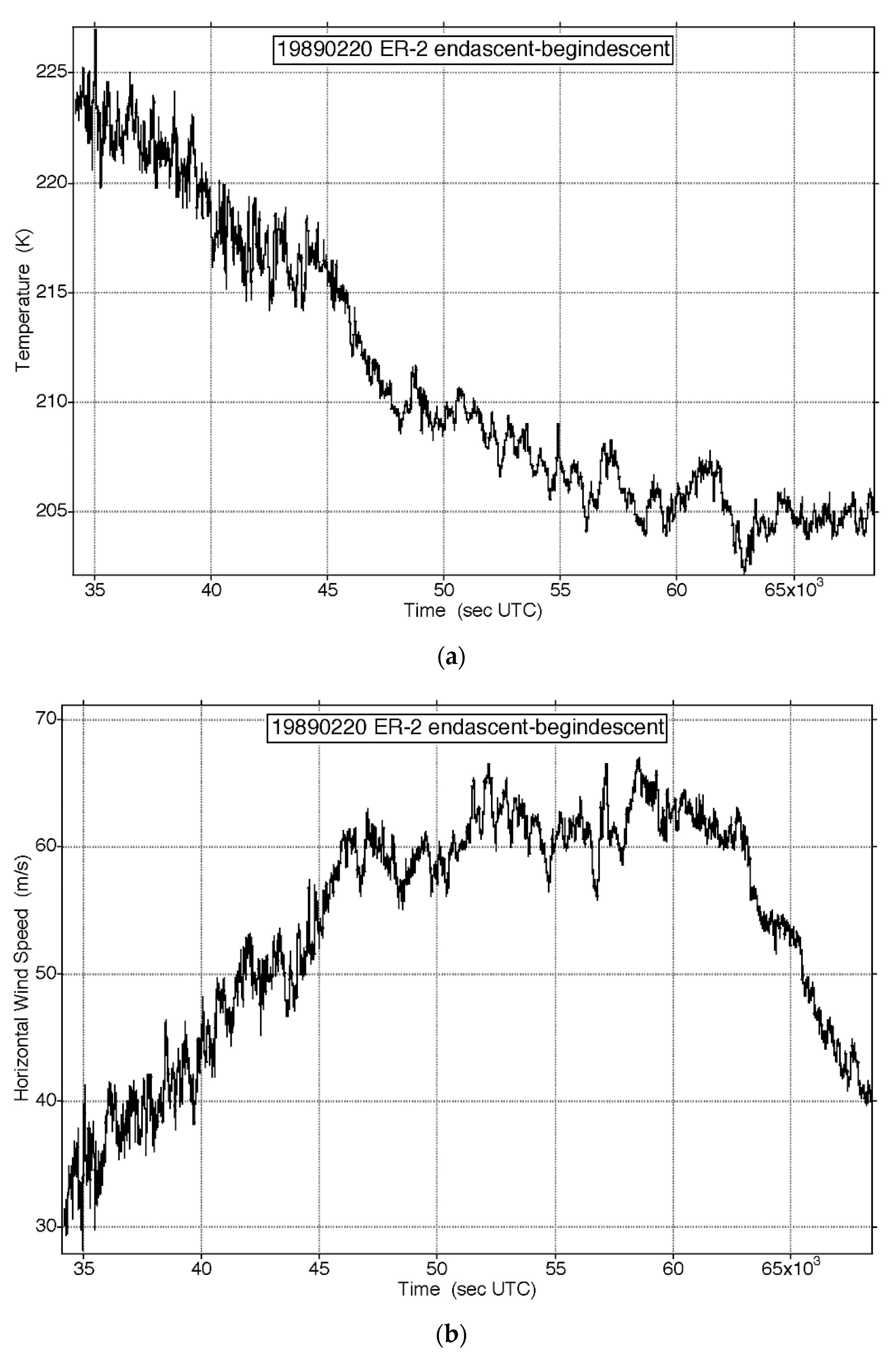
We commence by displaying in Figure 2a,b traces of the temperature and wind speed at 1 Hz from the NASA ER-2 aircraft along the lower stratospheric polar night jet stream 19890220 (yyyymmdd format). This is the longest flight leg available, over one Earth radius [5,13]. Additionally, shown in Figure 2c are the corresponding wind and shear vectors averaged at 8192, 1024 and 128 s intervals; the aircraft flies at a true air speed of 200 ms
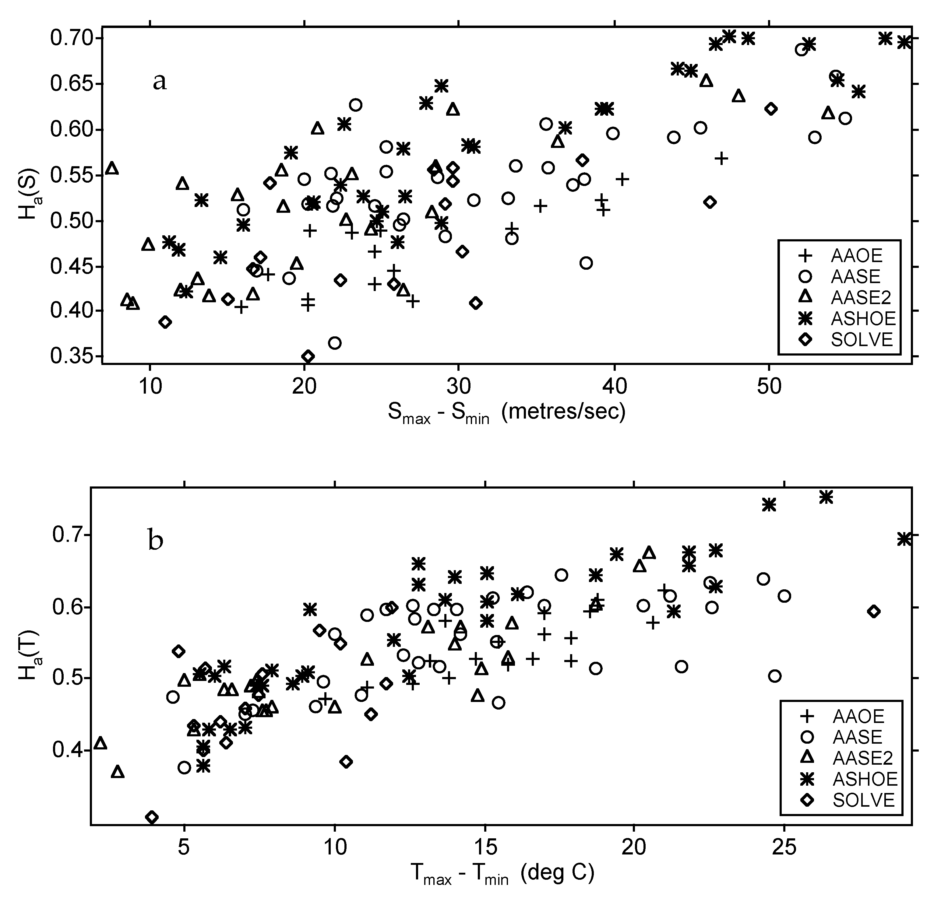
−1. Similar data from all qualifying ER-2 flight legs 1987–2000 are used to plot the values of H(T) and H(s) against traditional horizontal measures of jet stream strength, the cross-jet (meridional) temperature gradient and the horizontal wind shear, respectively, see Figure 3a,b. Note the positive correlations in each case.
The particular horizontal examples in Figure 2 are extended by plotting the vertical Hv exponents for horizontal wind speed against the vertical wind shear and vertical depth as measured by the dropsondes, traditional measures of jet stream strength. There is a positive correlation in each case. Thus, in both the horizontal and the vertical the scaling H exponents show positive correlations with traditional measures of jet stream strength.

3. Interpretation of the Observed Turbulence

While it is evident from Figure 2, Figure 3 and Figure 4 that jet stream structure is turbulent, variable and scale invariant over the whole range from 40m to 7 × 10⁶ m (about one Earth radius), it is clear that the scaling exponent of the horizontal wind is correlated with traditional meteorological measures of jet stream strength in both the horizontal and vertical. The scaling exponent H(s) is less along the jet than across it, see Figure 5 and reference [13]. That result may be interpreted as meaning that speed shear is more efficient at lowering H, that is to say decreasing organized flow and increasing ‘mixing’ or dissipation than is directional wind shear; it produces anticorrelation on all scales. Note that H = 1 corresponds to perfect neighbour-to-neighbour correlation, while H = 0 corresponds to perfect neighbour-to-neighbour anticorrelation on all scales.
An approximate diagnostic formulation of why in meteorological terms the vertical scaling exponent of the horizontal wind speed increases with height may be found in the synoptic saying “the westerlies increase with height because it’s colder toward the pole”, expressed mathematically in the thermal wind equation [14]:
V g / p = ( g / f ) k   ×   p ( h / p )   =   ( R / f p ) k   ×   p T
or
Vg/z = (g/fT)k × ∇pT
Here, Vg is geostrophic wind, p is pressure, g is the gravitational force, f = 2Ωsinφ, Ω is the Earth’s rotation rate, φ is latitude, k is the unit vector in the vertical, ∇p is the pressure gradient, h is height and R is the ideal gas constant. For further discussion, see [14].
There are component relations involved in (1) and (2). If Earth’s mean radius is a, and geometric altitude is z, then the radial distance r from the planetary centre is r = a + z.
The hydrostatic relation may be written as
gz/p = −1/ρ = −RT/p
where ρ is density.
Note that
gg* + Ω2kr
where g* = g0/(1 + z/a)2 and kr is the unit position vector from the air under consideration to the axis of rotation. g0 is the mean gravitational constant at mean sea level.
A further form of (1) may be written by defining geopotential Φ(z) at height z as
Φ     0 z g d z
  • so, dΦ = −(RT/p)dp = −RTdlnp
  • and Φ(z1) − Φ(z2) = R p ( 2 ) p ( 1 ) T d l n p
  • from which geopotential height Z is defined as
Z = Φ(z)/g0
and the thermal wind equation may then be written
VTh = (1/f)k × ∇(Φ1Φ2)
Consider each variable in (1) in the light of the change of scaling of the horizontal wind speed in Figure 1. The gravitational force decreases with height by a small but significant amount in accordance with (2). References [5,15,16,17] advanced the idea of the possibility that the rotational degrees of freedom of the nitrogen and oxygen molecules of the air had non-Maxwell–Boltzmann occupancies, altering the specific heat at constant pressure. That possibility exists because of the observed correlation between the ozone photodissociation rate and the intermittency of temperature. That effect would result in translationally hot O atomic and O2 molecular photofragments causing non-equilibrium probability distributions of translational and rotational degrees of freedom in the ‘thermal bath’ of air molecules. Such a condition would alter the perspective of the molecular definition of temperature itself [5,6].
The phenomenon we are examining may also be formulated on a molecular basis as well as in the above meteorological terms. The basis used follows reference [18]. Variables are formatted as is conventional for physicochemical treatments.
At steady state for 1 mole of air
dlnC/dz= −Mg/RT
where C is the concentration of air in moles per litre at altitude z. Substituting mN0 = M where N0 is Avogadro’s number, M is the molar weight, m is the molecular weight of air and the volume of air between levels z1 and z2 is assumed to be at steady state (the upward pressure is balanced by the downward force of gravity). Then, integrating between levels 1 and 2
ln(C2/C1) = N0mg(z1z2)/RT
As g decreases and T increases with altitude (especially in the stratosphere relative to an ‘equilibrium’ T with Maxwell–Boltzmann speed distributions) so (z1z2) must increase. Although the aircraft data are limited to 20 km altitude, the effect will be to make the air warmer than its equilibrium value at a given altitude. Such an effect may be expected to amplify with altitude, as collisional quenching of the excited states becomes less effective at lower pressures. At the same time, gravitational force g is decreasing with altitude; both it and pressure decrease from the surface to the stratopause at 50 km. The combined effect is of the right sign to address the cold bias in global atmospheric models that is particularly evident in the stratosphere [6].
Operating via the mechanism calculated by Alder and Wainwright [19], hydrodynamic flow becomes evident as a symmetry breaking phenomenon progressing from initiation at the microscale through the mesoscale [20] to the macroscale. Such symmetry breaking is often, but not always, accompanied by a dynamical phase change; those phase changes would show up in the scale invariance analysis as changes of slope in the log–log plots. The flow will be turbulent and scale invariant [21] and will violate the assumptions made in formulating numerical models of the atmosphere [6]. We note that the initiating mechanism for the Alder and Wainwright mechanism is the persistence of molecular velocity after collision [22]. That implies that in local thermodynamic equilibrium, Maxwellian and gaussian statistics are not accurate and become less so as altitude increases. The overpopulation of high-speed molecules carries the Gibbs free energy that enables the requisite work, and is evident in the fat tails of the probability distributions of temperature and wind speed. The air is neither completely organized (H = 1) or completely random (H = 0).
The persistence ratio w12 is the ratio of the mean velocity after collision to that before collision between molecules of masses m1 and m2 and is given by
w 12   =   1 2 m 1 + 1 2 ( m 1 ) 2 ( m 2 ) 1 / 2 ln [ ( ( m 2 ) + 1 ) / ( m 1 ) 1 / 2 ]
If m1 = m2 then w12 is 0.406, but for different molecular weights the heavier molecule will be slowed less than the lighter one. The physical effect is to spontaneously break the symmetry of a volume of gas, which has randomized molecular velocities, because such a volume has continuous translational symmetry. In a gas in an anisotropic location, which air volumes invariably are, the Alder–Wainwright mechanism will be initiated and hydrodynamic flow will emerge. The translationally hot photofragments from ozone photodissociation via the Hartley, Huggins, Chappuis and Wulf bands that stretch from the UV to the near IR will reinforce the tendency. The observed scale invariant turbulence has a different, lower symmetry.
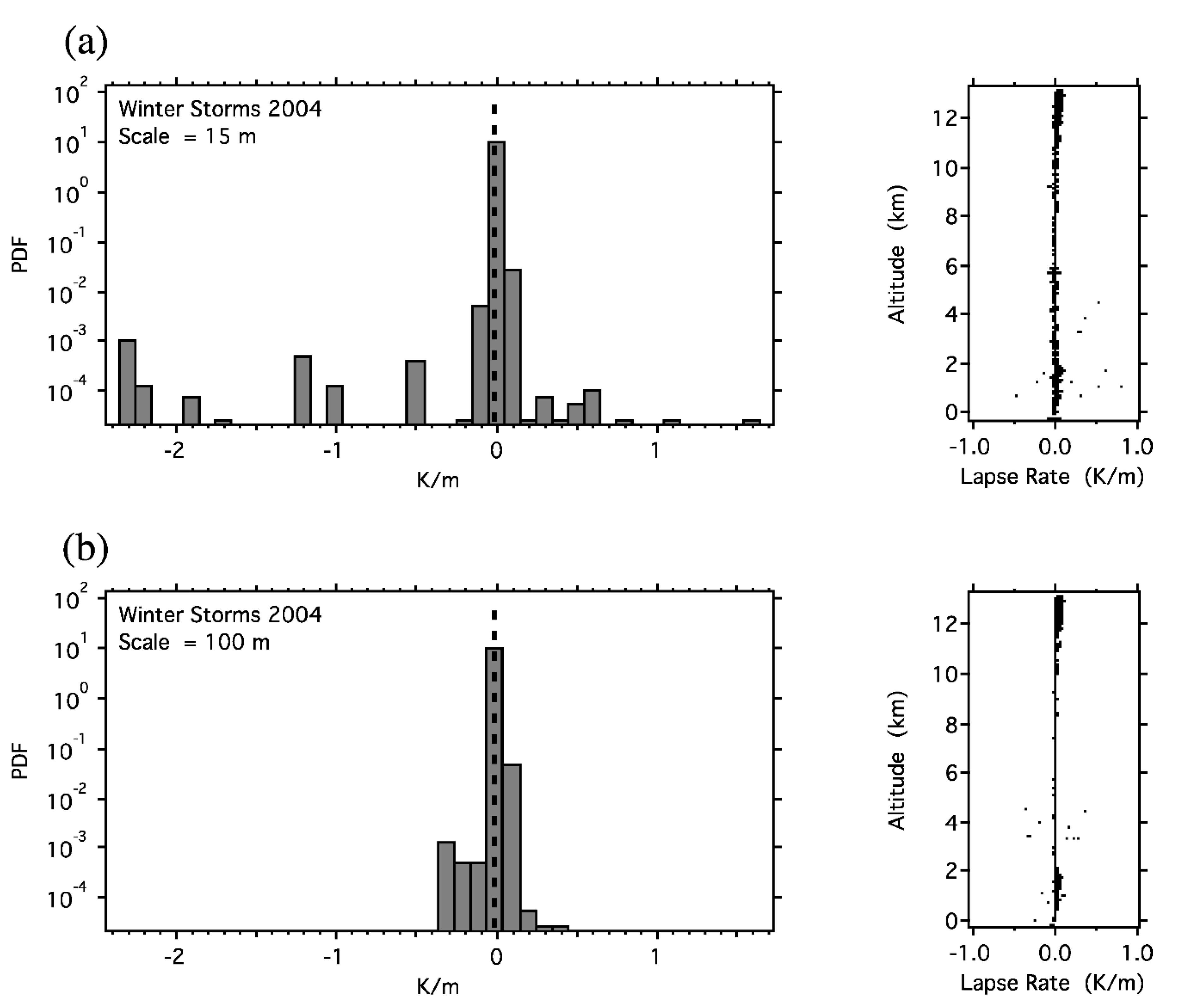
The effects of turbulent structure upon the dry adiabatic lapse rate (DALR) are evident in Figure 6. At vertical scales less than about 30 m the frequency of occurrence of the condition DALR > 9.8 K km−1 is no different above and below the tropopause, with about 1% of cases exceeding it at scales below 15 m; they are convectively unstable. By extrapolation, about 50% exceedance of the DALR occurs at 93 cm.

4. Conclusions

A case has been presented that the effect of molecular behaviour in a weakening gravitational field and decreasing pressure as altitude increases results in the increase in Hv(s), the vertical scaling of the horizontal wind observed in Figure 1. Persistence of velocity after collision and the emergence of hydrodynamic flow spontaneously break the continuous translational symmetry of the random molecular motion underlying the theory of Maxwell–Boltzmann distributions. In turn, that will devalue attempts to deploy higher symmetries to the atmosphere, such as Fourier analysis and wave formulations, which seek to impose a symmetry on the air that it does not have. Scale invariance is the lower symmetry induced by the symmetry breaking induction of turbulence rooted in persistence of molecular velocity after collision and the Alder–Wainwright mechanism. The scaling of the dropsonde temperature data shows that at a vertical scale of 100 m the tropopause is visible in the context of exceedance of the dry adiabatic lapse rate, but is not at scales less than 30 m. The scaling exponents of the horizontal wind across and along the polar night jet streams indicate that speed shear is more effective than directional shear at producing anticorrelation in neighbouring intervals-mixing-on all scales. The translational excitation of ozone photofragments will increase the translational energy of all air molecules as altitude increases, as the ozone photodissociation rate increases in the enhanced solar photon flux. Especially in the stratosphere, these effects could address the cold bias in numerical models of the global atmosphere [24]. This hypothesis could be tested by dropping GPS sondes from large constant level balloons from up to 40 km altitude and applying the multifractal analysis used here. Note that the enhanced stratospheric cooling from increasing CO2 can counteract the increased heating from more ozone heating as the CFC burden decreases. In any event, these processes must be represented on a secure molecular basis. Finally, we recall that Gibbs free energy, carried by the fastest moving molecules and derived from the entropy difference between the incoming solar beam from a 5800 K source and the outgoing infrared flux over the whole 4π solid angle from a source at 255 K to the 2.7 K temperature of space, is the driving force for the development of turbulence by symmetry breaking [17]. More is indeed different [25]. Note that the unresolved issue as to whether atmospheric turbulence was Kolmogorov (isotropic) or not for adaptive optics in ground based astronomical telescopes [26] has been resolved in favour of anisotropy, see Figure 1. As has been argued earlier [17], turbulence in the atmosphere will need to be addressed by molecular dynamics from the smallest scales up rather than by seeking to impose inappropriate symmetries on the so far analytically insoluble Navier–Stokes equation.

Funding

This research received no external funding.

Institutional Review Board Statement

Not applicable.

Informed Consent Statement

Not applicable.

Data Availability Statement

NASA Airborne Data Repository.

Conflicts of Interest

The author declares no conflict of interest.

References

  1. Schertzer, D.; Lovejoy, S. The dimension and intermittency of atmospheric dynamics. In Turbulent Shear Flows; Springer: New York, NY, USA, 1985; Volume 4, pp. 7–33. [Google Scholar]
  2. Schertzer, D.; Lovejoy, S. Physical modeling and analysis of rain and clouds by anisotropic scaling multiplicative processes. J. Geophys. Res. D 1987, 92, 9693–9714. [Google Scholar] [CrossRef]
  3. Lovejoy, S.; Schertzer, D. The Weather and Climate: Emergent Laws and Multifractal Cascades; Cambridge University Press: Cambridge, UK, 2013; ISBN 978-1-107-01898-3. [Google Scholar]
  4. Lovejoy, S. Weather, Macroweather and the Climate; Oxford University Press: Oxford, UK, 2019; ISBN 978-0-19-086421-7. [Google Scholar]
  5. Tuck, A.F. Atmospheric Turbulence: A Molecular Dynamics Perspective; Oxford University Press: Oxford, UK, 2008; ISBN 978-0-19-923653-4. [Google Scholar]
  6. Tuck, A.F. From molecules to meteorology via turbulent scale invariance. Q. J. R. Meteorol. Soc. 2010, 136, 1125–1144. [Google Scholar] [CrossRef]
  7. Lovejoy, S.; Tuck, A.F.; Schertzer, D.; Hovde, S.J. Reinterpreting aircraft measurements in anisotropic scaling turbulence. Atmos. Chem. Phys. 2009, 9, 5007–5025. [Google Scholar] [CrossRef] [Green Version]
  8. Schertzer, D.; Tchiguirinskaia, I.; Lovejoy, S.; Tuck, A.F. Quasi-geostrophic turbulence and generalized scale invariance, a theoretical reply. Atmos. Chem. Phys. 2012, 12, 327–336. [Google Scholar] [CrossRef] [Green Version]
  9. Pinel, J.; Lovejoy, S.; Schertzer, D.; Tuck, A.F. Joint horizontal-vertical anisotropic scaling, isobaric and isoheight statistics from aircraft data. Geophys. Res. Lett. 2012, 39, L11803. [Google Scholar] [CrossRef] [Green Version]
  10. Lovejoy, S.; Tuck, A.F.; Hovde, S.J.; Schertzer, D. Do stable atmospheric layers exist? Geophys. Res. Lett. 2008, 35, L01802. [Google Scholar] [CrossRef] [Green Version]
  11. Lovejoy, S.; Tuck, A.F.; Schertzer, D. The horizontal cascade structure of atmospheric fields determined from aircraft data. J. Geophys. Res. D 2010, 115, D13105. [Google Scholar] [CrossRef]
  12. Hovde, S.; Tuck, A.F.; Lovejoy, S.; Schertzer, D. Vertical scaling of temperature, wind and humidity fluctuations: Dropsondes from 13 km to the surface of the Pacific Ocean. Int. J. Remote Sens. 2011, 32, 5891–5918. [Google Scholar] [CrossRef]
  13. Tuck, A.F.; Hovde, S.J.; Bui, T.P. Scale invariance in jet streams: ER-2 data around the lower-stratospheric polar night vortex. Q. J. R. Meteorol. Soc. 2004, 130, 2423–2444. [Google Scholar] [CrossRef]
  14. White, A.A. A view of the equations of meteorological dynamics and various approximations. In Large-Scale Atmosphere-Ocean Dynamics I; Norbury, J., Roulstone, I., Eds.; Cambridge University Press: Cambridge, UK, 2002; Chapter 1; pp. 1–100. [Google Scholar]
  15. Tuck, A.F.; Hovde, S.J.; Richard, E.C.; Gao, R.-S.; Bui, T.P.; Swartz, W.H.; Lloyd, S.A. Molecular velocity distributions and generalized scale invariance in the turbulent atmosphere. Faraday Discuss. 2005, 130, 181–193. [Google Scholar] [CrossRef] [PubMed]
  16. Tuck, A.F. Scale Invariant Turbulence and Gibbs Free Energy in the Atmosphere. In Entropy and Exergy in Renewable Energy; Wang, L.-S., Ed.; IntechOpen: London, UK, 2020; Chapter NN. [Google Scholar] [CrossRef]
  17. Tuck, A.F. Theoretical chemistry and the calculation of the atmospheric state. Atmosphere 2021, 12, 727. [Google Scholar] [CrossRef]
  18. Moelwyn-Hughes, E.A. Physical Chemistry, 2nd ed.; Pergamon Press: Oxford, UK, 1961; Chapter 1. [Google Scholar]
  19. Alder, B.J.; Wainwright, T.E. Decay of the velocity autocorrelation function. Phys. Rev. 1970, 1, 18–21. [Google Scholar] [CrossRef]
  20. Laughlin, R.B.; Pines, D.; Schmalian, J.; Stojkovic, B.P.; Wolynes, P. The middle way. Proc. Natl. Acad. Sci. USA 2000, 97, 32–37. [Google Scholar] [CrossRef] [PubMed] [Green Version]
  21. Kadau, K.; Barber, J.L.; Germann, T.C.; Holian, B.L.; Alder, B.J. Atomistic methods in fluid simulation. Philos. Trans. R. Soc. A 2012, 368, 1547–1560. [Google Scholar] [CrossRef] [PubMed] [Green Version]
  22. Chapman, S.; Cowling, T.G. The Mathematical Theory of Non-Uniform Gases, 3rd ed.; Cambridge University Press: Cambridge, UK, 1970. [Google Scholar]
  23. Lovejoy, S.; Tuck, A.F.; Hovde, S.; Schertzer, D. Is isotropic turbulence relevant in the atmosphere? Geophys. Res. Lett. 2007, 34, L15802. [Google Scholar] [CrossRef]
  24. Polichtchouk, I.; Stockdale, T.; Bechtold, P.; Diamantakis, M.; Malardel, S.; Sandu, I.; Vána, F.; Wedi, N. Control on Stratospheric Temperature in IFS: Resolution and Vertical Advection. ECMWF Technical Memorandum no. 847. ECMWF 2019. [Google Scholar] [CrossRef]
  25. Anderson, P.W. More is different—Broken symmetry and the nature of the hierarchical structure of science. Science 1972, 177, 393–396. [Google Scholar] [CrossRef] [PubMed] [Green Version]
  26. Bradford, L.W.; Flatter, S.M.; Max, C.E. Modelling atmospheric turbulence effects on a ground-based interferometer. In Proceedings of the Volume 2200, Amplitude and Intensity: Spatial Interferometry II, Kailua, Kona, HI, USA, 9 June 1994. [Google Scholar]
Figure 1. The vertical scaling exponent H of the horizontal wind from 315 GPS dropsondes released from the NOAA G4 aircraft flying at approximately 13 km in the area bounded by (21–60° N, 128–172° W). The lines are root mean square fits to the vertical shear across layers, increasing logarithmically upwards, and are labelled by the corresponding value of H. The data for each level are offset by one order of magnitude, to aid legibility. The reference lines refer to what different theories predict: 1 is gravity waves, 3/5 is Bolgiano–Obukhov, 1/3 is Kolmogorov. Bolgiano–Obukhov is a reasonable fit in the lower troposphere, but H increases to values near 0.75 at 12.5 km., where jet streams were often observed. Isotropy (Kolmogorov) is nowhere observed. Equations defining H may be found in references [5,6,12].
Atmosphere 12 01414 g001
Figure 2. (a) Observations of temperature at 1 Hz frequency from the ER-2 aircraft flying at 200 ms−1 at approximately 20 km altitude for 10 h 15 m on 19890220 (yyyymmdd), into a headwind of the polar night jet stream, which was aligned between (59° N, 6° E) and (38° N, 75° W). The fluctuations are atmospheric variability, and the instrumental noise is insignificant. (b) The horizontal wind speed corresponding to the temperature measurements in (a). Again, instrumental noise is not evident. (c) The horizontal wind shear vectors derived from the observations in (b), averaged over three intervals differing by a factor of eight. The directions vary over 360° and unidirectional flow at uniform velocity is nowhere evident. That behaviour is typical of the 140 ER-2 flight segments obtained during polar ozone missions from 1987 to 2000.
Atmosphere 12 01414 g002aAtmosphere 12 01414 g002b
Figure 3. (a) Scaling exponent H for the horizontal wind speed obtained from the ER-2 plotted against the difference between the maximum and minimum wind speeds measured by the aircraft in crossing the polar night jet stream. (b) The same flights, but for temperature. For both wind speed and temperature, there is a positive correlation between H and traditional measures of jet stream strength, the horizontal gradients of wind speed and temperature.
Atmosphere 12 01414 g003
Figure 4. Left, vertical scaling exponent H from GPS dropsondes released from the NOAA G4 aircraft flying at 13 km over the northeastern Pacific Ocean, Winter Storms missions 2004, 2005, 2006 [12], plotted against the depth of the jet stream observed by the sondes. STJ, subtropical jet stream; PFJ, polar front jet stream; SPNJ, stratospheric polar night jet stream. Right, H for horizontal wind speed observed from the dropsondes plotted against the vertical difference between the maximum and minimum wind speeds seen by the sondes.
Atmosphere 12 01414 g004
Figure 5. Upper, H for wind speed observed from the ER-2 during flight along the Arctic polar night jet stream, 19890220, the same flight as in Figure 2. It is one of the few along rather than across the jet, and has the lowest value of H recorded. Lower, the highest value of H encountered by the ER-2, cross-jet over Antarctica in October 1994.
Atmosphere 12 01414 g005
Figure 6. (a) Probability distribution functions (ordinate) versus dry adiabatic lapse rate (abscissa) from GPS dropsondes released by the NOAA G4 aircraft from 13 km over the north-eastern Pacific Ocean during the Winter Storms 2004 mission [5,10,23], data at 15 m resolution. (b) Same data at 100 m resolution.
Atmosphere 12 01414 g006
Publisher’s Note: MDPI stays neutral with regard to jurisdictional claims in published maps and institutional affiliations.

