The UrbEm Hybrid Method to Derive High-Resolution Emissions for City-Scale Air Quality Modeling

Abstract

As cities are growing in size and complexity, the estimation of air pollution exposure requires a detailed spatial representation of air pollution levels, rather than homogenous fields, provided by global- or regional-scale models. A critical input for city-scale modeling is a timely and spatially resolved emission inventory. Bottom–up approaches to create urban-scale emission inventories can be a demanding and time-consuming task, whereas local emission rates derived from a top–down approach may lack accuracy. In the frame of this study, the UrbEm approach of downscaling gridded emission inventories is developed, investing upon existing, open access, and credible emission data sources. As a proof-of-concept, the regional anthropogenic emissions by Copernicus Atmospheric Monitoring Service (CAMS) are handled with a top–down approach, creating an added-value product of anthropogenic emissions of trace gases and particulate matter for any city (or area) of Europe, at the desired spatial resolution down to 1 km. The disaggregation is based on contemporary proxies for the European area (e.g., Global Human Settlement population data, Urban Atlas 2012, Corine, OpenStreetMap data). The UrbEm approach is realized as a fully automated software tool to produce a detailed mapping of industrial (point), (road-) transport (line), and residential/agricultural/other (area) emission sources. Line sources are of particular value for air quality studies at the urban scale, as they enable explicit treatment of line sources by models capturing among others the street canyon effect and offer an overall better representation of the critical road transport sector. The UrbEm approach is an efficient solution for such studies and constitutes a fully credible option in case high-resolution emission inventories do not exist for a city (or area) of interest. The validity of UrbEm is examined through the evaluation of high-resolution air pollution predictions over Athens and Hamburg against in situ measurements. In addition to a better spatial representation of emission sources and especially hotspots, the air quality modeling results show that UrbEm outputs, when compared to a uniform spatial disaggregation, have an impact on NO₂ predictions up to 70% for urban regions with complex topographies, which corresponds to a big improvement of model accuracy (FAC2 > 0.5), especially at the source-impacted sites.

1. Introduction

The percentage of the population residing in urban areas in Europe continues to increase from 74.9% in 2019; it is expected to reach 77.5% (83.7%) by 2030 (2050) [1,2]. In turn, this will increase the urban population exposed to air pollutants and the consequent health impacts. Presently, despite past reductions in emissions that have taken place in most European countries, a significant proportion of the urban population in the EU-28 is still exposed to concentrations of certain air pollutants above the EU limit values. This is even more so when the more stringent WHO air quality guideline values are taken into account (i.e., the percentage population exposure to PM_2.5 above limit values rises from 6–8% (EU limit) to 74–81% (WHO limit). With respect to PM₁₀, the respective exceedances were 13–19% (42–52%), for surface O₃, they were 12–29% (95–98%), and for NO₂, they were 7–8% both for the EU and WHO [3]. The estimated premature deaths in the 27 EU Member States and the United Kingdom attributed to PM_2.5, NO₂, and O₃ exposure are 374,000, 68,000, and 14,000, respectively, while the number of years of life lost (YLL) per 100,000 inhabitants is estimated at 800, 100, and 30 [3]. The ever-rising amount of evidence regarding the negative effects of air pollution on health—evidence assessed as having high or moderate certainty of an association between a pollutant and a specific health outcome—has led to new and even more stringent guidelines set by the WHO in September 2021 [4].

As cities are growing in size and feature inherent complexity, urban air quality management requires a more detailed spatial representation of air pollution levels than given by (a) the available number of stationary measurement stations and (b) the current resolution (one to tens of kilometers) provided by regional Eulerian grid air pollution models [5]. These models, inter alia, fail to capture concentration gradients that typically occur near heavily trafficked streets [6], with further implications on exposure [7] and the choice of mitigation measures. The accuracy of the assessment of the effectiveness of these measures is dependent on the robustness of the emission (the flux of certain trace gases and particles into the atmosphere) inventories and their efficacy for scenario analysis to assess measures for emission reductions and improved air quality [8,9]. Therefore, emission inventories are considered a key component in an urban air quality management plan [10]. Emission inventories come at various scales, from global to regional and local. For the purposes of this study, we will only consider the latter two and, in particular, how well they serve the urban domain, as it is there where urban health studies are often hindered by the lack of city-scale emission inventories.

Several regional emission inventories exist in Europe, with spatial resolution usually between 7 and 11 km. A spatial inter-comparison of some of these top–down and proxy-based inventories, including EDGAR v4.3.1, TNO-MACCIII, EMEP, and JRC07, has been performed in representative European urban areas [11], and sources herein. The authors acknowledge that although bottom–up inventories do often exist for major cities, providing more accurate information at a higher spatial resolution is still of utmost importance to be able to rely on consistent and harmonized European-wide inventories for extensive air quality modeling. However, the study also identified significant differences between regional emission inventories in these cities due to the choices made in terms of the disaggregation approach in the industrial sector, where the use of the population density as a proxy for the diffuse fraction results in an over-allocation of emissions in urban areas and in the residential sector, where spatial patterns and variation of emissions from wood and coal burning are not captured.

As noted in Kadaverugu et al. [12], CTMs require emission inventories representative of the study area. Similarly, appropriate spatial and temporal resolution inventories on a grid that is compatible with city-scale models is imperative. Currently, many countries provide emission inventories down to 1 × 1 km² [10], although no universal standards are available; thus, applications rely on urban or local-scale project initiatives [5]. The Forum for Air Quality Modeling (FAIRMODE) has recently published a report providing recommendations to build emissions for fine-scale applications [13]. This report advocates for an expansion of the existing EMEP/EEA [14] emission guidance document to ensure that spatial disaggregation approaches provide appropriate results for local/urban emission assessments, for an adoption of the Gridded Nomenclature For Reporting (GNFR) and for national efforts toward urban-scale emission compilation following bottom–up approaches.

A bottom–up approach relies mostly on local activity estimates collected over the area of interest (e.g., traffic counts for road segments in a city). One recent example, albeit more generalized, was the approach followed by Guevara et al. [15] where, in sync with EMEP guidelines, a method for estimating and preparing high-resolution bottom–up emissions from multiple anthropogenic sources in a flexible and transparent way was developed. The approach presents a Europe-wide applicability as long as the required input data are available. A top–down approach, on the other hand, distributes emission totals spatially (country or region, e.g., derived from total fuel sales) according to gridded proxies (e.g., population, land use). Nevertheless, bottom–up approaches have usually different levels of detail or granularity, as not all parameters needed for a pure bottom–up approach are known and, as a result, bottom–up and top–down modeling approaches are often combined [10].

Given the fact that bottom–up inventories are resource intensive and are not built in a standardized manner [16], methodological homogeneity between different cities and overall compliance with AQ Directives is not easily achieved. Moreover, bottom–up approaches are in general site-specific and resource intensive, so the support for their compilation in a consistent basis does not exist for every city. For this, we developed a hybrid and modular approach to enable the construction of the desired high-resolution emission fields. The approach is hybrid, as it commences from downscaling regional emission inventories to a gridded inventory—in this case, the CAMS-REG regional inventories from the Copernicus Atmospheric Monitoring Service (CAMS) [17,18], following a traditional top–down methodology. However, instead of disaggregating solely into areas, it explicitly handles the—critical for the urban environment—line and point sources, so as to accommodate for urban CTM models such as [19,20,21,22]. The approach is also modular as it can handle different proxies for spatially disaggregating the regional inventory, in this case JRC’s Global Human Settlement Layer (GHSL) [23], Copernicus Land Monitoring Services’ Corine Land Cover (CLC) [24], European Pollutant Release and Transfer Register (E-PRTR) point source information (https://industry.eea.europa.eu/, accessed: 23 October 2021), and Open Street Map (OSM) [25] road network data.

This study describes the framework for creating emission inventories for urban air quality simulations across Europe by utilizing generic and publicly available proxies in a consistent manner. While the concept of downscaling coarser emissions, up to the 1 km mark, by utilizing proxies (point, line, or areas) has been visited in the past, such as in the MEGAPOLI project (https://cordis.europa.eu/project/id/212520, accessed: 23 October 2021), where a fine emission inventory was created for the whole of Germany albeit though localized data and effort, here, Europe-wide applicability, consistency, and ease of use were the strategic objectives. The demonstration cities are Hamburg and Athens, i.e., cities with different climatic, geomorphological, and urban growth characteristics, where the accuracy of the produced inventories is evaluated by comparing concentration fields from urban-scale air quality modeling with actual measurements. This framework is completely scalable, sustainable, has a low computational and overall implementation cost, and is of high and critical importance for air quality modelers, especially when national/local emission data are either unavailable or outdated.

The development of the city-scale emission inventories is based on a hybrid approach, investing upon existing, open access, and credible emission datasets. Their spatial disaggregation is based on contemporary spatial datasets of the European area (Section 2.1). The emission inventories and spatial datasets are processed in the newly developed UrbEm framework (Section 2, Figure 1), which is a hybrid method to derive high-resolution emissions for city-scale air quality modeling. UrbEm is fully automated to produce a detailed mapping of industrial (point), transport (line), residential, agricultural, and other (area) emission sources for any city (or area) of Europe at the desired spatial analysis. These products can be directly used as input for local-scale atmospheric models, for the estimation of air pollution levels within the region of study, at high resolution. In this study, we use emission inventories that were downscaled with the presented approach in the chemistry transport model EPISODE-CityChem [22] and applied it to two European urban areas, Athens (Greece) and Hamburg (Germany). Finally, the results of the emissions downscaling procedure and their application in EPISODE-CityChem are presented (Section 3.1), evaluated (Section 3.2), and discussed (Section 4).

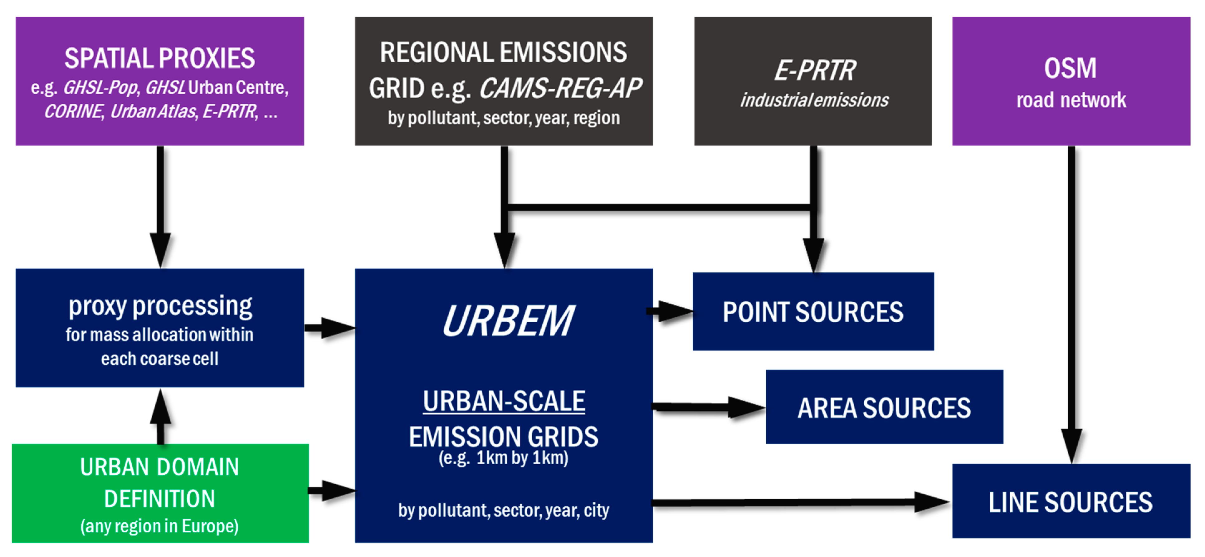
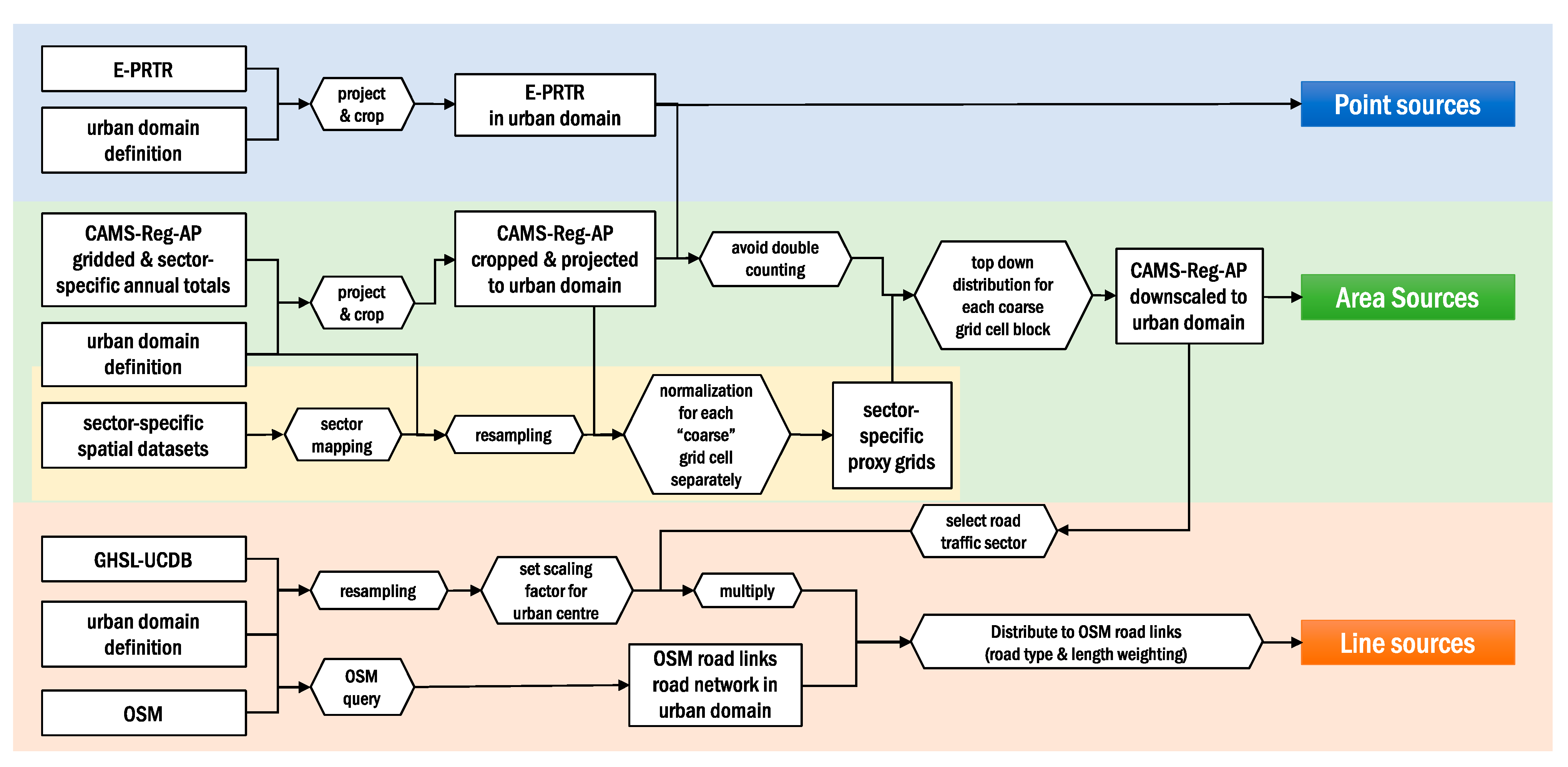
2. The UrbEm Approach for Emissions Downscaling

The developed hybrid approach to arrive at high-resolution area emissions, as well as point and line source emissions for city-scale air quality modeling, follows the generalized framework described in Figure 1. This framework can be applied to any urban region in Europe. Based on an urban domain definition, in line with the requirements of a city-scale air quality model, sector-specific spatial proxies are prepared based on publicly available datasets to distribute CAMS-REG and E-PRTR emission datasets to area, point, and line sources. The overall methodology includes first the general approach to prepare spatial proxies for different sectors (2.1) and second, the application of these proxies in the hybrid-downscaling approach, which is called UrbEm (2.2). A reduced overview on the general methodology is illustrated in Figure 1, while a more detailed insight in the realization of the general methodology is given in Figure 2.

The application of the UrbEm approach is realized as a software tool that is open source distributed via GitHub (https://github.com/martinottopaul/UrbEm, accessed: 23 October 2021). There are two different versions available: (1) based on the interpreted programming language R [26], and (2) a combination of Python (https://www.python.org, accessed: 23 October 2021). Both solutions run on different operating systems on single-core processors and need a minimum of 2 gigabyte RAM. Depending on the extent of the model domain and its resolution, the preparation of proxies, the downscaling of emissions, and the creation of point, area, and line source output files, the required computing time is about 30–45 min (for example, for a 50 km × 50 km domain, with a grid resolution of 1 km × 1 km, including 15,000 line source elements and several point sources).

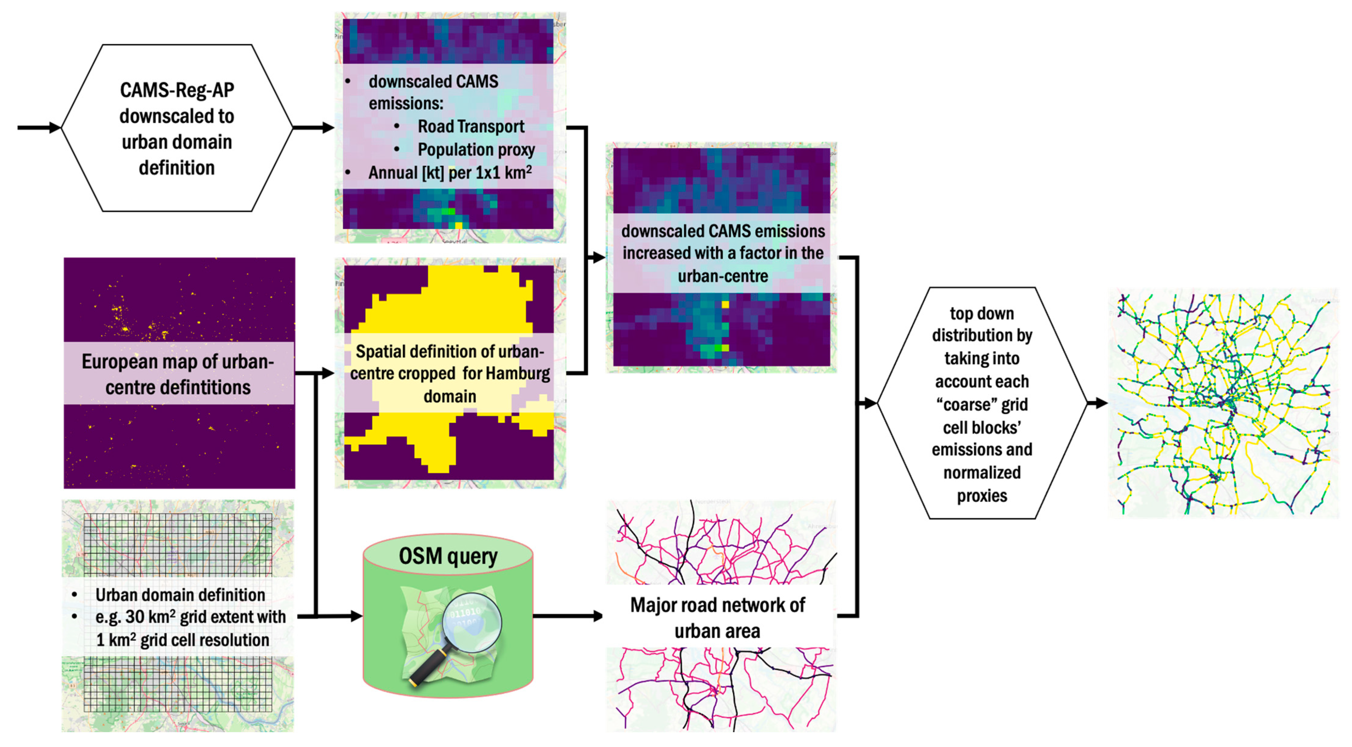
2.1. Spatial Datasets: Selection and Processing

As illustrated in Figure 1 and Figure 2, the spatial disaggregation of the selected CAMS regional emission inventory CAMS-REG (≈6 × 6 km² grid cells) [17] is performed with sector-specific spatial proxies. These proxies are prepared with publicly available, well-established, contemporary spatial datasets of European (or Global) coverage (for a detailed description of all datasets, see Appendix A). In a first step, suitable spatial datasets are mapped to sectors following SNAP or GNFR nomenclature.

Table 1. The spatial proxies (and their origin) used to disaggregate each anthropogenic activity (expressed as source sectors in SNAP and GNFR) in the proposed downscaling framework. More information on all spatial datasets used can be found in Appendix A.

Anthropogenic Activity (Source Sector)	Spatial Proxy (Dataset Source)
Public Power and Refineries (SNAP 1 * or GNFR A)	Polygons hosting Public Power installations (E—PRTR and CLC 2018) combined with Land type characterized as ‘Industry’ (CLC 2018)
Residential Heating (SNAP 2 or GNFR B)	(Residential) population Density (GHS-POP 2015)
Fossil Fuel Production and Fugitive (SNAP 5 or GNFR D)	Land type characterized as ‘Industry’ (CLC 2018)
Solvent and Other Use Production (SNAP 6 or GNFR E)	(Residential) population Density (GHS-POP 2015)
Road Emissions (SNAP 7: 71,72,73,74,75 or GNFR F)	Major Road Network (OSM) ** consisting of highways, trunks, primary and secondary roads, and their links
Non-Road Mobile Emissions (SNAP8): Shipping (GNFR G)	A superposition of Global shipping routes (CIA 2013) and Land type characterized as ‘Ports’ (CLC 2018)
Non-Road Mobile Emissions (SNAP8): Aviation (GNFR H)	Land type characterized as ‘Airports’ (CLC 2018)
Non-Road Mobile Emissions (SNAP8): Off Road Machinery (GNFR I)	Land type characterized as ‘Non-Road Mobile Sources’ (CLC 2018) relevant to agricultural, industrial, and construction activities
Waste Treatment (SNAP 9 or GNFR J)	Polygons hosting waste management installations (E—PRTR and CLC 2018) combined with Land type characterized as ‘Agriculture’ (CLC 2018) to allocate open waste
Agriculture (SNAP 10 or GNFR K and GNFR L)	Land type characterized as ‘Agriculture’ (CLC 2018)
Industrial Combustion and Processes (SNAP 34 or GNFR B)	Polygons hosting installations of mineral or chemical industries and of production (and processing) of wood, paper, metals, animal and vegetable (E—PRTR and CLC 2018) combined with Land type characterized as ‘Industry’ (CLC 2018)

* CAMS-REG v.1 (SNAP categorization) uses point sources for the spatial allocation of industrial installations. ** OSM data are periodically (30 days) retrieved to ensure consistency with the frequent official updates of the database.

introduces anthropogenic activities based on SNAP or GNFR classification, which are allocated to the appropriate proxies, such as population density, land type categories (e.g., industrial, agriculture), and road networks.

Population density, as provided within the GHSL-POP layer, is used as a spatial proxy to distribute emissions from residential heating and the use of solvents. The residential population density, mapped for 2015 in 1 km² spatial resolution, is retrieved from the Global Human Settlement Layer [23].

The CORINE land use/cover (LULC) dataset is used as a spatial proxy for the majority of source sectors (Table 1) [24]. Original LULC gridded data for 2018, with the spatial resolution of 100 m and 44 land types, are aggregated to 1 km² and reclassified into 12 generalized land types. Reclassified gridded data are either used as spatial proxies for sectors, such as industry and agriculture, or combined with other spatial information in order to create enhanced land use classes.

In particular, reclassified gridded data are combined with global shipping routes [27] and E-PRTR industrial information in order to create new added-value proxies. Global shipping routes for 2013, in vector format, are combined with LULC gridded ports, and a complex proxy for shipping emissions is created. E-PRTR point location information (2019) are combined with the LULC vector Geo-database (2018) and reclassified LULC gridded data. E-PRTR location information, from around 24,000 industrial facilities, divided in 54 sectors and sub-sectors, are reclassified to two general categories, Waste/Wastewater Management and Other Industrial Activities, and these are then spatially joined with the LULC polygons to arrive at a new land use classification. These new land use classes are spatially joined with LULC reclassified gridded data in order to create enhanced proxies for Waste Treatment and Industrial Combustion and Processes emissions.

To further prepare the downscaling methodology of the gridded datasets, the sector-specific proxies are resampled (nearest neighbor), masked by the extent of the selected urban area, and projected to the appropriate coordinate system (e.g., UTM Zones). The resampled sector-specific proxy grids are normalized per “coarse” grid cell (defined by the CAMS-REG resolution) separately, by forming the sum of all resampled “fine” grid cells (defined by the urban domain definition) that are within each “coarse” grid cell and then dividing each grid cell by this sum. Thus, the spatial distribution information of the “coarse” CAMS-REG grid is kept in the sector-specific proxy grids, which follow the urban domain definition.

To account for the road traffic sector, Open Street Map vector data (line shape-files) were applied. We selected eight road types based on highway OSM data to construct the major road network of each urban area (motorway, motorway link, primary, primary link, secondary, secondary link, trunk, trunk link). Thus, for each urban domain, the major road network is represented.

2.2. The Downscaling Method

The UrbEm approach to downscale the regional emission inventory CAMS-REG—or any coarsely gridded emission inventory—allows for the flexible creation of urban-scale emission inventories which can consist of any combination of area, line, and point source information. Thus, the procedure allows creating emission inventories that are suitable for urban-scale CTM simulations and enable considering the near field dispersion of pollutants by applying specific modules for point and line sources. This framework can be applied to downscale all gridded sector emissions with sectors declared either in SNAP or GNFR nomenclature, depending on the version of the applied CAMS inventory. The mapping of SNAP to GNFR sector nomenclature follows Granier et al. (2019) [18].

2.2.1. Point Sources

To create a point source emission inventory, the E-PRTR emissions register is applied to get the annual total emission values per sector and industrial unit. Therefore, the E-PRTR register for the whole of Europe is projected and cropped to a target urban domain definition. Before the point source emission information is written into an output format that can be read by any CTM (e.g., urban-scale EPISODE-CityChem [22]), the annual emission totals for each sector and pollutant from the CAMS-REG emissions are used to cross-check area emission information and avoid double counting (further explained below in Section 2.2.2).

2.2.2. Area Sources

To create area source emissions, CAMS-REG regional emissions are combined with spatial datasets that are mapped to be used as sector specific spatial downscaling proxies (Figure 3). Based on the target urban domain’s extent, resolution, and projection, the selected CAMS dataset is projected and cropped to the extent of the target urban domain. The result is a grid of annual emission totals with the projection and extent of the target domain but still with the coarse resolution of the regional CAMS emission inventory. In the next step, the emission totals for each sector and pollutant are compared to the sector-specific point source emissions totals, as derived from E-PRTR. If the annual emission total of the sector-specific point source is higher in the same reference year, the annual emission total of the CAMS inventory is dismissed, and only point source information is used. It is here noted that this is a rare case, given the fact that the highly-emitting industrial facilities registered in E-PRTR are low in number (below 100 for 90% of countries); consequently, their fraction situated within the boundaries of any gridded urban domain is even lower. If the annual emission total of the sector-specific point source is lower, the annual emission total of the CAMS inventory is corrected. This is done by dividing the CAMS annual emission total grid by the sum of the annual emission totals of this grid to achieve a normalized grid, containing only information on spatial distribution. Then, this normalized grid will be multiplied with the difference of the annual emission total of the CAMS inventory and the sector-specific point source emissions totals, as derived from E-PRTR. Thus, the spatial information of the CAMS inventory is kept, and double-counting with E-PRTR is avoided. This procedure is mainly necessary for public power and industrial activity sources. In the next step, the corrected grids of annual emission totals are top–down distributed to the normalized grids of sector-specific proxies. Thus, the spatial distribution information of the coarser CAMS grid is considered in downscaling to the high-resolution grid (e.g., 1 × 1 km). Nevertheless, caution should be taken with the use of CLC-based spatial proxies for the disaggregation of agricultural emissions, when the focus is on non-urban domains, including livestock. Due to their high emissions, modern stables should be allocated at points rather than uniformly at the agricultural areas.

2.2.3. Line Sources

To estimate line sources, mainly belonging to the road transport sector, CAMS road transport emissions are firstly downscaled to area sources with the introduced procedure and then distributed to road links derived from OpenStreetMap (OSM) (Figure 4). The transformation of area sources for road transport to line sources generally requires spatial information on road networks as well as information on traffic density or annually averaged daily traffic volumes. Spatial data on traffic densities, vehicle and road types, etc. have been taken into account through investing upon the spatial disaggregation of road transport emissions of the CAMS-REG inventory [17]. As the UrbEm approach aims at minimizing the need for explicit data requirements such as these, the OSM-based methodology was adopted to account for higher traffic densities in urban areas. However, before distributing road traffic area emissions to road links, a factor to alter road traffic emissions in urban centers is applied. This is done to counteract likely underestimations of road traffic emissions in urban areas, when downscaling regional emission inventories to the urban scale, which are frequently recognized as one of the main causes of bias in modeled NO_X concentrations, as demonstrated by Kuik et al. [28]. Kuik et al. investigated the top–down quantification of regional NO_X emissions from traffic in the Berlin area to be applied for urban-scale air quality modeling and estimated “a correction factor for traffic NO_X emissions of ca. 3 [is estimated] for weekday daytime traffic emissions in the core urban area, which corresponds to an overall underestimation of traffic NO_X emissions in the core urban area of ca. 50%” [28] (p 8203). Furthermore, depending on the time and season, the NO_X emission correction factor derived by Kuik et al. ranges between a minimum of ca. 2 (midday in summer) and a maximum of ca. 4.5 (winter morning). Although Kuik et al. derived the averaged emission correction factor of ca. 3 solely for the Berlin urban area and NO_X, we apply this factor as a default factor to increase road traffic emissions for all pollutants in any European urban center before downscaling regional road traffic emissions to the urban scale. This approach was used by Ramacher and Karl [29] in the city of Hamburg and resulted in good agreements with measured values of NO_X, PM₁₀, and PM_2.5. Nevertheless, the default correction factor is very likely to vary from city to city and especially for each pollutant, which is why there is a simple option to adjust the factor in the UrbEm approach software application.

Based on these findings, the downscaled road traffic area emissions are masked with an Urban Centre Database layer [30] of the Global Human Settlement Layer project (GHSL) of European Commission’s Joint Research Centre (Annex IV), and road traffic emissions that are within an area marked as the urban center are multiplied with the default emission correction factor. The road transport emissions modified in this way may be extracted and used as area emissions in case a gridded format is desired; otherwise, they are converted into a dataset of line sources by applying major road types of the OpenStreetMap (OSM) database. Therefore, each grid cell of the downscaled road traffic area emissions is separately intersected with downloaded OSM road links, which are tagged as motorway, trunk, primary, and secondary roads. The intersecting OSM road links’ lengths are used to calculate the total road length of all intersecting road links. The total road link length is used to derive a first weighting factor for each intersecting road link. A second weighting factor is derived, based on the different road types of each road link intersecting the grid cell, to account for generic traffic densities of different road types, following the work of Ibarra-Espinosa et al. [31,32]. The combination of both weighting factors allows for top–down distribution of the grid cell emission value to all intersecting road lengths, taking into account length and road type. This is repeated for all grid cells of the road traffic area emissions grid. Thereby, all road traffic area emissions are distributed to OSM road links (line emission sources).

3. Methodology Evaluation

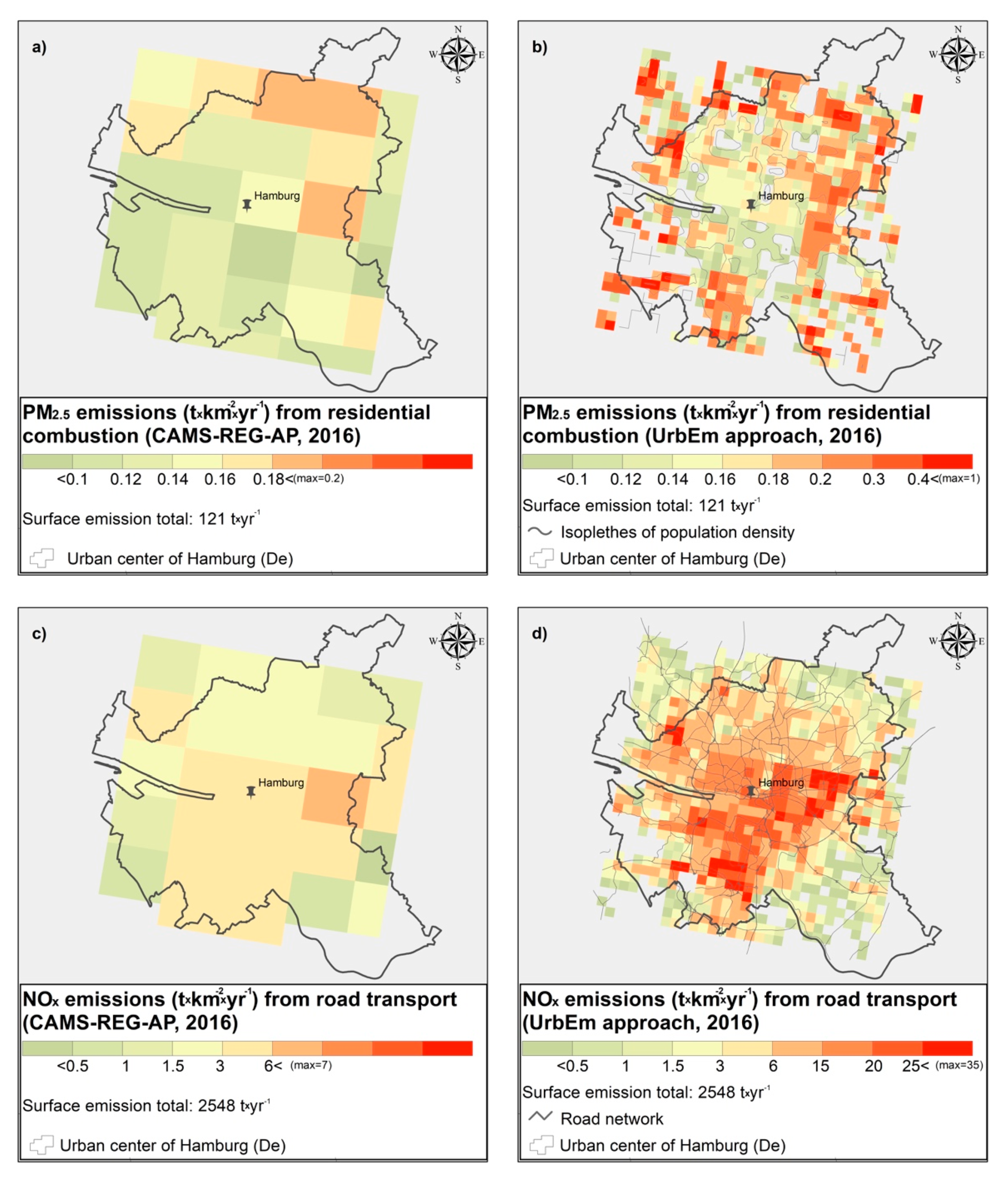
3.1. Comparison of Air Pollution Emissions

In order to identify the spatial differences and optimization of the European emission inventories (here CAMS datasets) when downscaled at the local level, representative species of selected source sectors are mapped for two scenarios: through the UrbEm approach (UrbEm scenario) and through a uniform spatial disaggregation of the original annual emission rates (CAMS no proxy approach or no-proxy scenario). The two cities that act as demonstrators of the value of the current development are Hamburg (Germany) and Athens (Greece) (Figure 5). Emission totals for the urban domains are compared to official reports or publications (Section 3.1.1 and Section 3.1.2), and differences in the spatial distribution provided by the two approaches are discussed. It should be noted that the two sets of gridded emission rates serve also as inputs to the city-scale model applications for both cities (Section 3.2).

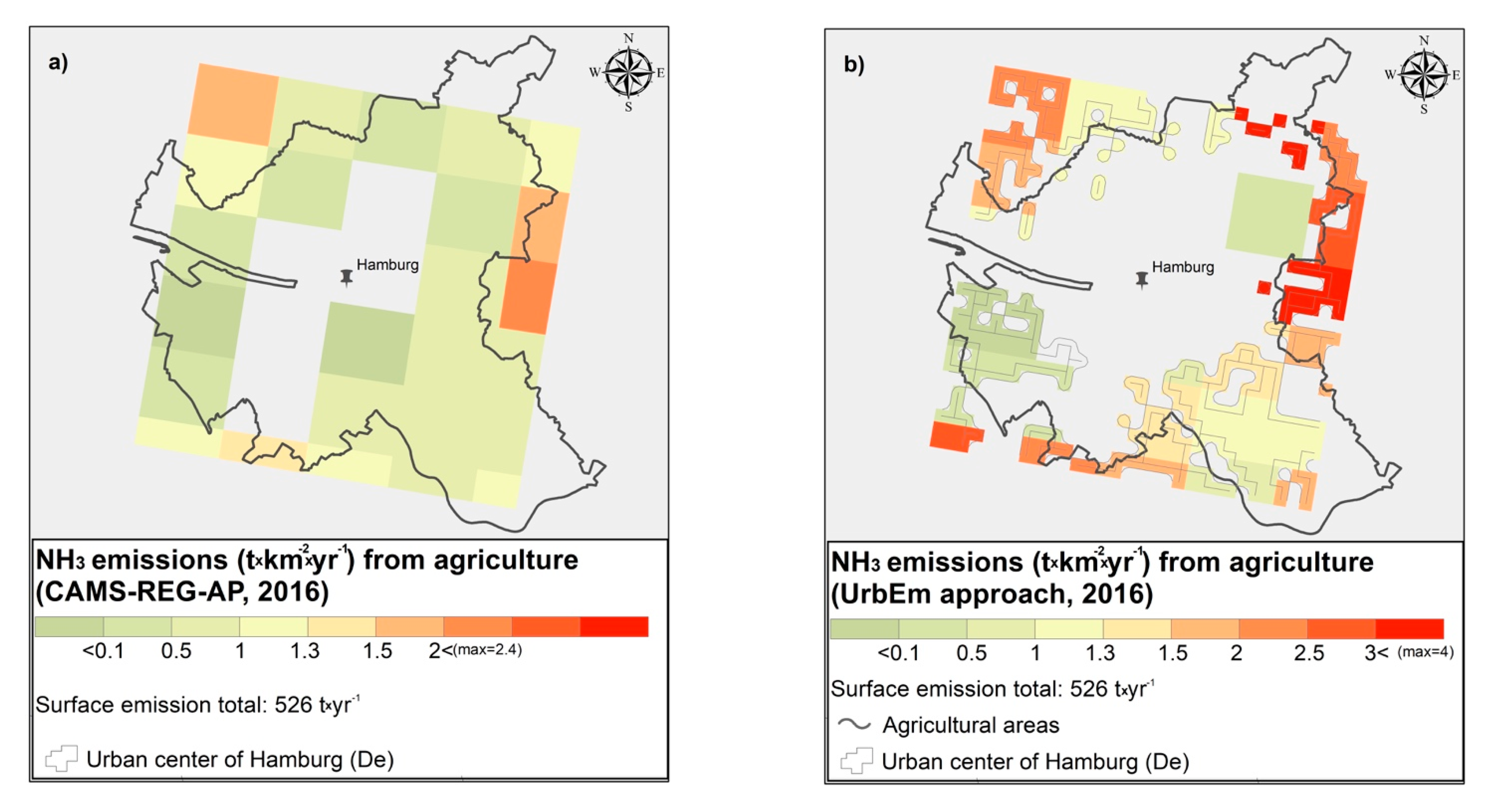
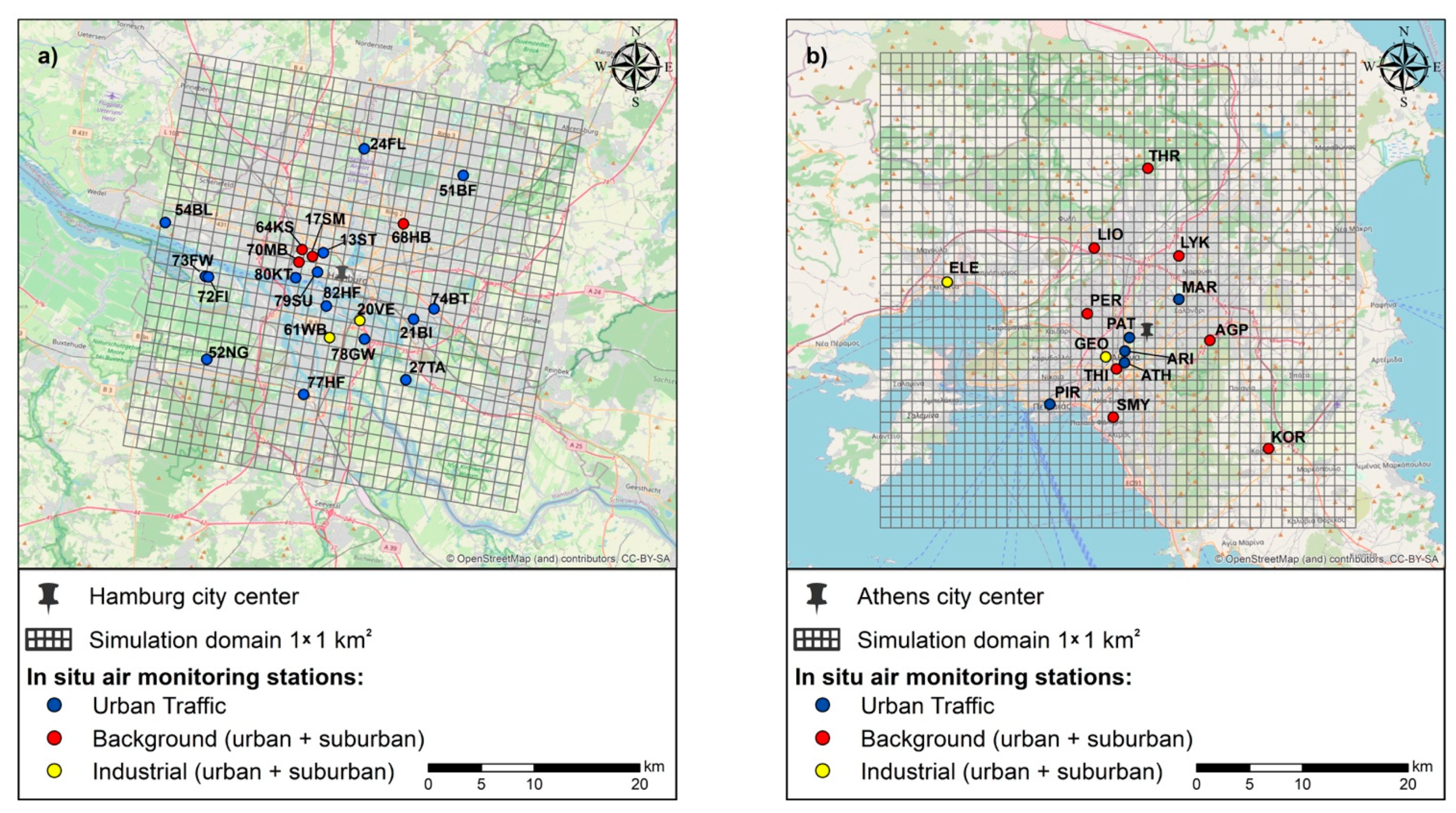
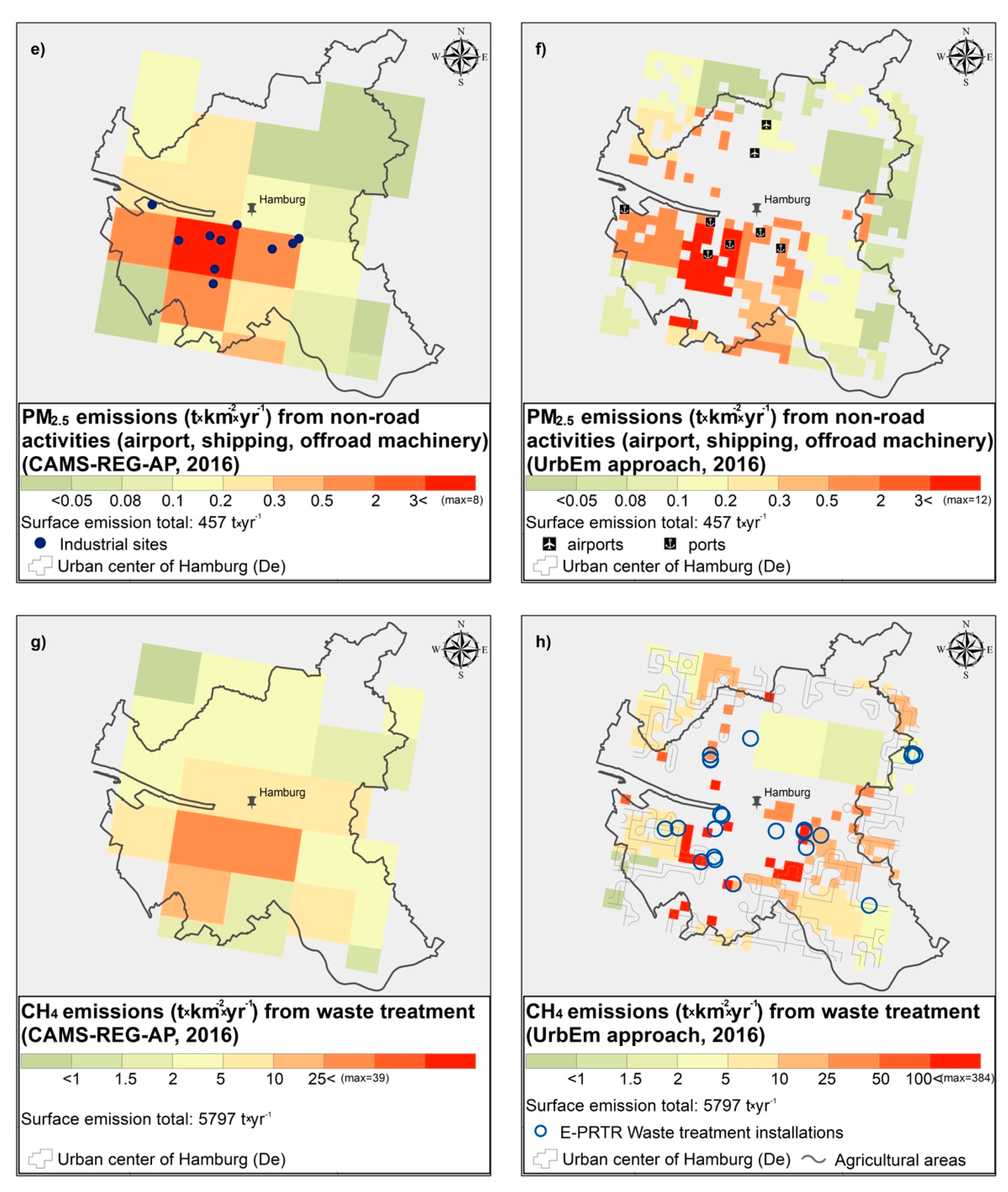
3.1.1. The Hamburg Demonstrator

The Free and Hanseatic City of Hamburg (Figure 5a) is a federal state and the second-largest city in Germany with a population of over 1.8 million people. Hamburg lies at the River Elbe, which connects the city with the 110 km distant North Sea, making it the gateway to Europe’s third largest international port. According to the municipality of Hamburg, road traffic and shipping have been contributing with 35% and 38% to total NO_X emissions as well as 30% and 17% to total PM₁₀ emissions in 2012, making the transportation sector the largest emission source for NO_X and PM₁₀ [33]. Although overall air quality in Hamburg has improved in recent decades, there are still exceedances of NO₂ limit values as defined by air quality standards of the European Union. In Hamburg, there is a well-established air quality monitoring network (Hamburger Luftmessnetz, HaLM, http://www.luft.hamburg.de, accessed: 23 October 2021) continuously measuring air pollutants such as NO₂, NO, PM₁₀, PM_2.5, SO₂, CO, O₃, and a several heavy metals. It consists of about 15 measurement stations at traffic, industry, and urban background sites. Since PM₁₀ and NO₂ limit values were exceeded in recent years, especially at traffic stations, the municipality of Hamburg established its first Clean Air Plan to tackle these exceedances with a variety of actions in 2004 [34]. These plans have been updated in 2012 and 2016.

For Hamburg, there exists a detailed inventory on point sources as derived through mandatory emission reporting under the Federal Emission Control Act, as well as a bottom–up line sources emission inventory which was created and updated for air quality plans in Hamburg 2012 and 2016 [33,35]. The point sources are available every four years (e.g., 2012, 2016), do not cover all criteria pollutants, and are measured, calculated, or estimated. The line sources are based on traffic density and flow data from measurements in combination with traffic-flow modeling and emission factors by HBEFA for the year 2011 [36]. Additionally, there exist scenario calculations for other years. When it comes to other sources such as agriculture, residential heating, airports, etc., emission totals are derived from different sources and gathered in the air quality plan, but no spatial distribution of such emissions is provided. The German Environment Agency offers tools [37] for spatial distribution of nationally reported emissions from different sectors with resolutions of up to 1 km based on different proxies. Nevertheless, such emissions are only available for specific years upon request and are spatially limited to the city’s boundaries. Thus, the suitability of such emissions for urban-scale CTMs is very limited.

As a first step to evaluate the UrbEm approach, we compared reported emission totals as given in the Clean Air Plans for 2012 and 2016 with emissions as created with the UrbEm approach from CAMS-REG inventory. Therefore, we applied an urban domain definition for Hamburg in the UrbEm approach, which has an extent of 30 × 30 km² with a resolution of 1 km and covers most of the Hamburg metropolitan area but also some surrounding areas (Figure 5a). In the Hamburg air quality plan for 2016, there are only NO_X emissions reported for the sectors road traffic, industry (incl. energy generation), residential heating, shipping, aviation, railroad, and off-road. When compared to the reported residential heating emissions, the CAMS-REG emissions for the same extent show 25% less NO_X emissions; for shipping, aviation, railroad, and off-road, which can be categorized as the SNAP8 sector, there are 40% less NO_X emissions calculated with UrbEm. In terms of shipping, this high underestimation is mainly due to ship emissions being roughly estimated in the municipality report, while shipping emissions in the CAMS-REG are based on model calculations taking into account AIS-based ship movements [38]. The comparison of road traffic shows slightly higher emissions totals (2%) when applying the UrbEm approach including a factor of 3 to increase road traffic emissions in the urban center. The comparison of reported emissions from industry and energy production with the sum of SNAP sectors 1, 3, and 4 shows 9% higher emissions with the UrbEm approach.

The second step to compare the UrbEm approach with Hamburg as a demonstrator is the analysis of spatial emission distribution. As indicated above, besides detailed information on reported high emitting industrial point sources and emissions from the main road network, there exist no official emissions inventory with spatially distributed emissions.

For the residential combustion sector, CAMS emissions are re-distributed with spatial proxies based on population density. Using these proxies leads to a distribution of emissions that matches the major residential areas in the north of the city center (PM_2.5 is showed exemplary in Figure 6a,b). In addition, the ratio of relatively high to relatively low emission areas in the population density proxy approach is similar to the respective ratio in CAMS. For the road network sector, CAMS emissions are redistributed with line proxies based on OSM. Thus, the distribution accurately matches the road network of the city of Hamburg (e.g., NO_X displayed in Figure 6c,d). Moreover, first comparisons of road traffic emissions derived with the UrbEm approach to more recent bottom–up modeled emissions based on HBEFA4.1 emission factors [36] and data on traffic density given by the Hamburg municipality revealed good agreement in terms of NO_x and PM emission totals and their spatial distribution, with slight underestimations toward the city center. Spatial proxies for the non-road transport, waste, and agricultural sector are derived from the Corine Land Cover 2018 dataset [24]. For the non-road transport sector (Figure 6e,f), the high emission areas are now concentrated on the corresponding sources of emissions—Hamburg port and airport Hamburg Fuhlsbüttel. Especially in terms of emissions from port activities by shipping, the spatial distribution is improved compared to the coarser CAMS emissions. Since there are residential areas close to the port areas, this turns out to be a crucial improvement for air quality management assessments. It needs to be mentioned that the Airbus airport is not represented by the CLC proxies, because the Airbus facility is considered an industrial area instead of an airport, although it is frequented by air transport. Redistributed CAMS emissions in the waste sector (Figure 6g,h) are concentrated on high-emission areas in the south of the city center and spatially match waste treatment plants and recycling facilities. Hamburg is surrounded by agriculturally dominated areas. The redistributed emissions in the agriculture sector sufficiently represent the peak emission areas in the southwest of the city (“Altes Land’’) and in the north and east of the city (Appendix C). In total, the applied spatial proxies in the UrbEm approach to downscale regional CAMS emissions in the Hamburg area match the most important features, which are necessary to represent the spatial distribution of emissions in air quality modeling and management.

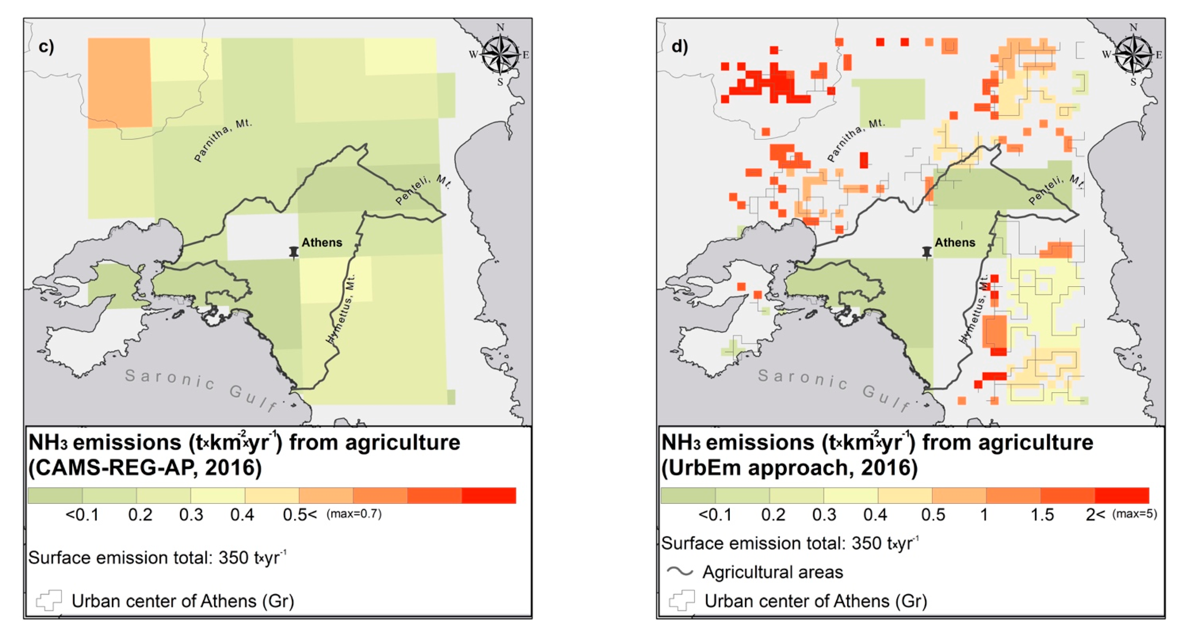
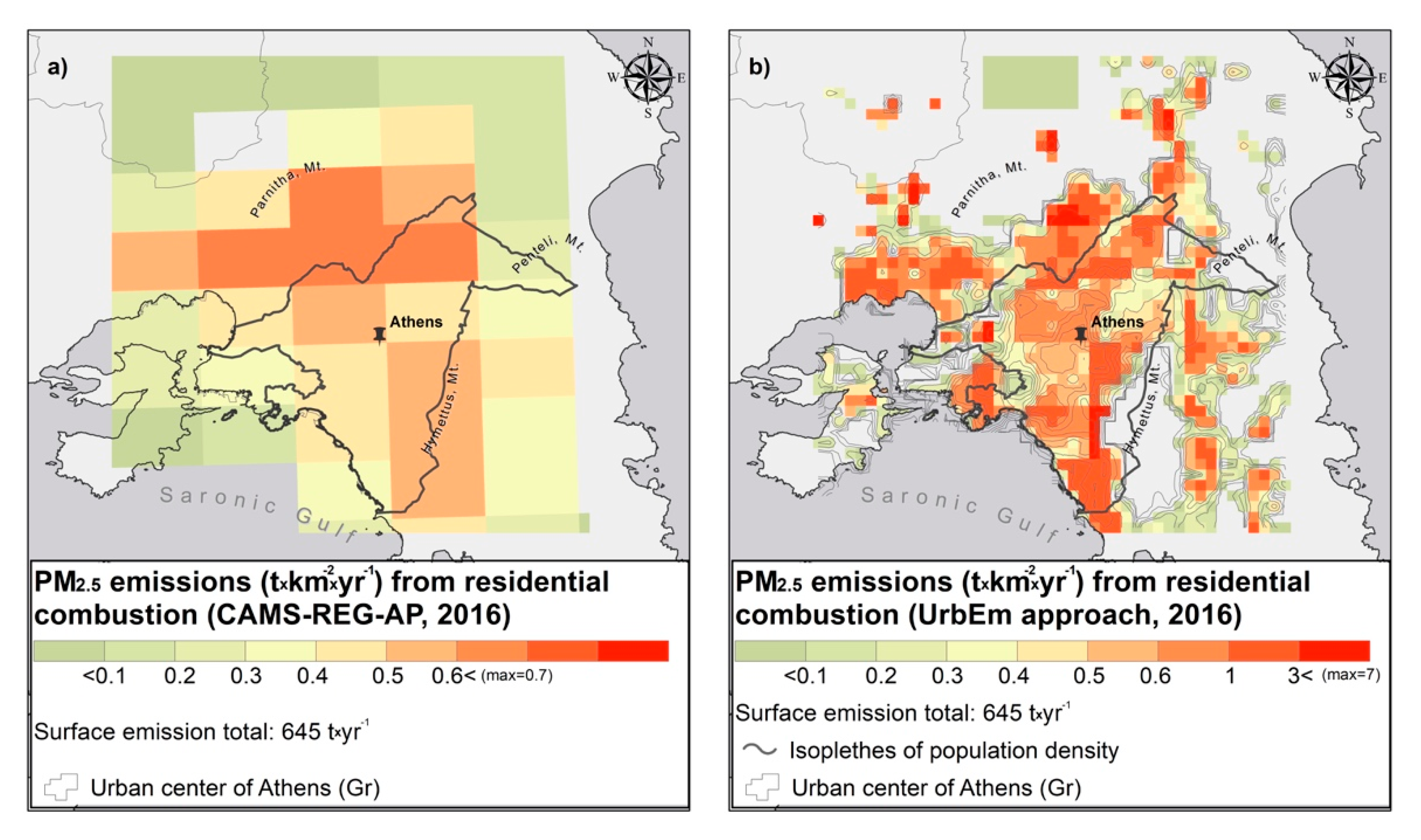
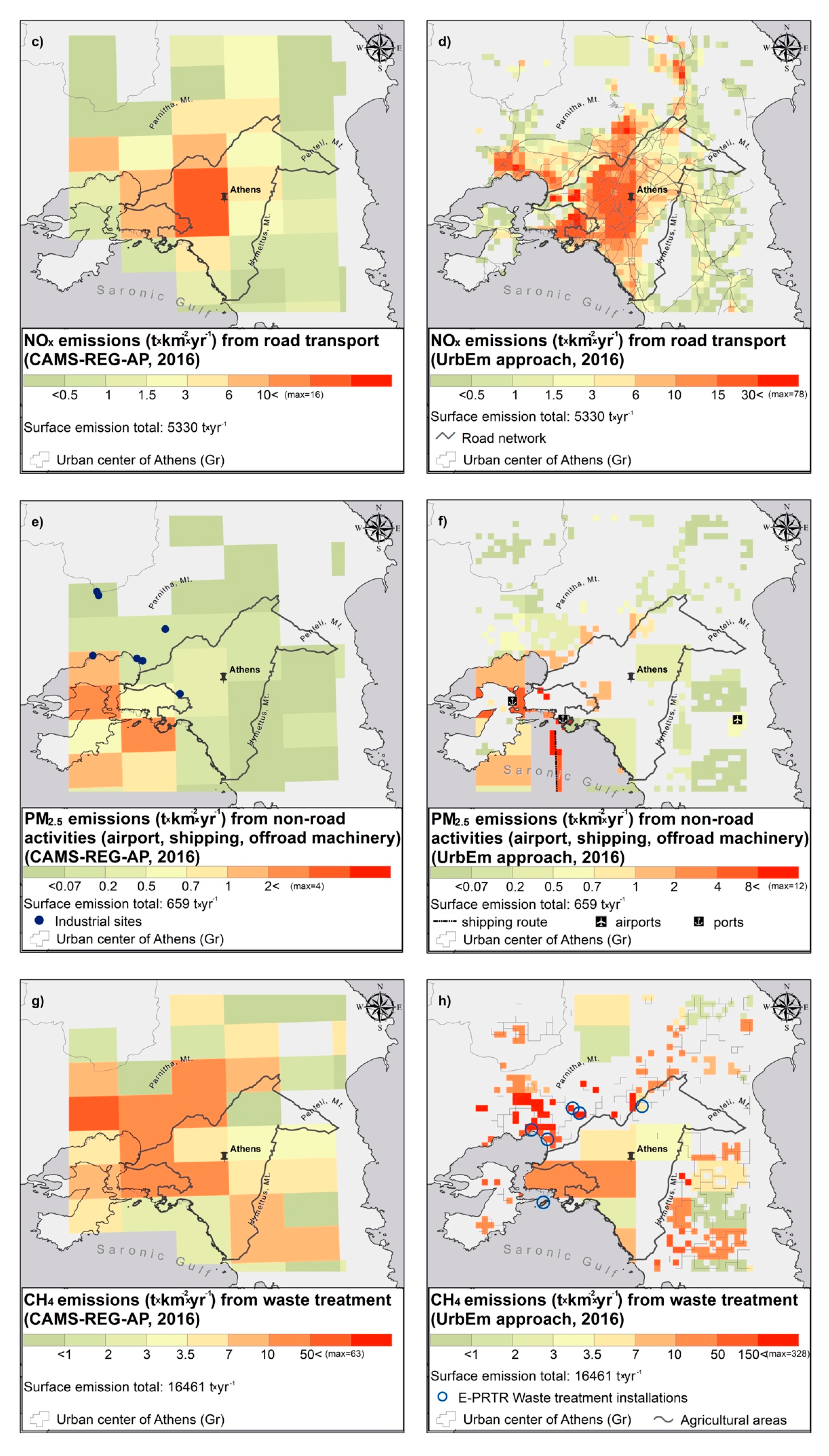
3.1.2. The Athens Demonstrator

Athens (Greece) is one of the biggest urban agglomerations in the eastern Mediterranean, which is bound by medium-altitude mountains and by the Saronic Gulf to the south–southwest [39,40]. The Athens basin (450 km²) concentrates the majority of the population (more than 3 million) and economic activity of the Greater Area of Athens, which combined with intense primary emissions, complex topography, and meteorology leads to high levels of atmospheric pollutants [41,42,43].

A large number (over 2.8 million) of vehicles are circulating in the area, of which approximately 90% are gasoline-powered private cars [42]. Road transport is responsible for a substantial part of not only NO_X but also PM_2.5 emissions [39,44]. The persistent economic recession has led to a shift in the fuel used for residential heating from fossil fuel toward biofuels, primarily wood, which in turn has caused pronounced wintertime air quality events, especially regarding particle pollutants [41,45]. The major non-traffic, non-heating activity affecting the Athens basin is shipping at and around the port of Piraeus, which is the largest passenger port in Europe and the second-busiest container port in the Mediterranean. Industrial activity inside the Athens basin is limited [39,42].

Over the last decades, NO₂ and PM levels have gradually decreased, although frequent smog events (and violations of the limit values) occur, mostly during wintertime [41,43,46,47]. The air quality of Athens is regularly monitored by the National Monitoring Network (Figure 4b). In situ measurements are also routinely conducted at the Thissio (THI) Air Monitoring Station (37.97326° N, 23.71836° E, 105 m a.s.l, 4 m a.g.l.) of the National Observatory of Athens (NOA), which is considered representative of background conditions in the central Athens basin [48,49,50].

Athens lacks official gridded and total emission data to compare with the UrbEm result for Athens. To this end, the scientific literature was explored, while applying the algorithm for 2016, for an extent of 45 × 45 km² (1 × 1 km² cell size) centered at the urban center (official definition by JRC), including both the neighborhood industrial area (at the west) and the national airport (at the southeast). The current comparative findings add value to the evaluation of the spatial allocation of the official national totals at the urban level, which are performed uniformly over Europe by the CAMS methodology [18]. To the best of our knowledge, such comparisons are not yet published for any urban area of the Eastern Mediterranean.

A literature search revealed several national and/or local gridded emission inventories [51,52,53,54,55,56]. Despite the divergence in the year of reference (from 1990 to 2010), surface coverage (e.g., Attica prefecture, Greater Athens Area, Athens basin, urban compound/area), and pollutants (NO_X, PM_2.5, PM₁₀, NMVOC, CO) of these emission datasets, the total CAMS NO_X emitted from the urban center of Athens for 2016 (27,774 t yr⁻¹) is consistent with the respective total for 1990 (44,200 t yr⁻¹, according to Zachariadis et al. [56]) decreased by the officially reported factor (approximately 0.4) from 1990 to 2016 for Greece reports (EIONET Central Data Repository, https://www.eionet.europa.eu, accessed: 23 October 2021). Similar consistency is also found for PM_2.5 between 1998 (4888 t yr⁻¹, according to Economopoulou and Economopoulos [51] and 2016 (2315 t yr⁻¹), using the officially reported decrease factor of 0.5. The industrial sector CAMS NO_X emission totals for Athens (21,139 t yr⁻¹) are similar to those reported by Markakis et al. [52] for 2003 (22,400 t yr⁻¹). For road transport emissions, the comparison among datasets is more challenging. CAMS urban center totals (using the EIONET conversion factors from 1990 to 2016) are significantly lower than all published totals emitted from Athens. The modeling analysis performed by Kuik et al., 2018 [28], suggests that traffic emissions by CAMS are strongly underestimated, which is in alignment with the aforementioned discrepancy and is partly attributed to the inadequate representation of traffic congestion. A distinct difference among the spatial distribution of emission totals stems from the expanded urban area for 2016 when compared to all previously published maps.

Focusing on the performance of the spatial disaggregation approach, we have developed comparative maps of the regional CAMS, and the local scale UrbEm emissions from Athens sources are given in Figure 7. Some findings apply to all types of sources and are due to the complex topography of Athens. For example, residential combustion emissions from coarse resolution grid cells (Figure 7a) extend beyond the coastline, whereas the use of population density as a high-resolution proxy to redistribute this sector eliminates this error (Figure 7b). Along the same line, the algorithm attributes all emissions from anthropogenic activities around mountainous areas at the downhill urbanized cells (e.g., road transport; Figure 7c,d). As evident through the mass totals (given at the bottom of each plot in Figure 7) and the spatial distribution of emissions within each coarse cell, although mass is conserved, the range of emission values is amplified by a factor of ca. 5 (road transport and waste treatment) or 10 (residential heating and non-road activities) for the high-resolution mapping. The pronounced gradient of UrbEm spatial fields is definitely an improvement stemming from the appropriate and high-resolution spatial proxies, which are used to allocate CAMS gridded emissions. The proxies are contemporary and frequently updated to ensure the consistency with the actual urban landscape during the period of study. The efficiency of this optimization is quantified in the next section.

Examining each source sector separately, the UrbEm approach depicts spatial features of the air pollution emissions from residential combustion sources that coarse mapping fails to capture (Figure 7a,b). In particular, emissions are allocated at the inhabited areas in and around the urban center, with maximum values in the northern suburbs and in the mountainous residential areas. Most of the particulate matter emitted from residential combustion activities is known to originate from biomass (wood) burning, according to CAMS data for Greece. The latter (in particular TNO-MACC II [57]) has been proven reasonable for Athens during the economic crisis [48]. Therefore, the specific high-resolution dataset is expected to accurately represent residential wood burning emissions in Athens from 2009 to the present.

The biggest asset of the developed tool lies beyond the hybrid mechanism to produce the spatially disaggregated road transport emissions, either in fine (1 × 1 km²) cells or attributed to the contemporary road network of the studied city. As expected, the spatial allocation of vehicle emissions through CAMS (Figure 7c) is performed with consistency to the density of the Athens road network (Figure 7d). The finer disaggregation applied through UrbEm reveals spatial gradients and emission maxima from roads in more detail and accuracy. The optimization of air pollution from road transport is realized when the emitted masses are ascribed to lines and then combined with air quality models that incorporate urban canyon processes (see Section 3.2).

Waste treatment emissions are known as more localized than how they are represented by CAMS (Figure 6e). With the usage of the locations of waste treatment installations, mass allocations are performed in higher accuracy (Figure 7f). The open burning of waste has an increased positioning uncertainty, as it can potentially occur on any agricultural surface.

CAMS data representing emissions from non-road activities (Figure 7g) are greatly improved by allocating airport and shipping emissions at their actual land and sea surfaces (Figure 7h). Shipping is indeed found as a pronounced source of air pollution, which is consistent with what is stated above for Athens. With respect to non-road machinery, its allocation follows the same restrictions mentioned for open waste fires.

3.2. Verification through Air Pollution Predictions

The evaluation of the developed approach (UrbEm) to arrive at urban, high-resolution emission inventories is performed through their implementation in atmospheric numerical simulations. In particular, AQ predictions for Hamburg are performed for 2016 and compared with observations from 13 and five stations measuring NO₂ and PM_2.5, respectively (Figure 4a). For Athens, a heavily polluted month (December 2018) is used to demonstrate the value of high resolution (including linear road) emissions for a city that faces complex challenges, as described in Section 3.1.2. NO₂ and PM_2.5 observations made by the National Monitoring Network (Figure 4b) and at the supersite at Thissio [50] are compared with the respective predictions. In both demonstrators, the urban stations are categorized and grouped as traffic, background, and industrial.

In order to quantify the assets of the UrbEm approach discussed in Section 3.1, namely the use of high-resolution spatial proxies for area emission distribution, plus the allocation of road transport emissions in line sources, the CAMS (no proxy) and UrbEm emission datasets already discussed in Section 3.1 stand as the core of the two emission scenarios applied in both demonstrator cities (CAMS no proxy and UrbEm scenario, respectively). Based on the already mentioned findings of Kuik et al. (2018) [28], the proposed multiplication factor of 3 is applied in the emissions by road transport. As this was found to remediate underestimations in regional emission inventories (as well as other possible sources of model biases), it is also applied in the CAMS no-proxy scenario. Such a consistency keeps comparisons among scenarios linked to their spatial divergence.

Hourly emission rates are calculated by using the monthly, weekly, and diurnal profiles indicated through Bieser et al. (2011) [58] for each source sector. The monthly profiles for road transport in Athens are adjusted according to national data [59]. Daily and hourly profiles for residential heating are based on air pollution measurements in Athens [48]. Additionally, area emissions of residential heating are generated with dependence on the daily average temperature in Hamburg and Athens. Lastly, the split of NO_X (CAMS output) to NO and NO₂ emissions (EPISODE-CityChem inputs) is 95:5 for area and point and 70:30 for line emissions.

Emission databases correspond to reference years. In order to provide high-resolution emissions for any year of interest, the official, national reports (EIONET Central Data Repository, https://www.eionet.europa.eu) of total emissions are compared. The extracted multiplication factors per source and pollutant are applied and convert emissions from the year of reference to the year of interest.

3.2.1. Chemistry Transport Model Setup

EPISODE-CityChem is a Chemistry Transport Model to enable chemistry/transport simulations of reactive pollutants on the city scale. In particular, the horizontal spatial resolution of simulations is 1 km with an embedded regular receptor grid (100 m × 100 m), which hosts Gaussian line and point source dispersion and local photochemistry [22]. More details on the features of the model and its configuration and setup for the current study can be found in Appendix B.

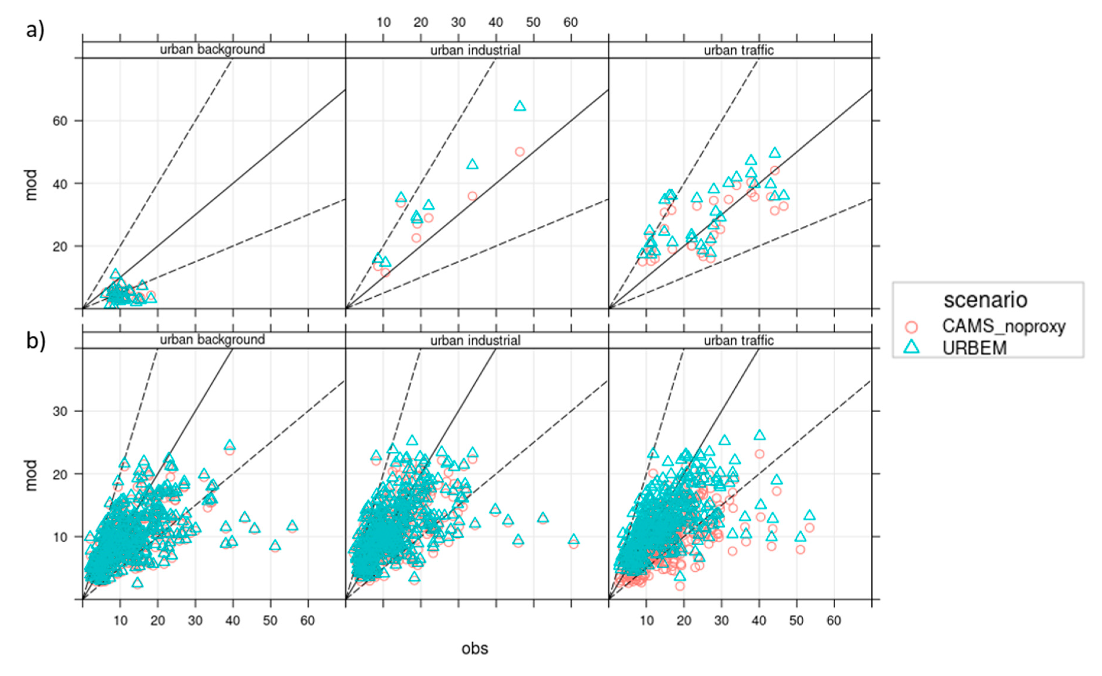
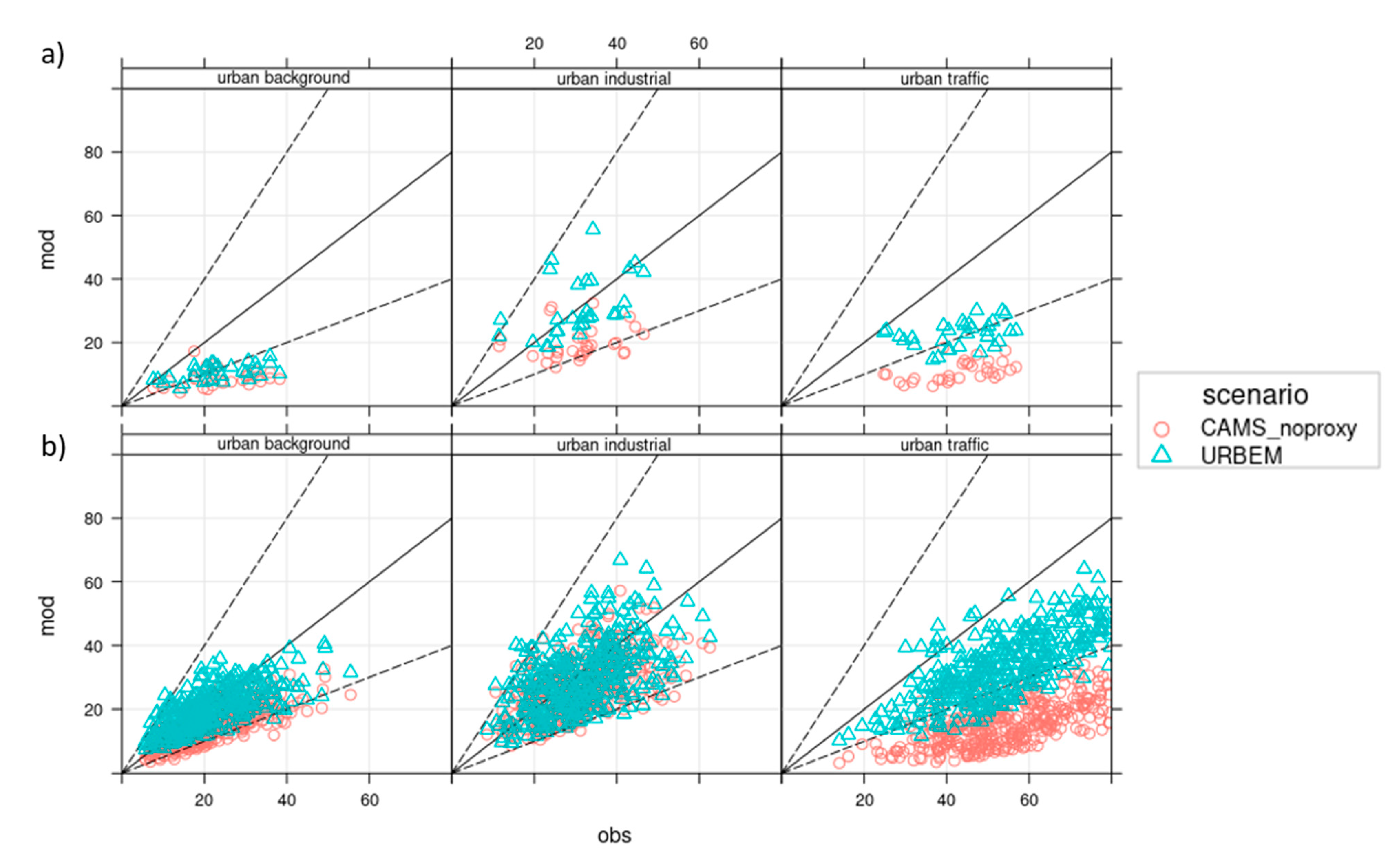
3.2.2. Comparison of Predictions and Observations

The comparison with available observations (sites of which are shown on Figure 4) support the efficiency of the UrbEm approach, especially for NO_X. In particular, the EPISODE-CityChem model is found to underestimate observations (Appendix C) in both cities, but the intercomparison of the average mean biases from CAMS no proxy to UrbEm shows a significant reduction of this underestimation by more than 100% in most cases. Indeed, NO₂ predictions from these two model runs have been compared, and their difference is found statistically significant at the 95% confidence level (p < 0.05) for all stations in both cities. The temporal correlation (r) among measurements and observations is significantly improved when replacing the CAMS no proxy and the UrbEm approach. As expected for urban environments, the deviation of observations from their mean value is elevated, which cannot be represented when emissions are coarsely allocated to their sources (CAMS no-proxy scenario). In contrast, UrbEm enables the depiction of a greater dispersion of air pollution around the mean urban values, which is reflected through the higher standard deviation found, better matching the real case in both cities. In addition, the fraction of modeled values within a factor of two of the observed values is in most stations above 50%, reaching 75% for PM_2.5, when the UrbEm scenario is considered. The greatest improvement of model performance occurs for NO₂ over the industrial and traffic urban areas of Athens as well as for Hamburg (Figure 8). This is attributed to the strong spatial variation of urban land types, and thus of emission sources, when combined with elevated anthropogenic emissions during wintertime, the short lifetime, and strong gradients of NO₂. This combination necessitates the right spatial allocation of urban emissions, namely at the road network and the industrial sites generating much stronger gradients when compared with a coarser resolution grid.

In order to proceed to a targeted inter-comparison between the two model scenarios/disaggregation approaches, Figure 8 (and Appendix C) presents the scatter plots to show the deviation of model predictions for mean daily NO₂ (and PM_2.5) from the observed values (markers upon the solid 1:1 line) up to a factor of two (markers inside the dashed 1:2, 2:1 lines) and further (markers outside the dashed lines). An overall statement is the comparative advantage of the UrbEm approach, shifting the cloud of observation–prediction pairs toward the 1:1 line, which is striking for NO₂. This performance is more apparent in emission hotspots (traffic or industrial areas) and is explained by their more accurate spatial representation by the UrbEm approach. Especially for the urban traffic sites, the significance of the line representation of road transport emissions is revealed through the distinct position of the CAMS no proxy outside the dashed lines. Through high-resolution emission allocation, mass rates from their actual hotspots (e.g., roads, industrial sites, residences) are increased; thus, concentration underestimations over and downwind primary emissions are decreased.

The effects of the UrbEm approach on PM_2.5 model performance are less pronounced (Appendix C). This is expected over and downwind urban traffic areas, because traffic has a smaller footprint on PM_2.5 and hence on its spatial disaggregation. More broadly and independent of pollution sources, PM_2.5 shows less spatial variability due to its governing atmospheric processes, including the role of secondary inorganic and organic formation of atmospheric aerosols. Overall, the applied downscaling is especially valuable for short-lived species, but in some cases, improvements can be seen also for PM_2.5. It is worth mentioning that these improvements are important, given the statistical comparison performed among the two model scenarios, which found their difference significant at the 95% confidence level (p < 0.05) for all stations in both cities.

Focusing on the air pollution mapping over the complex area of Athens during a highly polluted winter month, it seems that the spatial optimization of coarse emissions contributes more than 30% and up to 70% to the modeled NO₂ concentrations over most of the urban area (Figure 9a) and the other polluted areas outside (e.g., the industrial area in the west and the national road toward the north). Indicatively, over the sites of model-measurement mean monthly inter-comparison (e.g., PIR, ELE, PER, LIO), the UrbEm approach improves model results by 30–50% when compared to the CAMS no-proxy scenario.

The contribution of UrbEm to the mean monthly PM_2.5 predictions (Figure 9b) based on CAMS emissions is lower (up to 30%) and occurs mainly outside the urban center, over the industrial areas and the northern residential suburbs. These maxima of UrbEm effects are related to the spatial optimization of industrial emissions and residential combustion, respectively. From the four measuring sites of PM_2.5, only the predictions at the urban traffic site at the port (PIR) seem to differentiate around 20%, with the UrbEm approach being consistent with the mean monthly observations.

Figure 9c,d illustrate the differences between the CAMS no proxy and UrbEm for both NO₂ and PM_2.5 concentrations in Hamburg. Especially for NO₂, the linear structures of the road network become more distinct in the UrbEm approach. In general, the UrbEm approach allows a wider distribution of concentrations in the city domain. For both NO₂ and PM_2.5, it is expectable that the concentrations peaks are in the city center and the port area, which is additionally a hotspot for industrial activities. For further discussion of air pollutant concentration for Hamburg in 2016 as derived from emissions downscaled with an early version of the UrbEm, we refer to Ramacher and Karl (2020) [29].

4. Discussion

The comparison of downscaled regional CAMS-REG emissions (≈6 × 6 km² grid cells) with the introduced UrbEm approach to the same emissions that were mapped to our high-resolution grid without the use of any spatial redistribution proxies showed substantial changes in the fields of emissions in Hamburg and Athens. The city-specific exploration of local features, such as waste and recycling facilities, road networks, industrial and agricultural areas, as well as the locations of ports and shipping lanes guided and optimized the spatial distribution of connected emissions through the use of the appropriate, detailed spatial proxies in the frame of the UrbEm approach. The approach is of utmost importance for modeling air quality for coastal cities, as it ensures zero emissions from the sea surfaces that are adjacent to land-oriented emissions and vice versa. Despite the claim of the UrbEm approach to be generally applicable in European cities, there are some remaining imprecisions in the spatial distribution, e.g., the consideration of all types of airports, independent of their use (e.g., public or military) or the specific location of point sources with high emissions that are not covered by the E-PRTR emission inventory because they are below the reporting thresholds. Thus, knowledge, if possible, on the local emission features, can optimize the outputs of the UrbEm approach, as well as reveal desired deviations from the horizontal CAMS methodology at the domains/cities under study.

Considering the treatment of road traffic emissions, the UrbEm approach allows for distributions of emissions to any city’s road network by using OSM data. Evidently, that improves the distribution of road traffic emissions when compared to grid emissions. Thus, this feature is of high value for any detailed spatial analysis of urban air pollution, while it can be essential for urban-scale air quality models capable of handling road emissions from line instead of area sources. The coupling of UrbEm with Episode-CityChem for two city demonstrators showed an increased accuracy and a better representation of gradients in intra-urban air pollution predictions. According to a recent sensitivity study on the choice of the subgrid resolution in urban-scale air pollution modeling [60], the 100 m resolution (used here) has been found competent to represent near-road concentration estimates. Nevertheless, model underestimations at road traffic sites remain both in Hamburg and Athens, even though we applied the emission correction factor of 3 proposed by Kuik et al. (2018) [28] to all pollutants in both cities. A possible reason might be the ventilation effects and concentration agglomerations in street canyons or at junctions that might not be adequately represented in chemistry transport modeling. Another source of discrepancy could be the uniform application of the NO to NO₂ ratio, which was applied to split the NO_X input provided by CAMS. Additionally, occasional heavy traffic at intersections and traffic jams is not taken into account when conventional temporal emission profiles are applied. Similarly for the spatial dimension, the distribution of regional road traffic emissions to urban-scale road links as derived from OSM does not take into account city-specific traffic densities, congestion, or other spatial features that may be applied in bottom–up approaches. Lastly, a frequent source of model discrepancies is the non-accounted air pollution sources in emission inventories, such as the recirculation/resuspension of particulate matter due to vehicle movement [48,53].

The UrbEm approach does not claim to replace city-specific emission modeling efforts or bottom–up emission inventories. Nevertheless, the creation of bottom–up anthropogenic emissions is still a demanding and expensive task due to the necessary collection of city-specific data (e.g., road-specific vehicle densities, fleet compositions) and their compilation toward emission rates per source and pollutant. In addition, most of the detailed city-specific emission inventories are available for specific years and/or upon request; these are spatially aggregated or their disaggregation is frequently in cells above 2 km spatial resolution, road (and occasionally industrial) emissions are attributed to cells (instead of lines or points), and it is limited to municipal boundaries or prescribed domains. In cases, specific sources and/or pollutants could be missing from existing local inventories. In addition, for big cities, such as Athens and Hamburg, there are lots of high-resolution data for adequate urban air quality modeling temporally and spatially aggregated or missing. Lastly, the scope of city-scale inventories may be different from typical national or European-wide inventories, which makes it difficult to nest the city-scale inventory into a wider regional inventory [61].

Therefore, the UrbEm approach enables urban air quality planners and modelers that lack resources and city-specific information to initiate efforts in air quality management. For cities such as Athens, with a complex terrain and official emissions at the national level, the UrbEm approach to downscale open regional emissions adds value to air quality management efforts by using the detailed spatial proxies in downscaling. Taking into account that the spatial data that underlie the applied proxies in the UrbEm approach are frequently updated and/or become more detailed, we expect the spatial representativeness of emissions downscaled with UrbEm to enhance. Indicatively, once the building height data by CLMS (https://land.copernicus.eu/local/urban-atlas/building-height-2012, accessed: 23 October 2021) become available for all European cities (rather than solely capitals), its incorporation to our approach will certainly optimize the spatial allocation of residential heating emissions.

Through this work, it is shown that the high-resolution emission allocation with UrbEm improved the performance of modeled values from a state-of-the-art city-scale CTM. Such an approach provided also flexibility in the selection of the region, resolution, and period of interest for AQ modeling. Lastly, comparative modeling studies among several European cities is feasible and concrete when using gridded emission data produced by the same methodology and tool, based on a common European database, thus aligning with the call from the European Commission’s recent Air Quality—Fitness Check of the AAQ Directives for further harmonizing modeling activities across the EU [62].

Overall, the investment upon existing knowledge and data hosted on reliable programs/platforms such as Copernicus/CAMS is an approach to overcome the lack of bottom–up high-resolution emission inventories for certain cities, or it can be an equivalent alternative to pre-existing local emission data. Whichever the case, such exploitation and development can certainly act as feedback toward the continuous improvement and optimization of the provided services.

5. Conclusions

The use of regional emission inventories can be challenging for urban-scale AQ applications and air quality management in cities. Nevertheless, their exploitation through disaggregation by utilizing spatial proxies, available on a European or global scale, is a credible solution for European cities that lack bottom–up emission inventories. To this end, we developed the UrbEm approach, which enables in a modular manner the downscaling of gridded regional emissions with specific spatial proxies based on a variety of open access, robust, sustainable, and frequently updated sources. The presented approach can be applied to any urban area in Europe and provides methodological homogeneity between different cities.

Prioritizing applicability and homogeneity, the developed approach avoids any dependence on occasional, local, high-resolution data, without excluding this option once such data (e.g., variable traffic volumes for specific road segments) are available for cities or periods of interest. Nevertheless, the method invests upon well-established European emission inventories (here CAMS-REG), which already have incorporated pollutant- and source-specific data (e.g., traffic densities, vehicle and road types), for the spatial disaggregation of national emission totals. All data that support the high-resolution spatial proxies used are being quality controlled and assured (see more on Appendix A), while the limitations relevant to CAMS-REG or any traditional top–down emission inventory are expected unless near real-time emission data were ideally available and used.

To demonstrate the general applicability and performance of the developed method and tool, we compared the spatial distribution of uniformly disaggregated regional emissions with emissions downscaled with the UrbEm approach for the differing cities of Athens and Hamburg. The representation of local features in general and of emission hotspots in particular was largely improved. We further applied the two emission inventories in a state-of-the-art urban-scale Chemistry Transport Model and compared the results against measurements. Urban-scale air pollutant concentrations based on the UrbEm approach show improved agreement, especially for NO₂ and measurement sites close to road traffic.

The UrbEm downscaling approach is completely free of cost and open source, which is accompanied with an efficient, fully automated, and intuitive tool (https://github.com/martinottopaul/UrbEm, accessed: 23 October 2021) that enables users to create high-resolution urban emissions from point, line, and area sources. We are confident that UrbEm fully covers the emission inventory prerequisite for all urban air quality modeling and management efforts and serves as a starting point for such efforts in cities across Europe.

While the work described here establishes UrbEm, we envision a continuous improvement of the methodology regarding its technical components such as the integration of improved proxies. Beyond the paradigm of the building height data by CLMS discussed already, the Automatic Identification System (AIS) data used for shipping emissions is such a candidate. The latter was exploited under the uEMEP implementation [60], which is a similar undertaking to ours and with whom we will pursue technical exchange regarding the use of proxies not currently handled by them. Moreover, comparisons between the two methodologies and with other bottom–up implementations in European cities would deliver a clear insight on the balance between overall resources required and efficiency across Europe. Relevant to this, comparative applications of atmospheric numerical models using UrbEm and bottom–up local inventories when and where available would further build the proof of efficiency of the method as well as reveal deficiencies to alleviate. Lastly, we plan to expand the automization of the whole workflow, minimize the need for location-specific refinements, and keep the process per city temporally efficient. A valuable addition would be the integration of the newly developed temporal profiles CAMS-TEMPO [63] toward producing hourly, instead of yearly, emission rates, based on spatially-variant temporal profiles.

On a more policy-related note, UrbEm aims at contributing to the current discussion on the Revision of Ambient Air Quality Directives [64] (https://ec.europa.eu/environment/air/quality/revision_of_the_aaq_directives.htm, accessed: 23 October 2021) and its ensuing policy implications. In particular, we aspire to support—Europe-wide—the mitigation of administrative burden of air quality management by offering such an agile tool, to increase the comprehensiveness of air quality assessments by providing a common staring point, and to bring out the underlying aspects of environmental inequalities present in the spatial distribution of emissions, concentrations, and exposure in urban locales while offering a credible solution for planning equitable measures.

References

1. United Nations. World Urbanization Prospects: The 2018 Revision: Online Edition. Available online: https://population.un.org/wup/Download/ (accessed on 23 October 2021).
2. Alberti, V.; Alonso Raposo, M.; Attardo, C.; Auteri, D.; Ribeiro Barranco, R.; Batista ES, F.; Benczur, P.; Bertoldi, P.; Bono, F.; Bussolari, I.; et al. The Future of Cities: Opportunities, Challanges and the Way Forward; Vandecasteele, I., Baranzelli, C., Siragusa, A., Aurambout, J.P., Eds.; Publications Office: Luxembourg, 2019; ISBN 9789276038474.
3. EEA. Air Quality in Europe: 2019 Report; Publications Office of the European Union: Luxembourg, 2019; ISBN 978-92-9480-088-6.
4. World Health Organization. WHO Global Air Quality Guidelines: Particulate Matter (PM2.5 and PM10), Ozone, Nitrogen Dioxide, Sulfur Dioxide and Carbon Monoxide; World Health Organization: Geneva, Switzerland, 2021. [Google Scholar]
5. Thunis, P.; Miranda, A.; Baldasano, J.M.; Blond, N.; Douros, J.; Graff, A.; Janssen, S.; Juda-Rezler, K.; Karvosenoja, N.; Maffeis, G.; et al. Overview of current regional and local scale air quality modelling practices: Assessment and planning tools in the EU. Environ. Sci. Policy 2016, 65, 13–21. [Google Scholar] [CrossRef]
6. Benavides, J.; Snyder, M.; Guevara, M.; Soret, A.; Pérez García-Pando, C.; Amato, F.; Querol, X.; Jorba, O. CALIOPE-Urban v1.0: Coupling R-LINE with a mesoscale air quality modelling system for urban air quality forecasts over Barcelona city (Spain). Geosci. Model Dev. 2019, 12, 2811–2835. [Google Scholar] [CrossRef] [Green Version]
7. Jerrett, M.; Arain, A.; Kanaroglou, P.; Beckerman, B.; Potoglou, D.; Sahsuvaroglu, T.; Morrison, J.; Giovis, C. A review and evaluation of intraurban air pollution exposure models. J. Expo. Anal. Environ. Epidemiol. 2005, 15, 185–204. [Google Scholar] [CrossRef]
8. Relvas, H.; Miranda, A.I. An urban air quality modeling system to support decision-making: Design and implementation. Air Qual. Atmos. Health 2018, 11, 815–824. [Google Scholar] [CrossRef]
9. Gulia, S.; Shiva Nagendra, S.M.; Khare, M.; Khanna, I. Urban air quality management-A review. Atmos. Pollut. Res. 2015, 6, 286–304. [Google Scholar] [CrossRef] [Green Version]
10. Matthias, V.; Arndt, J.A.; Aulinger, A.; Bieser, J.; van der Denier Gon, H.; Kranenburg, R.; Kuenen, J.; Neumann, D.; Pouliot, G.; Quante, M. Modeling emissions for three-dimensional atmospheric chemistry transport models. J. Air Waste Manag. Assoc. 2018, 68, 763–800. [Google Scholar] [CrossRef]
11. Trombetti, M.; Thunis, P.; Bessagnet, B.; Clappier, A.; Couvidat, F.; Guevara, M.; Kuenen, J.; López-Aparicio, S. Spatial inter-comparison of Top-down emission inventories in European urban areas. Atmos. Environ. 2018, 173, 142–156. [Google Scholar] [CrossRef]
12. Kadaverugu, R.; Sharma, A.; Matli, C.; Biniwale, R. High Resolution Urban Air Quality Modeling by Coupling CFD and Mesoscale Models: A Review. Asia-Pacific J. Atmos. Sci. 2019, 55, 539–556. [Google Scholar] [CrossRef]
13. Thunis, P.; Janssen, S.; Wesseling, J.; Belis, C.A.; Pirovano, G.; Tarrason, L.; Guevara, M.; Monteiro, A.; Clappier, A.; Pisoni, E.; et al. Recommendations Regarding Modelling Applications within the Scope of the Ambient Air Quality Directives: EUR29699 EN; Publications Office of the European Union: Luxembourg, 2019.
14. EEA. EMEP/EEA Air Pollutant Emission Inventory Guidebook 2016: EEA Report No 21/2016. Available online: https://www.eea.europa.eu/publications/emep-eea-guidebook-2016 (accessed on 15 February 2019).
15. Guevara, M.; Tena, C.; Porquet, M.; Jorba, O.; Pérez García-Pando, C. HERMESv3, a stand-alone multi-scale atmospheric emission modelling framework—Part 2: The bottom–up module. Geosci. Model Dev. 2020, 13, 873–903. [Google Scholar] [CrossRef] [Green Version]
16. European Environment Agency. Europe’s Urban Air Quality—Re-Assesing Implementation Challenges in Cities. Available online: https://www.eea.europa.eu/publications/europes-Urban-air-quality (accessed on 11 May 2020).
17. Kuenen, J.; Dellaert, S.; Visschedijk, A.; Jalkanen, J.-P.; Super, I.; van der Denier Gon, H. CAMS-REG-v4: A State-of-the-Art High-Resolution European Emission Inventory for Air Quality Modelling. Earth Syst. Sci. Data Discuss. (preprint), in review. 2021. [Google Scholar] [CrossRef]
18. Granier, C.; Darras, S.; Denier van der Gon, H.; Doubalova, J.; Elguindi, N.; Galle, B.; Gauss, M.; Guevara, M.; Jalkanen, J.-P.; Kuenen, J.; et al. The Copernicus Atmosphere Monitoring Service Global and Regional Emissions (April 2019 Version). 2019. Available online: https://atmosphere.copernicus.eu/sites/default/files/2019-06/cams_emissions_general_document_apr2019_v7.pdf (accessed on 6 February 2020).
19. Karl, M.; Ramacher, M.O.P. City-Scale Chemistry Transport Model EPISODE-CityChem. 2018. Available online: https://zenodo.org/record/4814060/#.YXO_CS-21pQ (accessed on 23 October 2021).
20. Karamchandani, P.; Lohman, K.; Seigneur, C. Using a sub-grid scale modeling approach to simulate the transport and fate of toxic air pollutants. Environ. Fluid Mech. 2009, 9, 59–71. [Google Scholar] [CrossRef]
21. Trombetti, M.; Pisoni, E.; Lavalle, C. Downscaling Methodology to Produce a High Resolution Gridded Emission Inventory to Support Local/City Level Air Quality Policies: EUR 28428 EN 10.2760/51058; Publications Office of the European Union: Luxembourg, 2017.
22. Karl, M.; Walker, S.-E.; Solberg, S.; Ramacher, M.O.P. The Eulerian urban dispersion model EPISODE—Part 2: Extensions to the source dispersion and photochemistry for EPISODE–CityChem v1.2 and its application to the city of Hamburg. Geosci. Model Dev. 2019, 12, 3357–3399. [Google Scholar] [CrossRef] [Green Version]
23. Florczyk, A.J.; Cobane, C.; Ehrlich, D.; Freire, S.; Kemper, T.; Maffeini, L.; Melchiorri, M.; Pesaresi, M.; Politis, P.; Schiavina, M.; et al. GHSL Data Package 2019: JRC Technical Report; EUR 29788 EN; Publications Office of the European Union: Luxembourg, 2019.
24. Copernicus Land Monitoring Service. Corine Land Cover. Available online: https://land.copernicus.eu/pan-european/corine-land-cover/clc2018 (accessed on 23 October 2021).
25. OpenStreetMap Contributors. 2018. Available online: https://planet.osm.org (accessed on 23 October 2021).
26. R Core Team. R: A Language and Environment for Statistical Computing; Vienna, Austria, 2019. Available online: https://www.R-project.org/ (accessed on 23 October 2021).
27. United States Central Intelligence Agency. Map of the world oceans. Available online: https://www.loc.gov/item/2013591571/ (accessed on 9 September 2021).
28. Kuik, F.; Kerschbaumer, A.; Lauer, A.; Lupascu, A.; von Schneidemesser, E.; Butler, T.M. Top–down quantification of NOx emissions from traffic in an urban area using a high-resolution regional atmospheric chemistry model. Atmos. Chem. Phys. 2018, 18, 8203–8225. [Google Scholar] [CrossRef] [Green Version]
29. Ramacher, M.O.P.; Karl, M. Integrating Modes of Transport in a Dynamic Modelling Approach to Evaluate Population Exposure to Ambient NO2 and PM2.5 Pollution in Urban Areas. Int. J. Environ. Res. Public Health 2020, 17, 2099. [Google Scholar] [CrossRef] [Green Version]
30. Florczyk, A.J.; Melchiorri, M.; Corbane, C.; Schiavina, M.; Maffeini, L.; Pesaresi, M.; Politis, P.; Sabo, F.; Freire, S.; Ehrlich, D.; et al. Description of the GHS Urban Centre Database: Public Release 2019, Version 1.0; Publications Office of the European Union: Luxembourg, 2019.
31. Ibarra-Espinosa, S.; Ynoue, R.; Sullivan, S.; Pebesma, E.; Andrade, M.d.F.; Osses, M. VEIN v0.2.2: An R package for bottom–up vehicular emissions inventories. Geosci. Model Dev. 2018, 11, 2209–2229. [Google Scholar] [CrossRef]
32. Seum, S.; Heinrichs, M.; Henning, A.; Hepting, M.; Keimel, H.; Matthias, V.; Müller, S.; Neumann, T.; Özdemir, E.D.; Plohr, M. (Eds.) The DLR VEU-Project Transport and the Environment—Building competency for a sustainable mobility future. In Proceedings of the 4th Conference on Transport, Atmosphere and Climate, Bad Kohlgrub, Germany, 22–25 June 2015. [Google Scholar]
33. Böhm, J.; Wahler, G. Luftreinhalteplan für Hamburg: 1. Fortschreibung 2012. Available online: https://www.hamburg.de/contentblob/3744850/f3984556074bbb1e95201d67d8085d22/data/fortschreibung-luftreinhalteplan.pdf (accessed on 19 August 2019).
34. Behörde für Stadtentwicklung und Umwelt. Luftreinhalteplan für die Freie und Hanestadt Hamburg. Available online: https://www.hamburg.de/contentblob/143556/fb4c0988d6fb0e1738118573d2aa2135/data/luftreinhalteplan-2004.pdf (accessed on 19 August 2019).
35. Behörde für Umwelt und Energie. Luftreinhalteplan für Hamburg (2. Fortschreibung). Available online: Hamburg.de/contentblob/9024022/7dde37bb04244521442fab91910fa39c/data/d-lrp-2017.pdf (accessed on 19 August 2019).
36. Keller, M.; Hausberger, S.; Matzer, C.; Wüthrich, P.; Notter, B. HBEFA Version 3.3: Background Documentation. Available online: http://www.hbefa.net/e/documents/HBEFA33_Documentation_20170425.pdf (accessed on 8 January 2020).
37. Schneider, C.; Pelzer, M.; Toenges-Schuller, N.; Nacken, M.; Niederau, A. ArcGIS basierte Lösung zur detaillierten, deutschlandweiten Verteilung (Gridding) nationaler Emissionsjahreswerte auf Basis des Inventars zur Emissionsberichterstattung: Forschungskennzahl 3712 63 240 2. Texte 2016, 71, 5. [Google Scholar]
38. Jalkanen, J.-P.; Johansson, L.; Kukkonen, J. A comprehensive inventory of ship traffic exhaust emissions in the European sea areas in 2011. Atmos. Chem. Phys. 2016, 16, 71–84. [Google Scholar] [CrossRef] [Green Version]
39. Grivas, G.; Cheristanidis, S.; Chaloulakou, A.; Koutrakis, P.; Mihalopoulos, N. Elemental Composition and Source Apportionment of Fine and Coarse Particles at Traffic and Urban Background Locations in Athens, Greece. Aerosol Air Qual. Res. 2018, 18, 1642–1659. [Google Scholar] [CrossRef] [Green Version]
40. Dimitriou, K.; Grivas, G.; Liakakou, E.; Gerasopoulos, E.; Mihalopoulos, N. Assessing the contribution of regional sources to urban air pollution by applying 3D-PSCF modeling. Atmos. Res. 2021, 248, 105187. [Google Scholar] [CrossRef]
41. Stavroulas, I.; Bougiatioti, A.; Grivas, G.; Paraskevopoulou, D.; Tsagkaraki, M.; Zarmpas, P.; Liakakou, E.; Gerasopoulos, E.; Mihalopoulos, N. Sources and processes that control the submicron organic aerosol composition in an urban Mediterranean environment (Athens): A high temporal-resolution chemical composition measurement study. Atmos. Chem. Phys. 2019, 19, 901–919. [Google Scholar] [CrossRef] [Green Version]
42. Grivas, G.; Athanasopoulou, E.; Kakouri, A.; Bailey, J.; Liakakou, E.; Stavroulas, I.; Kalkavouras, P.; Bougiatioti, A.; Kaskaoutis, D.; Ramonet, M.; et al. Integrating in situ Measurements and City Scale Modelling to Assess the COVID–19 Lockdown Effects on Emissions and Air Quality in Athens, Greece. Atmosphere 2020, 11, 1174. [Google Scholar] [CrossRef]
43. Paraskevopoulou, D.; Bougiatioti, A.; Stavroulas, I.; Fang, T.; Lianou, M.; Liakakou, E.; Gerasopoulos, E.; Weber, R.; Nenes, A.; Mihalopoulos, N. Yearlong variability of oxidative potential of particulate matter in an urban Mediterranean environment. Atmos. Environ. 2019, 206, 183–196. [Google Scholar] [CrossRef]
44. Chaloulakou, A.; Kassomenos, P.; Grivas, G.; Spyrellis, N. Particulate matter and black smoke concentration levels in central Athens, Greece. Environ. Int. 2005, 31, 651–659. [Google Scholar] [CrossRef]
45. Theodosi, C.; Tsagkaraki, M.; Zarmpas, P.; Grivas, G.; Liakakou, E.; Paraskevopoulou, D.; Lianou, M.; Gerasopoulos, E.; Mihalopoulos, N. Multi-year chemical composition of the fine-aerosol fraction in Athens, Greece, with emphasis on the contribution of residential heating in wintertime. Atmos. Chem. Phys. 2018, 18, 14371–14391. [Google Scholar] [CrossRef] [Green Version]
46. Fourtziou, L.; Liakakou, E.; Stavroulas, I.; Theodosi, C.; Zarmpas, P.; Psiloglou, B.; Sciare, J.; Maggos, T.; Bairachtari, K.; Bougiatioti, A.; et al. Multi-tracer approach to characterize domestic wood burning in Athens (Greece) during wintertime. Atmos. Environ. 2017, 148, 89–101. [Google Scholar] [CrossRef]
47. Paraskevopoulou, D.; Liakakou, E.; Gerasopoulos, E.; Mihalopoulos, N. Sources of atmospheric aerosol from long-term measurements (5 years) of chemical composition in Athens, Greece. Sci. Total Environ. 2015, 527–528, 165–178. [Google Scholar] [CrossRef] [PubMed]
48. Athanasopoulou, E.; Speyer, O.; Brunner, D.; Vogel, H.; Vogel, B.; Mihalopoulos, N.; Gerasopoulos, E. Changes in domestic heating fuel use in Greece: Effects on atmospheric chemistry and radiation. Atmos. Chem. Phys. 2017, 17, 10597–10618. [Google Scholar] [CrossRef] [Green Version]
49. Gratsea, M.; Liakakou, E.; Mihalopoulos, N.; Adamopoulos, A.; Tsilibari, E.; Gerasopoulos, E. The combined effect of reduced fossil fuel consumption and increasing biomass combustion on Athens’ air quality, as inferred from long term CO measurements. Sci. Total Environ. 2017, 592, 115–123. [Google Scholar] [CrossRef]
50. Grivas, G.; Stavroulas, I.; Liakakou, E.; Kaskaoutis, D.G.; Bougiatioti, A.; Paraskevopoulou, D.; Gerasopoulos, E.; Mihalopoulos, N. Measuring the spatial variability of black carbon in Athens during wintertime. Air Qual. Atmos. Health 2019, 12, 1405–1417. [Google Scholar] [CrossRef]
51. Economopoulou, A.A.; Economopoulos, A.P. Air pollution in Athens basin and health risk assessment. Environ. Monit. Assess. 2002, 80, 277–299. [Google Scholar] [CrossRef] [PubMed]
52. Markakis, K.; Poupkou, A.; Melas, D.; Tzoumaka, P.; Petrakakis, M. A Computational Approach Based on GIS Technology for the Development of an Anthropogenic Emission Inventory of Gaseous Pollutants in Greece. Water Air Soil Pollut. 2010, 207, 157–180. [Google Scholar] [CrossRef]
53. Progiou, A.G.; Ziomas, I.C. Road traffic emissions impact on air quality of the Greater Athens Area based on a 20 year emissions inventory. Sci. Total Environ. 2011, 410–411, 1–7. [Google Scholar] [CrossRef] [PubMed]
54. Fameli, K.M.; Assimakopoulos, V.D. Development of a road transport emission inventory for Greece and the Greater Athens Area: Effects of important parameters. Sci. Total Environ. 2015, 505, 770–786. [Google Scholar] [CrossRef] [Green Version]
55. Aleksandropoulou, V.; Torseth, K.; Lazaridis, M. Atmospheric Emission Inventory for Natural and Anthropogenic Sources and Spatial Emission Mapping for the Greater Athens Area. Water Air Soil Pollut. 2011, 219, 507–526. [Google Scholar] [CrossRef]
56. Zachariadis, T.; Tsilingiridis, G.; Samaras, Z. Estimation of Air Pollutant Emissions with High Spatial and Temporal Resolution: Application in the Case of Road Traffice Emissions. J. Tech. Chamb. Greece 1997, 17, 35–48. [Google Scholar]
57. Kuenen, J.J.P.; Visschedijk, A.J.H.; Jozwicka, M.; van der Denier Gon, H.A.C. TNO-MACC_II emission inventory; a multi-year (2003–2009) consistent high-resolution European emission inventory for air quality modelling. Atmos. Chem. Phys. 2014, 14, 10963–10976. [Google Scholar] [CrossRef] [Green Version]
58. Bieser, J.; Aulinger, A.; Matthias, V.; Quante, M.; Builtjes, P. SMOKE for Europe—Adaptation, modification and evaluation of a comprehensive emission model for Europe. Geosci. Model Dev. 2011, 4, 47–68. [Google Scholar] [CrossRef] [Green Version]
59. Fameli, K.-M.; Assimakopoulos, V.D. The new open Flexible Emission Inventory for Greece and the Greater Athens Area (FEI-GREGAA): Account of pollutant sources and their importance from 2006 to 2012. Atmos. Environ. 2016, 137, 17–37. [Google Scholar] [CrossRef]
60. Denby, B.R.; Gauss, M.; Wind, P.; Mu, Q.; Grøtting Wærsted, E.; Fagerli, H.; Valdebenito, A.; Klein, H. Description of the uEMEP_v5 downscaling approach for the EMEP MSC-W chemistry transport model. Geosci. Model Dev. 2020, 13, 6303–6323. [Google Scholar] [CrossRef]
61. van der Gon, H.D.; Beevers, S.; D’Allura, A.; Finardi, S.; Honoré, C.; Kuenen, J.; Perrussel, O.; Radice, P.; Theloke, J.; Uzbasich, M.; et al. Discrepancies Between Top-Down and Bottom-Up Emission Inventories of Megacities: The Causes and Relevance for Modeling Concentrations and Exposure. In Air Pollution Modeling and Its Application XXI.; Steyn, D.G., Trini Castelli, S., Eds.; Springer: Dordrecht, The Netherlands, 2012; pp. 199–204. ISBN 978-94-007-1358-1. [Google Scholar]
62. European Commission. FITNESS CHECK of the Ambient Air Quality Directives: Directive 2004/107/EC Relating to Arsenic, Cadmium, Mercury, Nickel and Polycyclic Aromatic Hydrocarbons in Ambient Air and Directive 2008/50/EC on Ambient Air Quality and Cleaner Air for Europe. Available online: https://ec.europa.eu/environment/air/pdf/SWD_2019_427_F1_AAQ%20Fitness%20Check.pdf (accessed on 19 October 2021).
63. Guevara, M.; Jorba, O.; Tena, C.; van der Denier Gon, H.; Kuenen, J.; Elguindi, N.; Darras, S.; Granier, C.; Pérez García-Pando, C. Copernicus Atmosphere Monitoring Service TEMPOral profiles (CAMS-TEMPO): Global and European emission temporal profile maps for atmospheric chemistry modelling. Earth Syst. Sci. Data 2021, 13, 367–404. [Google Scholar] [CrossRef]
64. Norwegian Meteorological Institute. Transboundary Particulate Matter, Photo-Oxidants, Acidifying and Eutrophying Components: EMEP Report 1/2020. 2020. Available online: https://emep.int/publ/reports/2020/EMEP_Status_Report_1_2020.pdf (accessed on 15 October 2021).
65. Pesaresi, M.; Ehrlich, D.; Ferri, S.; Florczyk, A.J.; Freire, S.; Halkia, M. Operating Procedure for the Production of the Global Human Settlement Layer from Landsat Data of the Epochs 1975, 1990, 2000, and 2014; JRC Technical Reports JRC97705; Publications Office of the European Union: Luxembourg, 2016. Available online: https://op.europa.eu/s/nxaR (accessed on 23 October 2021).
66. Hurley, P.J.; Physick, W.L.; Luhar, A.K. TAPM: A practical approach to prognostic meteorological and air pollution modelling. Environ. Model. Softw. 2005, 20, 737–752. [Google Scholar] [CrossRef]
67. van der Denier Gon, H.A.C.; Kuenen, J.J.P.; Janssens-Maenhout, G.; Döring, U.; Jonkers, S.; Visschedijk, A. TNO_CAMS high resolution European emission inventory 2000–2014 for anthropogenic CO2 and future years following two different pathways. Earth Syst. Sci. Data Discuss. 2017. Available online: https://essd.copernicus.org/preprints/essd-2017-124/ (accessed on 23 October 2021).
68. Hamer, P.D.; Walker, S.-E.; Sousa-Santos, G.; Vogt, M.; Vo-Thanh, D.; Lopez-Aparicio, S.; Ramacher, M.O.P.; Karl, M. The urban dispersion model EPISODE. Part 1: A Eulerian and subgrid-scale air quality model and its application in Nordic winter conditions. Geosci. Model Dev. Discuss. 2019, 13, 1–57. [Google Scholar] [CrossRef] [Green Version]
69. Berkowicz, R.; Hertel, O.; Larsen, S.E.; Sorensen, N.N.; Nielsen, M. Modelling Traffic Pollution in Streets. Available online: https://www2.dmu.dk/1_viden/2_Miljoe-tilstand/3_luft/4_spredningsmodeller/5_OSPM/5_description/ModellingTrafficPollution_report.pdf (accessed on 23 January 2019).
70. Simpson, D.; Fagerli, H.; Johnson, J.E.; Tsyro, S.; Wind, P. Transboundary Acidification, Eutrophication and Ground Level Ozone in Europe. Part II. Unified EMEP Model Performance: EMEP Status Report 1/2003; Norwegian Meteorological Institute: Oslo, Norway, 2003; ISSN 0806-4520.
71. Hanna, S.; Chang, J. Acceptance criteria for urban dispersion model evaluation. Meteorol. Atmos. Phys. 2012, 116, 133–146. [Google Scholar] [CrossRef]
Figure 1. General methodology for the Urban Emissions downscaling framework UrbEm.
Atmosphere 12 01404 g001
Figure 2. Schematic representation of the UrbEm hybrid approach for downscaling regional emission inventories to arrive at urban-scale emission inventories including point, area, and line sources.
Atmosphere 12 01404 g002
Figure 3. Area emissions downscaling procedure to the urban-scale based on an urban domain definition (top) and preparation of spatial proxies for downscaling (bottom) under consideration of spatial distribution in the “coarse” resolution CAMS-REG (or any other) dataset.
Atmosphere 12 01404 g003
Figure 4. Line emissions downscaling procedure in the UrbEm approach.
Atmosphere 12 01404 g004
Figure 5. The cities of (a) Hamburg in Germany and (b) Athens in Greece. The gridded rectangles correspond to the air quality simulation domains. Sites correspond to the air quality measurement stations during the simulation periods, which are categorized by type.
Atmosphere 12 01404 g005
Figure 6. Representative air pollution emission fields for Hamburg, as originally provided by CAMS (a,c,e,g) and as produced by the UrbEm framework (b,d,f,h). Symbols and isopleths of the main proxies used per source type for the spatial disaggregation of CAMS toward the 1 km by 1 km grid are shown on the maps of the right column (UrbEm outputs).
Atmosphere 12 01404 g006aAtmosphere 12 01404 g006b
Figure 7. As in Figure 6, but for Athens.
Atmosphere 12 01404 g007aAtmosphere 12 01404 g007b
Figure 8. Daily NO2 (μg m−3) scatter plots for (a) Athens, December 2018 and (b) Hamburg, 2016. The observed (obs) versus modeled (mod) mass concentrations are shown, the latter when applying the original CAMS emissions (CAMS no proxy) and high-resolution emissions using the newly developed approach (UrbEm).
Atmosphere 12 01404 g008
Figure 9. Map plots of CTM AQ (μg m−3) results for (a) NO2, (b) PM2.5 in Athens, and (c) NO2, (d) PM2.5 in Hamburg. The difference (0–1) of concentrations between the scenarios is shown in isopleths. The colored circles are the measured values.
Atmosphere 12 01404 g009