Article

Characteristics of Subseasonal Winter Prediction Skill Assessment of GloSea5 for East Asia

APEC Climate Center, Climate Services and Research Department, Busan 48058, Korea
*
Author to whom correspondence should be addressed.
Atmosphere 2021, 12(10), 1311; https://doi.org/10.3390/atmos12101311
Submission received: 9 September 2021 / Revised: 1 October 2021 / Accepted: 5 October 2021 / Published: 7 October 2021

Abstract

:
In this study, the characteristics of systematic errors in subseasonal prediction for East Asia are investigated using an ensemble hindcast (1991–2010) produced by the Global Seasonal Forecasting System version 5 (GloSea5). GloSea5 is a global prediction system for the subseasonal-to-seasonal time scale, based on a fully coupled atmosphere, land, ocean, and sea ice model. To examine the fidelity of the system with respect to reproducing and forecasting phenomena, this study assesses the systematic biases in the global prediction model focusing on the prediction skill for the East Asian winter monsoon (EAWM), which is a major driver of weather and climate variability in East Asia. To investigate the error characteristics of GloSea5, the hindcast period is analyzed by dividing it into two periods: 1991–2000 and 2001–2010. The main results show that the prediction skill for the EAWM with a lead time of 3 weeks is significantly decreased in the 2000s compared to the 1990s. To investigate the reason for the reduced EAWM prediction performance in the 2000s, the characteristics of the teleconnections relating to the polar and equatorial regions are examined. It is found that the simulated excessive weakening of the East Asian jet relating to the tropics and a failure in representing the Siberian high pressure relating to the Arctic are mainly responsible for the decreased EAWM prediction skill.

1. Introduction

Subseasonal to seasonal (S2S) prediction is becoming increasingly important in reducing the damage caused by extreme weather and climate events, since it bridges the gap between the weather and the seasonal climate forecast [1,2]. Since the subseasonal time scale (about 30–60 days) has long been considered a “predictability desert”, there is growing interest within the scientific, operational, and applications communities in developing forecasts for subseasonal prediction [3,4]. Following the launch of various S2S prediction projects, substantial effort and progress has been made in understanding the S2S predictions [5]. At present, the vast majority of global producing centers (GPCs) produce operational subseasonal forecasts. These dynamical prediction models in operational centers are fully coupled climate system models that include the comprehensive dynamics and physics of the atmosphere, land surface, ocean, and sea ice interactions. To improve subseasonal prediction skills, GPCs such as the National Centers for Environmental Prediction (NCEP CFS) [6], the European Centre for Medium–Range Weather Forecasts (ECMWF), the United Kingdom Meteorological Office (UKMO) [7,8], and many other institutes and research groups, continuously update their operational coupled forecast systems with improved physics and increased resolution.
The sources of subseasonal predictability are various processes in the atmosphere, ocean, sea ice, and land (such as the Madden–Julian oscillation, the El Nino–Southern Oscillation, the Arctic Oscillation, tropical convection, tropical cyclones, sea ice cover, soil moisture, snow cover, stratospheric conditions, ocean statuses, and various teleconnections), although these are not yet fully understood [9,10,11,12]. Although subseasonal prediction is known for its low predictability, many studies have attempted to reduce the gap between weather forecasting (up to 2 weeks) and long-range or seasonal climate prediction (3–6 months) [1,2,3,4]. Operational prediction systems are divided into two types: extended-range weather systems and seasonal climate forecast systems. For example, the ECMWF operational system provides an extended-range forecast for the upcoming 46 days focusing mainly on week-to-week changes in the weather. The forecasts are derived from the ensemble system, which is extended twice per week (on Thursday and Monday) to run for 46 days ahead. Meanwhile, the UKMO provides four ensemble members initialized every day: two runs for 60 days and two runs for 195 days, using a seasonal prediction system. The Korea Meteorological Administration (KMA) also provides subseasonal and seasonal forecasts using a global prediction system based on a fully coupled atmosphere, land, ocean, and sea ice model.
The East Asian winter monsoon (EAWM) is one of the most active atmospheric circulation systems during the boreal winter [13,14]. According to previous studies, the EAWM has significant impacts on the weather and climate over the East Asian region, including extreme cold events related to subsystems such as the Siberian high, Aleutian low, East Asian trough, low-level northerly wind, and high-level jet stream [15,16,17,18]. Many of the climate forecast models have shown reasonable skill in predicting the East Asian summer monsoon. However, the EAWM is still difficult to predict in a climate forecast model because the subsystems have the characteristic of complex seasonality, exhibiting a distinct subseasonal phase [18,19,20]. In this study, the characteristics of systematic errors in the subseasonal predictions for East Asia are evaluated using an ensemble hindcast produced by the KMA subseasonal prediction system and run for 20 years (1991–2010). This study includes the identification and evaluation of systematic biases in the global prediction model and focuses on the prediction skill for the EAWM, with its interaction between the tropic and Arctic climates, which are major drivers of weather and climate variability in East Asia. This paper is divided into the following sections: a brief description of the KMA operational model is provided in Section 2; Section 3 examines the hindcast climatology and the characteristics of the prediction skill that are closely related to the East Asian climate; Section 4 summarizes the results and provides the major conclusions.

2. Model and Data Description

The S2S project provides a publicly available database of historical reforecasts and real-time forecasts from several operational forecast groups, including KMA. This study used a subseasonal dataset in the S2S project databases, consisting of ensemble hindcast runs for 20 years (1991–2010) produced by the KMA prediction system. The KMA has had an operational subseasonal to seasonal forecast system, which is a joint system between the KMA and the UK Met Office, since 2014. Currently, the operational subseasonal forecast system of the KMA is the Global Seasonal Forecasting System version 5 (GloSea5). GloSea5 is a fully coupled global climate model that consists of atmosphere (Unified Model; UM), ocean (Nucleus for European Modeling of the Ocean; NEMO), land-surface (Joint UK Land Environment Simulator; JULES) and sea−ice (Los Alamos sea ice model; CICE) components, combined through the OASIS coupler [7]. The resolution is N216N85 (approximately 60 km) for the atmosphere and ORCA0.25L75 (0.25° on a tri-polar grid) for the ocean. A stochastic kinetic energy backscatter (SKEB) scheme is used to generate the spread between members initialized from the same analysis. The hindcast covers the period 1991–2010 with three members initialized on fixed calendar dates: 1st, 9th, 17th, and 25th. The initial condition for the hindcast uses the reanalysis from the European Centre for Medium–Range Weather Forecasts (ECMWF) ERA–Interim project for the atmosphere and the land surface. The assimilation system used to create the hindcast (based on the NEMOVAR scheme) has the same ocean and sea ice model as the coupled model used in GloSea5. Further detailed information on GloSea5 is provided in MacLachlan et al. [7].
In this study, we applied the dynamical EAWM index proposed by Li and Yang [17] to measure the interannual variability of the EAWM. Because this index takes into account several factors influencing the monsoon, such as the Arctic Oscillation (AO) and the El Niño–Southern Oscillation (ENSO), and better elucidates the physical processes associated with the EAWM [17,18,21,22], it is considered suitable for the evaluation of the EAWM prediction skill in this study. The index is defined as the mean horizontal shear of 200 hPa zonal wind:
EAWM = {(U200(30–35° N, 90–160° E) − U200(50–60° N, 70–170° E)) +(U200(30–35° N, 90–160° E) − U200(5° S–10° N, 90–160° E))}/2.
Following the definition of the AO by Thompson and Wallace [23], the AO index is calculated as the principal component (PC) of the first empirical orthogonal function (EOF) mode for daily mean sea level pressure (SLP) anomalies during the boreal winter. In addition, the Nino 3.4 index is used to represent the ENSO variability in this study.
To validate the various features related to the EAWM in GloSea5, reanalysis from the ECMWF ERA–Interim project (ERA–Interim) [24] and the Global Precipitation Climatology Project (GPCP) version 2.1, combined with the precipitation dataset [25], are used in this study.

3. Results

3.1. General Prediction Skills

Figure 1 shows the spatial distribution of the weekly mean forecast biases for surface temperature with lead times of 1–4 weeks obtained from GloSea5 and ERA–Interim for the season comprising December, January and February (DJF). The pattern over East Asia, which has a cold temperature on the continent and a warm temperature in the ocean, is one of the most critical driving mechanisms of the EAWM [18]. GloSea5 generally represents the observed temperature patterns well. However, the temperature from the GloSea5 hindcast shows distinct cold biases over the continent in the northern hemisphere, including the East Asia region. Thus, the temperature contrast between the land and the ocean over East Asia in GloSea5 is weaker than that in the observations. In addition, the cold biases in the hindcast increase with an increasing lead time. Meanwhile, there are slight warm biases over some areas of the western Pacific, South America, and the Arctic.
The averaged pattern correlation coefficients (PCCs) for the surface temperature and large-scale variables (zonal wind and geopotential height) over the globe, the tropics, and several regions, are shown in Figure 2. Here, Global, Tropics, N_Mid, N_High, Asia, and East_Asia indicate the domain-averaged PCCs for the variables over the regions [90° S–90° N, 0–360° E], [30° S–30° N, 0–360° E], [30–60° N, 0–360° E], [60–90° N, 0–360° E], [15–75° N, 60–240° E], and [30–60° N, 100–145° E], respectively. Pink, blue, green, and red dots indicate the weekly averaged PCCs for the variables with lead times of 1, 2, 3, and 4 weeks, respectively. Although the PCCs for all the variables indicate the highest prediction skill (approximately 0.8) for a lead time of 1 week, it is relatively low for most of the other lead times. The PCCs of all the variables over the tropics are generally higher than those of other regions, whereas those over East Asia show a low prediction skill for lead times of 3 to 4 weeks. The prediction skill for the 850 hPa zonal wind is generally low compared to the other variables (surface temperature, 500 hPa geopotential height, and 200 hPa zonal wind).
To confirm the general prediction skill for the EAWM, the time series of the East Asia winter monsoon index produced by Li and Yang [17] from ERA–Interim and GloSea5 with lead times of 1 and 3 weeks, are shown in Figure 3. This index indicates the interannual variability of the EAWM and is defined as the domain–averaged 200 hPa zonal wind shear. GloSea5 represents the observed variation well in most years with a 1–week lead. Although GloSea5 with a 3–week lead time shows some skill in realistically representing the variability, the recent prediction skill is quite poor. Averaged correlations for EAWM skills from ERA–Interim and GloSea5 with lead times of 1 to 4 weeks are shown in Figure 4. To confirm that the prediction skill is reduced in the recent period, the correlation is calculated by dividing it into two periods: 1991–1999 (hereafter P1) and 2000–2009 (hereafter P2). In the period from 1991 to 2009, the correlation decreases according to the lead time, but the value is greater than 0.6 up to a lead time of 4 weeks (black line in Figure 4). The correlation in P1 (P2) is higher (lower) than that for the entire period for all lead times. Notably, it is clear that the correlation for the 3–week lead time in P2 is significantly lower than in the other periods, and even lower than the value for the 4–week lead time in the same period.
Figure 5 shows the surface temperature and the 200 hPa zonal wind patterns regressed onto the EAWM index from ERA-Interim and GloSea5 with 1-week and 3-week lead times. From observation, a strong monsoon indicates two distinct patterns: one is the intensified East Asian jet in the upper-level wind, with continent-wide cooling on the surface over northeast Asia, and the other is the Pacific-East Asian teleconnection pattern influenced by ENSO during its cold phase (Figure 5a). GloSea5 with a 1-week lead realistically represented the EAWM variability as shown in the reanalysis and realistically captured the surface temperature cooling over northeast Asia (Figure 5b). However, the model with a 3-week lead tends to show a slightly weak warming over the Arctic and cooling over East Asia (Figure 5c). Additionally, it is clear that the weakening of the upper-level wind circulation over East Asia is dominant for the 3-week lead. To confirm the cause of the degradation of the EAWM performance, the effects on high and low latitudes are investigated over the next two sections.

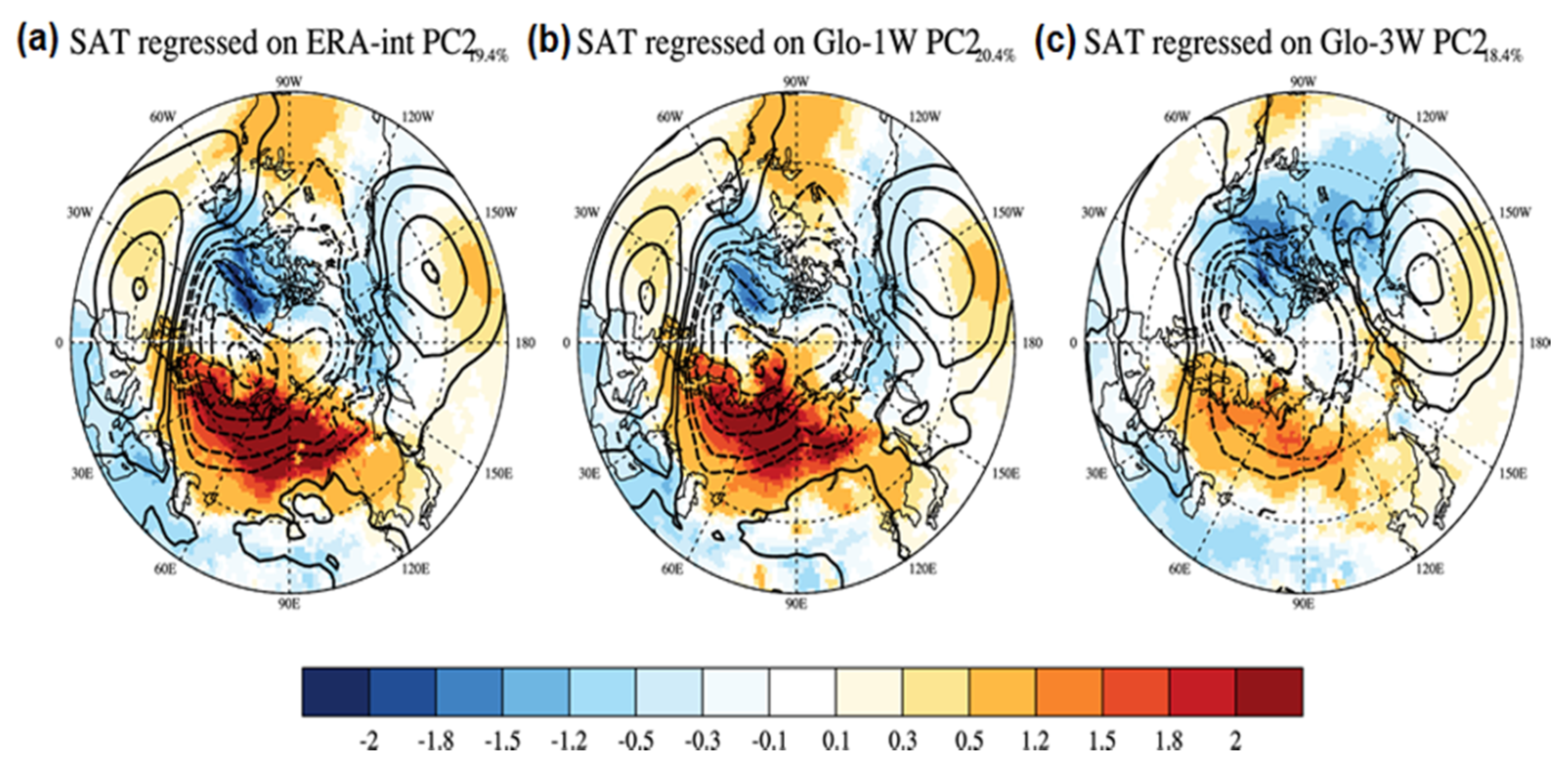
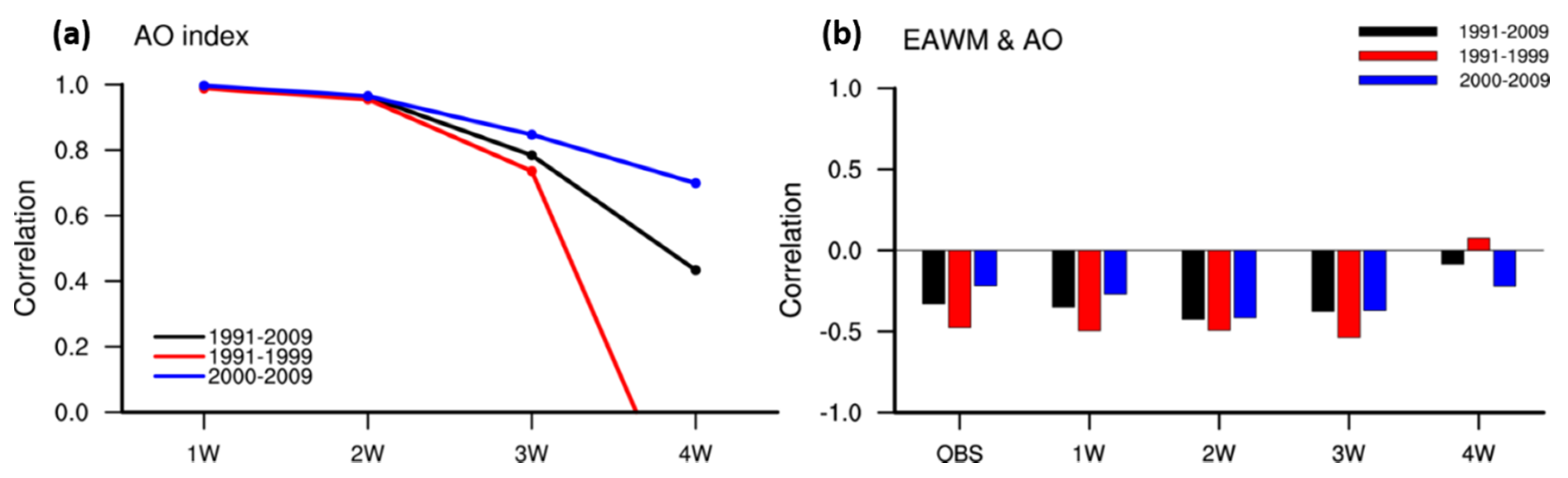
3.2. Effect of Arctic–Mid-Latitude Interaction on EAWM

Recently, many studies have discussed the effect of climate variability in the Arctic on the mid-latitudes [26,27,28,29]. These studies indicate that the temperature trends for the mid-latitudes and the Arctic show opposite patterns before and after the late 1990s. In the earlier period, the Arctic shows slight cooling, whereas in the later period, it shows rapid warming. It is well known that the recent cold winters in northern continents are related to Arctic warming; the so-called “warm Arctic–cold continent” pattern enforced via stationary Rossby waves. Labe et al. [29] recently mentioned that these Arctic–mid-latitude linkages show little connection with modeling results, although some model experiments support the observational evidence. To examine whether GloSea5 represents this recent phenomenon well, the linear trends for the surface temperature for the period 2000–2009, from ERA–Interim and GloSea5 with lead times of 1 and 3 weeks, are shown in Figure 6. The Arctic warming and Eurasian cooling trends shown in the reanalysis data are well simulated in the NWP for this period for a lead time of 1 week. The trend is well represented in the subseasonal period with a 3–week lead time, although the cooling strength is slightly weak.
To characterize the variability of the surface temperature over East Asia for the winter climate, an EOF analysis using surface temperature north of 20° N was applied. Figure 7 and Figure 8 show the sea level pressure and surface temperature regressed onto the first and second EOF analyses of surface temperature over the Arctic to the mid-latitudes, from the ERA-Interim and GloSea5 hindcasts, respectively. The first-mode eigenvector from ERA-Interim explains approximately 30% of the total variance. The first dominant structure of the EAWM is characterized by the strengthening of the Siberian high (Figure 7). This shows the cold temperatures in Eurasia to the East Asia continent, including the Korean peninsula, whereas there are the warm temperatures in the high-latitude regions. GloSea5 with a 1-week lead represents the pressure and temperature features from the observations well. The strengthening of the Siberian high and the cold temperature patterns are not captured by the increasing the lead time in GloSea5, although the warm temperature pattern is well represented. Consistently with other studies [29], Arctic-mid-latitude linkages tend to be weakened in the model experiment compared to the observational phenomena, especially with increasing lead times.
The second dominant structure of the EAWM, which explains approximately 20% of the total variance, shows an intensive pressure gradient forming between the Siberian high and the Aleutian low, associated with the main pattern of the EAWM (Figure 8). Gong et al. [30] found a significant out-of-phase relationship between the AO and the EAWM during the period 1951–1999. The negative phase of the AO is concurrent with a strong EAWM, though it could significantly influence the EAWM strengthening related to the Siberian high. Observation showed weakened sea level pressure and warm temperatures over the East Asia region. These patterns are exactly simulated by GloSea5 with a 1-week lead time. GloSea5 with a 3-week lead time generally captures the out-of-phase AO-EAWM relationship well, although its strength is weak.
Figure 9 shows the principal component (PC) time series of the first leading mode governing the detrended winter sea level pressure, from ERA-Interim and GloSea5 with lead times of 1 and 3 weeks. The PC time series from GloSea5 with a lead time of 1 week captures the interannual variation shown in the reanalysis data. However, the results from GloSea5 with a lead time of 3 weeks show a very different pattern from the observations, especially in the 2000s. The quantitative value of the Siberian high index is defined as the regional mean SLP averaged over the area 40–65° N and 80–120° E in winter, providing a measure of the strength of the Siberian high [31]. The interannual variation of the Siberian high index, representing the expansion or contraction of the Siberian high pressure, which is the characteristic most closely related to the first EOF mode from the surface temperature, is shown with a black dotted line in Figure 9. The time series of the Siberian high index is almost consistent with the observed pattern. In other words, it can be seen that the recent decrease in the EAWM prediction skill is also related to the failure of the simulation of the expansion or reduction of the Siberian high in GloSea5 with a lead time of 3 weeks.
The AO is a dominant pattern for the variation of sea level pressure from the Arctic to the mid-latitude region and is described by sea level pressure anomalies of one sign in the Arctic and anomalies of the opposite sign in the mid-latitudes [19]. To confirm the performance for the AO, which is a characteristic related to the second EOF mode from the surface temperature, the prediction skill of the AO index and the correlation between the EAWM and the AO based on the number of lead weeks are shown in Figure 10. The prediction skill of the AO index in the 2000s for GloSea5 is higher than in the 1990s and is especially low for a lead time of 4 weeks in the 1990s. It is a well-known fact that, through influencing large-scale circulations such as the Siberian high, a positive phase of winter AO generally leads to a weaker EAWM and warmer than normal winters.
It can be observed that the periods 1991–1999 and 2000–2009 show a negative correlation between the EAWM and the AO. The correlation between the AO and the EAWM in the earlier period tends to slightly decrease in the later period. The relationship in the earlier period is well simulated up to a lead time of 3 weeks; however, the weakened relationship in the later period is more strongly simulated than that observed for lead times of 2 and 3 weeks. Interestingly, for the 4−week lead time, although the correlation in the earlier period shows the opposite result, the correlation in the later period appears similar to the observation. Thus, the effect of the AO simulation on the recent decrease in the EAWM prediction skill in the 2000s, is not significant.

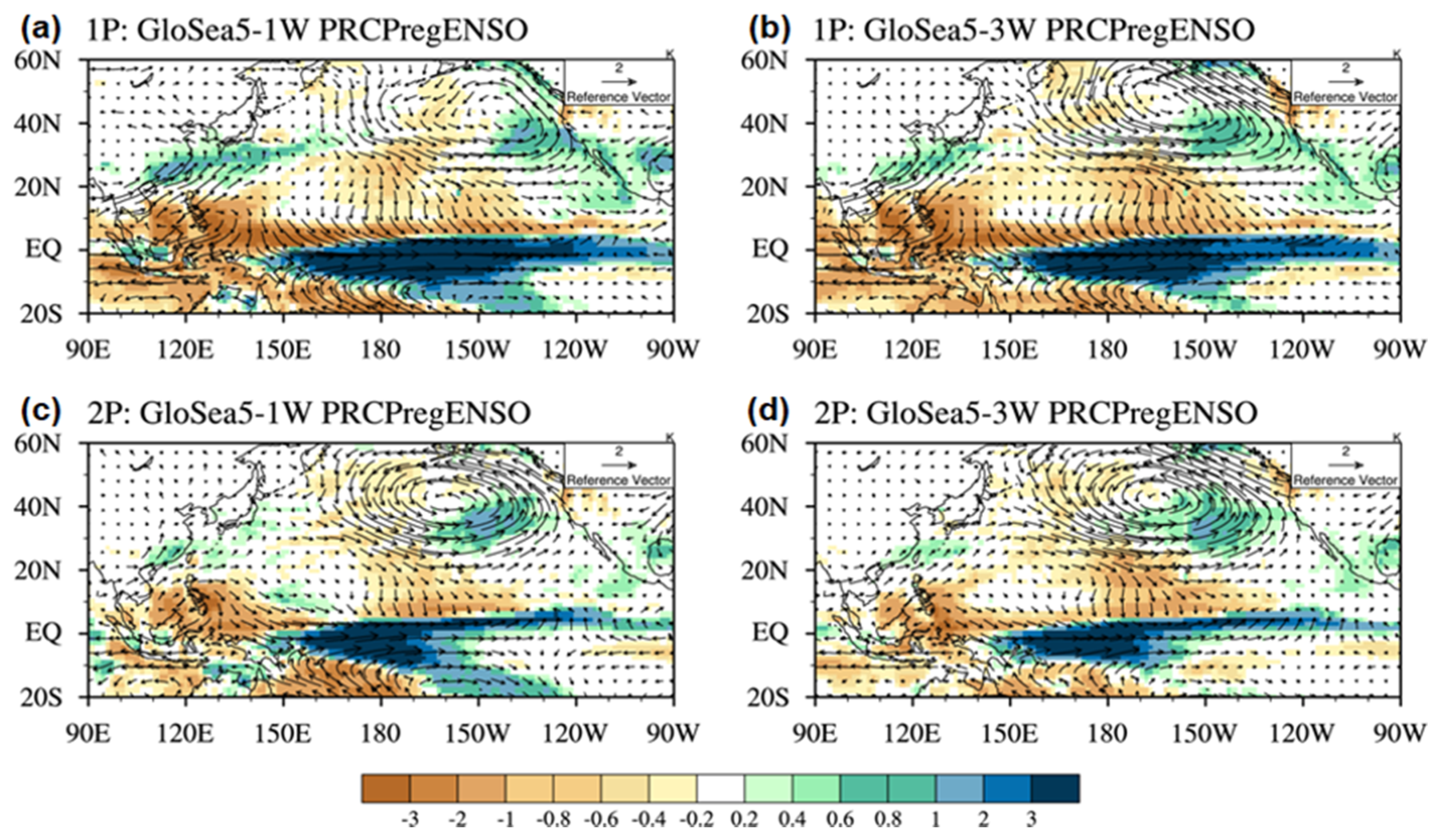
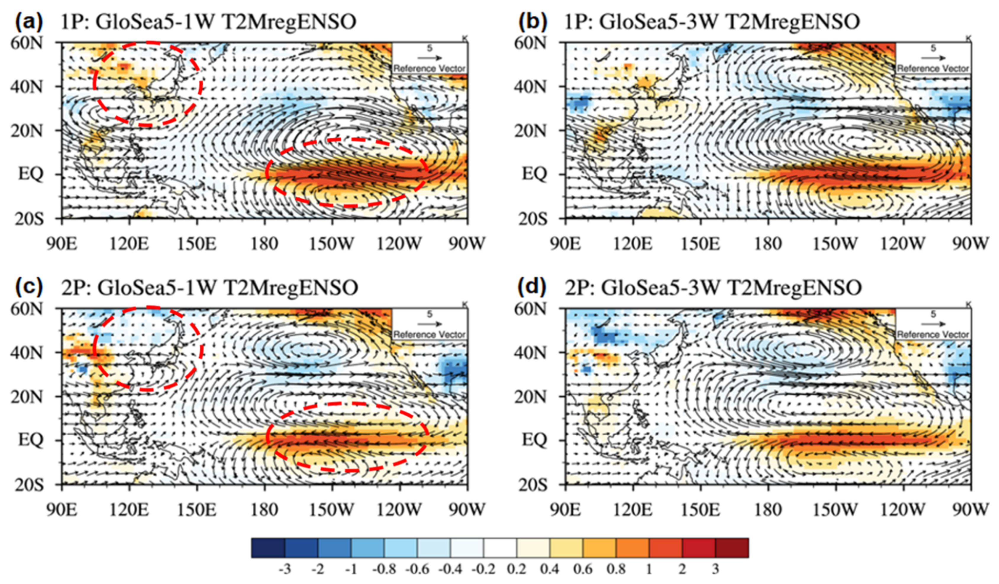
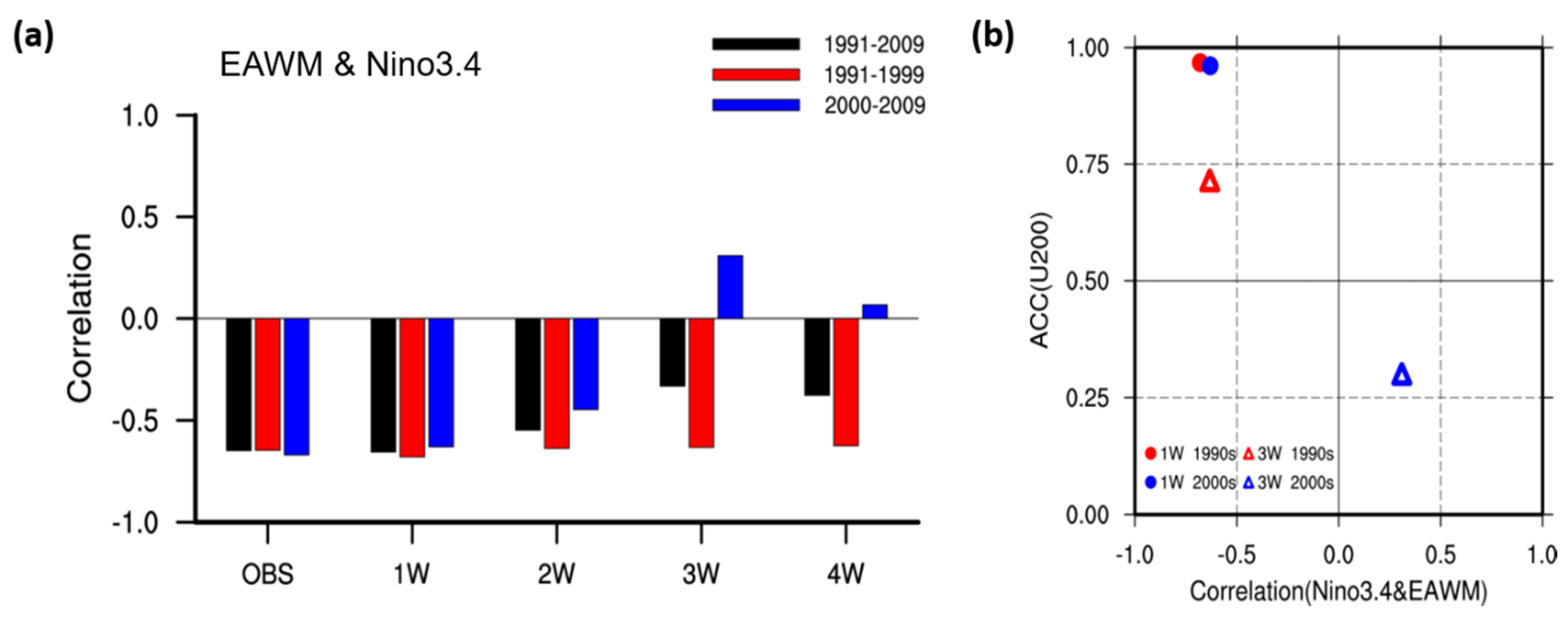
3.3. Effect of Tropics-Mid-Latitude Interaction on EAWM

It is well known that current seasonal prediction systems forecast the surface temperature reliably only in lower latitudes in the boreal winter. This is mainly driven by the extended prediction skill of ENSO, although the skill is very limited in the higher latitudes [32,33]. Therefore, the representation of the teleconnection from the tropics should be one of the key uncertainties in prediction systems. In addition, many studies have mentioned that the interannual variations of the EAWM are well correlated with ENSO [18,34,35]. The EAWM and ENSO show a negative correlation, associated with the anticyclonic circulation over the Philippine Sea, which is caused by warming in the central Pacific [35].
To examine the ENSO-related characteristics in the GloSea5 subseasonal prediction, the precipitation, temperature, and wind fields regressed to the Nino 3.4 index are shown in Figure 11 and Figure 12. The results from the ERA–Interim reanalysis are not shown, because the simulated pattern of association with the ENSO from GloSea5 with a lead time of 1 week mostly matched the observed pattern. In the early period, for positive cases of Nino 3.4 corresponding to the 850 hPa wind pattern related to the ENSO, precipitation decreases over the Maritime Continent and the western Indian Ocean and increases from southern China to southern Japan, compared to the negative cases. This is associated with weak westerlies over the subtropics and weak easterlies over the tropical Indian Ocean and the western North Pacific (Figure 11a). Even when the lead time increases, the relationship between the EAWM and the ENSO is generally well represented. However, the center of equatorial precipitation is weakened and wind circulation in the western North Pacific is overestimated (Figure 11b). In the later period, the center of the equatorial precipitation related to the ENSO shifts to the left, and the rainband from southern China to the south of Japan is weakened. In addition, the low-level circulation in the northeast Pacific is strengthened (Figure 11c). Changes in low-level circulation and precipitation patterns in the 2000s are well represented by GloSea5 with a lead time of 3 weeks (Figure 11d).
The surface temperature and upper-level circulation regressed onto the Nino 3.4 index are shown in Figure 12. In the earlier period, the high temperature over the central Pacific and the north–south dipole pattern of the upper-level circulation is related to the ENSO (Figure 12a). The temperature and the wind circulation from GloSea5 with a lead time of 3 weeks are generally well represented, although the wind circulation over the northwest Pacific is overestimated (Figure 12b). In the later period, the temperature peak over the central Pacific is shifted to the left and is weakened slightly, similarly to the precipitation pattern (Figure 12c). In addition, the circulation over the northeast Pacific is significantly strengthened and the East Asian jet is slightly weakened. It should be noted that GloSea5 with a lead time of 3 weeks underestimates the weakened circulation over East Asia and overestimates the strengthened circulation over the northeast Pacific (Figure 12d). Interestingly, the surface temperature over the central Pacific and the Korean Peninsula shows the same sign in the earlier period, whereas the sign is reversed in the later period.
The correlations between the EAWM and the Nino 3.4 index from observation and GloSea5, with various lead times, are plotted in Figure 13a. In the observation, both periods (1991–1999 and 2000–2009) show a negative correlation between the EAWM and Nino 3.4. In the earlier period, the correlation between the EAWM and the ENSO is generally well captured by GloSea5, even when the lead time is increased. However, the recent relationship between the EAWM and the ENSO simulated by GloSea5 is reduced rapidly as the lead time increases, showing different results from the observations. For GloSea5 with a 3-week lead time, the correlation is completely reversed. To examine the cause of the failure to represent this relationship, the prediction skill for the 200 hPa zonal wind over East Asia, which is highly related to the EAWM, is plotted in Figure 13b. As mentioned above, GloSea5 with a 3-week lead time shows a well-simulated 200 hPa zonal wind and relationship between the EAWM and Nino3.4 in the earlier period. However, the prediction skill for the 200 hPa zonal wind in GloSea5 with a 3-week lead time in the later period is significantly reduced as the lead time increases. In other word, it is clear that the failure to simulate the upper wind field in the later period is strongly related to the reduced prediction skill of the EAWM index.

4. Concluding Remarks

In this study, the characteristics of systematic errors in subseasonal predictions are investigated using an ensemble hindcast (1991–2010) produced by the KMA GloSea5. The KMA GloSea5 is a global prediction system for the subseasonal-to-seasonal time scale, based on a fully coupled atmosphere, land, ocean, and sea-ice model. To examine the fidelity of the prediction system in reproducing and forecasting phenomena, this study assesses the systematic biases in the global prediction model, focusing on the prediction skill for EAWM, which is a major driver of weather and climate variability in East Asia.
GloSea5 generally represents the observed temperature patterns well; however, there are clear cold biases over the continent in the northern hemisphere, including the East Asia region. In addition, the cold biases increase with increasing lead times. Although the pattern correlation coefficients of large-scale variables indicate great skill for lead times of 1 week, this reduces for lead times of 2 weeks onward. The EAWM index forecast from GloSea5, which is calculated from the upper-level zonal wind shear, represents the observed variation well with a 1-week lead in most years. GloSea5 with a 3-week lead shows a realistic representation of the variation; however, the recent EAWM prediction skill is quite poor.
To investigate the error characteristics of GloSea5, the hindcast period was analyzed by dividing it into two periods: 1991–2000 and 2001–2010. The results show that the prediction skill for the EAWM for a lead time of 3 weeks is significantly decreased in the 2000s compared to the 1990s, which is due to the weakening of the upper-level wind circulation over East Asia. In order to investigate the reason for the reduced EAWM prediction performance in the 2000s, the represented characteristics of the teleconnection relating to the polar and equatorial regions were examined. Although the prediction skill of GloSea5 for the AO index in the 2000s is higher than in the 1990s, the simulated excessive weakening of the East Asian jet related to the tropics and the failure to represent the Siberian high pressure related to the Arctic, are mainly responsible for the decreased EAWM prediction skill in the 2000s. In addition, one of the possible reasons for the low prediction skill of EAWM in the 2000s is that the observed characteristic, the peak of SST distribution in the equatorial Pacific moving from the east to the center, is weakly represented by GloSea5. This can affect the simulation of the large-scale circulation, which eventually leads to the mid-latitude variability.
This study evaluates the basic performance of the EAWM prediction using an ensemble hindcast produced by the KMA subseasonal prediction system. The study includes an identification and evaluation of systematic biases in the global prediction model, focusing on the prediction skill for the EAWM, with its interaction between the tropics and the Arctic climate. It is found that the main issue relating to the decreased prediction skill for the EAWM in the 2000s is the failure of the simulation of the East Asia upper-level circulation in the GloSea5 subseasonal prediction. Our study has a limitation in that there are recent studies for the S2S prediction skills of various modes of atmospheric variabilities (e.g., AO, ENSO, MJO, and QBO) [36,37,38]. In addition, the phase or amplitude of the AO and the ENSO can affect the various conditions with mid-latitude teleconnections. Nevertheless, our study suggests that the recent decrease in EAWM skill is significantly related to changes in the Arctic and the tropics, which is the most relevant mode of East Asia winter variability. However, the specific causes of the low prediction skill with regard to changes in equatorial surface temperature variability or Arctic-related circulation, need to be further investigated using a more comprehensive analysis. Consistently with this study, Hsu et al. [39] recently revealed that tropical sea surface temperature biases are related to the EAWM variability in the subseasonal simulation for 2011–2020. In this study, although the hindcast period is limited to 1991–2010 due to data availability, it will be extended to more recent periods (e.g., 2011–2020) after updating the model version.

Author Contributions

Conceptualization, S.H.; methodology, S.H.; software, S.H. and Y.J.; validation, S.H. and Y.J.; formal analysis, S.H.; investigation, S.H.; resources, S.H. and Y.J.; data curation, S.H. and Y.J.; writing—original draft preparation, S.H.; writing—review and editing, S.H.; visualization, S.H. and Y.J.; supervision, S.H.; project administration, S.H.; funding acquisition, S.H. and Y.J. All authors have read and agreed to the published version of the manuscript.

Funding

This research received no external funding.

Institutional Review Board Statement

The study was conducted according to the guidelines of the Declaration of Helsinki, and approved by the Institutional Review Board.

Informed Consent Statement

Informed consent was obtained from all subjects involved in the study.

Acknowledgments

This research was supported by the APEC Climate Center. This work is based on S2S data. S2S is a joint initiative of the World Weather Research Programme (WWRP). The original S2S database is hosted at ECMWF as an extension of the TIGGE database.

Conflicts of Interest

The authors declare no conflict of interest.

References

  1. Mariotti, A.; Ruti, P.M.; Rixen, M. Progress in subseasonal to seasonal prediction through a joint weather and climate community effort. npj Clim. Atmos. Sci. 2018, 1, 1–4. [Google Scholar] [CrossRef]
  2. Merryfield, W.J.; Baehr, J.; Batté, L.; Becker, E.J.; Butler, A.H.; Coelho, C.A.S.; Danabasoglu, G.; Dirmeyer, P.A.; Doblas-Reyes, F.J.; Domeisen, D.I.V.; et al. Current and emerging developments in subseasonal to decadal prediction. Bull. Amer. Meteor. Soc. 2020, 101, E869–E896. [Google Scholar] [CrossRef] [Green Version]
  3. Vitart, F.; Balsamo, G.; Buizza, R.; Ferranti, L.; Keeley, S.; Magnusson, L.; Molteni, F.; Weisheimer, A. Sub-Seasonal Predictions. ECMWF Tech. Memo., 738, 45. Available online: www.ecmwf.int/sites/default/files/elibrary/2014/12943-sub-seasonal-predictions.pdf (accessed on 5 October 2014).
  4. Mariotti, A.; Baggett, C.; Barnes, E.A.; Becker, E.; Butler, A.; Collins, D.C.; Dirmeyer, P.A.; Ferranti, L.; Johnson, N.C.; Jones, J.; et al. Windows of opportunity for skillful forecasts subseasonal to seasonal beyond. Bull. Amer. Meteor. Soc. 2020, 101, E608–E625. [Google Scholar] [CrossRef] [Green Version]
  5. Vitart, F.; Ardilouze, C.; Bonet, A.; Brookshaw, A.; Chen, M.; Codorean, C.; Déqué, M.; Ferranti, L.; Fucile, E.; Fuentes, M.; et al. The Subseasonal to Seasonal (S2S) Prediction Project Database. Bull. Amer. Meteor. Soc. 2017, 98, 163–173. [Google Scholar] [CrossRef]
  6. Saha, S.; Moorthi, S.; Wu, X.; Wang, J.; Nadiga, S.; Tripp, P.; Behringer, D.; Hou, Y.-T.; Chuang, H.-Y.; Iredell, M.; et al. The NCEP climate forecast system version 2. J. Clim. 2014, 27, 2185–2208. [Google Scholar] [CrossRef]
  7. MacLachlan, C.; Arribas, A.; Peterson, K.A.; Maidens, A.; Fereday, D.; Scaife, A.A.; Gordon, M.; Vellinga, M.; Williams, A.; Comer, R.E.; et al. Global Seasonal forecast system version 5 (GloSea5): A high-resolution seasonal forecast system. Quart. J. Roy. Meteor. Soc. 2015, 141, 1072–1084. [Google Scholar] [CrossRef]
  8. Williams, K.D.; Copsey, D.; Blockley, E.W.; Bodas-Salcedo, A.; Calvert, D.; Comer, R.; Davis, P.; Graham, T.; Hewitt, H.T.; Hill, R.; et al. The Met Office Global Coupled Model 3.0 and 3.1 (GC3.0 and GC3.1) Configurations. J. Adv. Modeling Earth Syst. 2018, 10, 357–380. [Google Scholar] [CrossRef]
  9. Waliser, D.E.; Li, J.-L.F.; L’Ecuyer, T.; Chen, W.-T. The impact of precipitating ice and snow on the radiation balance in global climate models. Geophys. Res. Lett. 2011, 38, L06802. [Google Scholar] [CrossRef]
  10. Koster, R.D.; Mahanama, S.P.P.; Yamada, T.J.; Balsamo, G.; Berg, A.; Boisserie, M.; Dirmeyer, P.; Doblas-Reyes, F.; Drewitt, G.; Gordon, C.T.; et al. Contribution of land surface initialization to subseasonal forecast skill: First results from a multi-model experiment. Geophys. Res. Lett. 2011, 37, L02402. [Google Scholar] [CrossRef] [Green Version]
  11. Sobolowski, S.; Glong, G.; Ting, M. Modeled climate state and dynamic responses to anomalous North American snow cover. J. Clim. 2010, 23, 785–799. [Google Scholar] [CrossRef]
  12. Woolnough, S.J.; Vitart, F.; Balmaseda, B.A. The role of the ocean in the Madden-Julian Oscillation: Implications for the MJO prediction. Quart. J. Meteor. Soc. 2007, 133, 117–128. [Google Scholar] [CrossRef]
  13. Wang, H.; Fan, K. Recent changes in the East Asian monsoon. Adv. Atmos. Sci. 2013, 37, 313–318. [Google Scholar]
  14. Miao, J.P.; Wang, T. Decadal variations of the East Asian winter monsoon in recent decades. Atmos. Sci. Lett. 2020, 21, e960. [Google Scholar] [CrossRef] [Green Version]
  15. Dai, G.; Li, C.; Han, Z.; Luo, D.; Yao, Y. The Nature and Predictability of the East Asian Extreme Cold Events of 2020/21. Adv. Atmos. Sci. 2021. [Google Scholar] [CrossRef]
  16. Zhou, W.; Li, C.; Wang, X. Possible connection between Pacific Oceanic interdecadal pathway and east Asian winter monsoon. Geophys. Res. Lett. 2007, 34, L01701. [Google Scholar] [CrossRef] [Green Version]
  17. Li, Y.; Yang, S. A dynamical index for the east Asian winter monsoon. J. Clim. 2010, 23, 4255–4262. [Google Scholar] [CrossRef]
  18. Jiang, X.; Yang, S.; Li, Y.; Kumar, A.; Wang, W.; Gao, Z. Dynamical prediction of the East Asian winter monsoon by the NCEP Climate Forecast System. J. Geophys. Res. Atmos. 2013, 118, 1312–1328. [Google Scholar] [CrossRef]
  19. Kim, H.M.; Webster, P.J.; Curry, J.A. Seasonal prediction skill of ECMWF System 4 and NCEP CFSv2 retrospective forecast for the Northern Hemisphere Winter. Clim. Dyn. 2012, 39, 2957–2973. [Google Scholar] [CrossRef] [Green Version]
  20. Ham, S.; Lim, A.-Y.; Kang, S.; Jeong, H.; Jeong, Y. A newly developed APCC SCoPS and its prediction of East Asia seasonal climate variability. Clim. Dyn. 2019, 52, 6391–6410. [Google Scholar] [CrossRef]
  21. Wang, L.; Chen, W. How well do existing indices measure the strength of the East Asian winter monsoon? Adv. Atmos. Sci. 2010, 27, 855–870. [Google Scholar] [CrossRef]
  22. Wang, L.; Chen, W.; Zhou, W. Effect of the climate shift around mid 1970s on the relationship between wintertime Ural blocking circulation and East Asian climate. Int. J. Clim. 2010, 30, 153–158. [Google Scholar] [CrossRef] [Green Version]
  23. Thompson, D.W.J.; Wallace, J.M. The Arctic Oscillation signature in the wintertime geopotential height and temperature fields. Geophys. Res. Lett. 1998, 25, 1297–1300. [Google Scholar] [CrossRef] [Green Version]
  24. Dee, D.P.; Uppala, S.M.; Simmons, A.J.; Berrisford, P.; Poli, P.; Kobayashi, S.; Andrae, U.; Balmaseda, M.A.; Balsamo, G.; Bauer, P.; et al. The ERA-Interim reanalysis: Configuration and performance of the data assimilation system. Quart. J. Roy. Meteor. Soc. 2011, 137, 553–597. [Google Scholar] [CrossRef]
  25. Adler, R.F. The Version 2 Global Precipitation Clilmatology Project (GPCP) monthly precipitation analysis (1979–Present). J. Hydrometeo. 2003, 4, 1147–1167. [Google Scholar] [CrossRef]
  26. Kug, J.-S.; Jeong, J.-H.; Jang, Y.-S.; Kim, B.-M.; Folland, C.K.; Min, S.-K.; Son, S.-W. Two distinct influences of Arctic warming on cold winters over North America and East Asia. Nat. Geosci. 2015, 8, 759–763. [Google Scholar] [CrossRef]
  27. Mori, M.; Watanabe, M.; Shiogama, H.; Inoue, J.; Kimoto, M. Arctic sea-ice influence on the frequent Eurasian cold winters in past decades. Nat. Geosci. 2014, 7, 869–873. [Google Scholar] [CrossRef]
  28. Cohen, J. Divergent consensuses on Arctic amplification influence on midlatitude severe winter weather. Nat. Clim. Chang. 2020, 10, 20–29. [Google Scholar] [CrossRef]
  29. Labe, Z.; Peings, Y.; Magnusdottir, G. Warm Arctic, cold Seberia pattern: Role of full Arctic amplification versus sea ice loss alone. Geophys. Res. Lett. 2020, 47, e2020GL088583. [Google Scholar] [CrossRef]
  30. Gong, D.; Wang, S.; Zhu, J. East Asian winter monsoon and Arctic Oscillation. Geophys. Res. Lett. 2001, 28, 2073–2076. [Google Scholar] [CrossRef]
  31. Hasanean, H.M.; Almazroui, M.; Jones, P.D.; Alamoudi, A.A. Siberian high variability and its teleconnections with tropical circulations and surface air temperature over Saudi Arabia. Clim. Dyn. 2013, 41, 2003–2018. [Google Scholar] [CrossRef]
  32. Wang, B.; Lee, J.-Y.; Kang, I.-S.; Shukla, J.; Park, C.-K.; Kumar, A.; Schemm, J.; Cocke, S.; Kug, J.-S.; Luo, J.-J.; et al. Advance and prospectus of seasonal prediction: Assessment of the APCC/CliPAS 14-model ensemble retrospective seasonal prediction (1980–2004). Clim. Dyn. 2009, 33, 93–117. [Google Scholar] [CrossRef] [Green Version]
  33. Lee, M.-I.; Kang, H.-S.; Kim, D.; Kim, D.; Kim, H.; Kang, D. Validation of the experimental hindcasts produced by the GloSea4 seasonal prediction system. Asia Pac. J. Atmos. Sci. 2014, 50, 307–326. [Google Scholar] [CrossRef]
  34. Kang, D.; Lee, M.-I. ENSO influence on the dynamical seasonal prediction of the East Asian Winter Monsoon. Clim. Dyn. 2017, 53, 7479–7495. [Google Scholar] [CrossRef]
  35. Wang, B.; Wu, R.; Fu, X. Pacific-East Asian teleconnection: How does ENSO affect East Asian climate? J. Clim. 2000, 13, 1517–1536. [Google Scholar] [CrossRef]
  36. Feng, P.N.; Lin, H.; Derome, J.; Merlis, T.M. Forecast skill of the NAO in the subseasonal-to-seasonal prediction models. J. Clim. 2021, 34, 4757–4769. [Google Scholar]
  37. Woolings, T.; Hannachi, A.; Hoskins, B. Variability of the North Atlantic eddy-driven jet stream. Quart. J. Meteor. Soc. 2010, 136, 856–868. [Google Scholar] [CrossRef] [Green Version]
  38. Yamagami, A.; Matsueda, M. Subseasonal Forecast Skill for Weekly Mean Atmospheric Variability Over the Northern Hemisphere in Winter and Its Relationship to Midlatitude Teleconnections. Geophys. Res. Lett. 2020, 47, e2020GL088508. [Google Scholar] [CrossRef]
  39. Hsu, L.-H.; Chen, D.-R.; Chiang, C.-C.; Chu, J.-L.; Yu, Y.-C.; Wu, C.-C. Simulations of the East Asian Winter Monsoon on Subseasonal to Seasonal Time Scales Using the Model for Prediction Across Scales. Atmosphere 2021, 12, 865. [Google Scholar] [CrossRef]
Figure 1. Spatial distribution of surface temperature biases (model minus ERA–Interim reanalysis) of (ad) lead times of 1–4 weeks for 1991–2009 DJF.
Atmosphere 12 01311 g001
Figure 2. Averaged pattern correlation coefficient (PCC) for (a) surface temperature, (b) 500 hPa geopotential height, (c) 850 hPa zonal wind, and (d) 200 hPa zonal wind. Pink, blue, green, and red dots indicate lead times of 1, 2, 3, and 4 weeks, respectively. Grey bars also indicate a lead time of 4 weeks.
Atmosphere 12 01311 g002
Figure 3. Time series of East Asia winter monsoon index as given by Li and Yang (2010) from ERA−Interim and GloSea5 with lead times of 1 (red) and 3 (blue) weeks.
Atmosphere 12 01311 g003
Figure 4. East Asia winter monsoon (EAWM) prediction skills from ERA–Interim and Glosea5 with lead times of 1–4 weeks. (Black), (red) and (blue) lines are averaged for 1991–1999, 1991–1999, and 2000–2009, respectively.
Atmosphere 12 01311 g004
Figure 5. Surface temperature (shaded) and 200 hPa zonal wind (contours) regressed on the East Asia winter monsoon (EAWM) from (a) ERA–Interim, (b) GloSea5 with a lead time of 1 week, and (c) GloSea5 with a lead time of 3 weeks.
Atmosphere 12 01311 g005
Figure 6. The linear trends in surface temperature during DJF for the period 2000–2009 from (a) ERA–Interim and GloSea5 with lead times of (b) 1 and (c) 3 weeks.
Atmosphere 12 01311 g006
Figure 7. Surface temperature (shaded) and sea level pressure (contours) regressed onto the EOF 1st PC from (a) ERA−Interim, (b) GloSea5 with a lead time of l week, and (c) GloSea5 with a lead time of 3 weeks.
Atmosphere 12 01311 g007
Figure 8. Surface temperature (shaded) and sea level pressure (contours) regressed onto the EOF 2nd PC from (a) ERA–Interim, (b) GloSea5 with a lead time of 1 week, and (c) GloSea5 with a lead time of 2 weeks.
Atmosphere 12 01311 g008
Figure 9. Leading mode governing detrended winter sea level pressure from ERA–Interim (black solid line), and GloSea5 with lead times of 1 week (blue line) and 3 weeks (red line). The black dashed line indicates the Siberian high index.
Atmosphere 12 01311 g009
Figure 10. (a) Correlation coefficient of the Arctic oscillation (AO) between ERA–Interim and GloSea5 with lead times of 1–4 weeks. (b) Relationship of AO and the East Asia winter monsoon (EAWM) index from ERA–Interim and GloSea5 with lead times of 1–4 weeks. Red bars are averaged for 1991–1999 and blue bars are averaged for 2000–2009.
Atmosphere 12 01311 g010
Figure 11. Surface precipitation (shaded) and 850 hPa wind (vectors) regressed onto the Nino 3.4 index from GloSea5 (a,c) with a lead time of 1 week, and (b,d) with a lead time of 3 weeks. In (a,b) 1P is averaged for 1991–1999, and in (c,d) 2P is averaged for 2001–2009.
Atmosphere 12 01311 g011
Figure 12. Surface temperature (shaded) and 200 hPa wind (vectors) regressed onto the Nino 3.4 index from GloSea5 (a,c) with a lead time of 1 week, and (b,d) with a lead time of 3 weeks. In (a,b) 1P is averaged for 1991–1999, and in (c,d) 2P is averaged for 2001–2009.
Atmosphere 12 01311 g012
Figure 13. (a) Correlation coefficient between Nino 3.4 index and East Asia monsoon index from ERA–Interim and GloSea5 with lead times of 1–4 weeks. (b) Anomaly correlation coefficient of 200 hPa zonal wind over East Asia with Nino 3.4 and EAWM indices. Red bars are averaged for 1991–1999, blue bars are averaged for 2000–2009.
Atmosphere 12 01311 g013
Publisher’s Note: MDPI stays neutral with regard to jurisdictional claims in published maps and institutional affiliations.

