Analysis of Spatio-Temporal Heterogeneity and Socioeconomic driving Factors of PM_2.5 in Beijing–Tianjin–Hebei and Its Surrounding Areas

Abstract

Due to rapid urbanization and socio-economic development, fine particulate matter (PM_2.5) pollution has drawn very wide concern, especially in the Beijing–Tianjin–Hebei region, as well as in its surrounding areas. Different socio-economic developments shape the unique characteristics of each city, which may contribute to the spatial heterogeneity of pollution levels. Based on ground fine particulate matter (PM_2.5) monitoring data and socioeconomic panel data from 2015 to 2019, the Beijing–Tianjin–Hebei region, and its surrounding provinces, were selected as a case study area to explore the spatio-temporal heterogeneity of PM_2.5 pollution, and the driving effect of socioeconomic factors on local air pollution. The spatio-temporal heterogeneity analysis showed that PM_2.5 concentration in the study area expressed a downward trend from 2015 to 2019. Specifically, the concentration in Beijing–Tianjin–Hebei and Henan Province had decreased, but in Shanxi Province and Shandong Province, the concentration showed an inverted U-shaped and U-shaped variation trend, respectively. From the perspective of spatial distribution, PM_2.5 concentrations in the study area had an obvious spatial positive correlation, with agglomeration characteristics of “high–high” and “low–low”. The high-value area was mainly distributed in the junction area of Henan, Shandong, and Hebei Provinces, which had been gradually moving to the southwest. The low values were mainly concentrated in the northern parts of Shanxi and Hebei Provinces, and the eastern part of Shandong Province. The results of the spatial lag model showed that Total Population (POP), Proportion of Urban Population (UP), Output of Second Industry (SI), and Roads Density (RD) had positive driving effects on PM_2.5 concentration, which were opposite of the Gross Domestic Product (GDP). In addition, the spatial spillover effect of the PM_2.5 concentrations in surrounding areas has a positive driving effect on local pollution levels. Although the PM_2.5 levels in the study area have been decreasing, air pollution is still a serious problem. In the future, studies on the spatial and temporal heterogeneity of PM_2.5 caused by unbalanced social development will help to better understand the interaction between urban development and environmental stress. These findings can contribute to the development of effective policies to mitigate and reduce PM_2.5 pollutions from a socio-economic perspective.

1. Introduction

With the advancement of industrialization and urbanization, many cities around the world are experiencing severe air pollution, especially particulate matter pollution. On a global scale, China, India, and South Asia have the most severe particulate matter pollution in the world [1]. In China, since 2011, Beijing–Tianjin–Hebei [2], the Yangtze River Delta [3], and other regions have experienced frequent smog, and air pollution has caused widespread concern. High concentrations of PM_2.5 can, not only accelerate the formation of haze but also significantly affect people’s health [4]. It has been proved that long-term exposure to high PM levels can easily cause a variety of diseases [5] and increase the risk of death [6]. In 2017, the State Ministry of Environmental Protection issued the “Beijing–Tianjin–Hebei and Surrounding Area Air Pollution Prevention and Control Work Plan in 2017”, which first proposed the concept of “2 + 26 cities” and implemented a large number of pollution control measures in these cities to alleviate air pollution in North China. Therefore, strengthening scientific understanding of the regulations of regional air particulate pollution will help to formulate urbanization policies and ensure that targeted air pollution control measures are properly implemented.

At present, research on PM_2.5 pollutions mainly focuses on temporal and spatial distribution rules [7], influencing factor analyses [8], source analyses [9], and health risk assessments [10] along with other aspects. Among them, influencing factors mainly include meteorological factors and socio-economic factors. Meteorological factors affect PM_2.5 concentration by changing its diffusion and chemical reaction conditions. Chen et al. [11] summarized the methods to quantify the impact of meteorological factors on PM_2.5 and comprehensively reviewed their impact mechanisms. Xu et al. [12] conducted a study on the temporal and spatial distributions of the influence of meteorological conditions on PM_2.5 concentration in China from 2000 to 2017, which showed an overall downward trend in PM_2.5 concentration, and the influence of meteorology varied greatly between different provinces. The socio-economic factors that directly or indirectly affect PM_2.5 concentration in the process of urbanization and economic development, include the national economy, industrial structure, population density, transportation, and other factors [13]. These factors mainly represent the impact of human activities on PM_2.5. The average urban PM_2.5 level is mainly affected by anthropogenic emissions of local air pollutants and the surrounding ecological level. Cheng et al. [14] used a dynamic spatial panel model to analyze the impact of foreign direct investment (FDI) on China’s PM_2.5 pollutions, and the results showed that FDI significantly aggravated China’s urban PM_2.5 pollutions. The study of Yan et al. [15] expressed that there was a heterogeneous relationship between PM_2.5 concentration and economic growth, urbanization, industrialization, and FDI and that population density had the greatest positive impact on PM_2.5 pollution. Zhang et al. [16] noted that PM_2.5 pollution was positively correlated with urbanization and road density, and negatively correlated with the proportion of tertiary industries.

Although many studies have been conducted on the temporal and spatial distributions of PM_2.5 and its influencing factors, the study areas of most studies mainly concentrate on the level of countries, urban agglomerations, and cities, while comparisons between regions are relatively rare. In addition, with rapid economic development, the North China region has been experiencing severe PM_2.5 pollution. Shanxi Province is located in the central region and has a decreasing economic development. Therefore, this study selects Beijing City, Tianjin City, Hebei Province, Henan Province, and Shanxi Province as the study areas. There are significant distinctions of PM_2.5 and economic development levels between the different cities, which provides advantages for studying the impact of socio-economic factors and spatial spillover effects on the PM_2.5 level. The aims of this study are: (1) explore the temporal and spatial distribution characteristics of PM_2.5 levels; (2) compare the spatial heterogeneity of PM_2.5 distribution characteristics in different regions, and (3) determine the influence of socio-economic factors and spatial spillover effects on PM_2.5 levels.

2. Materials and Methods

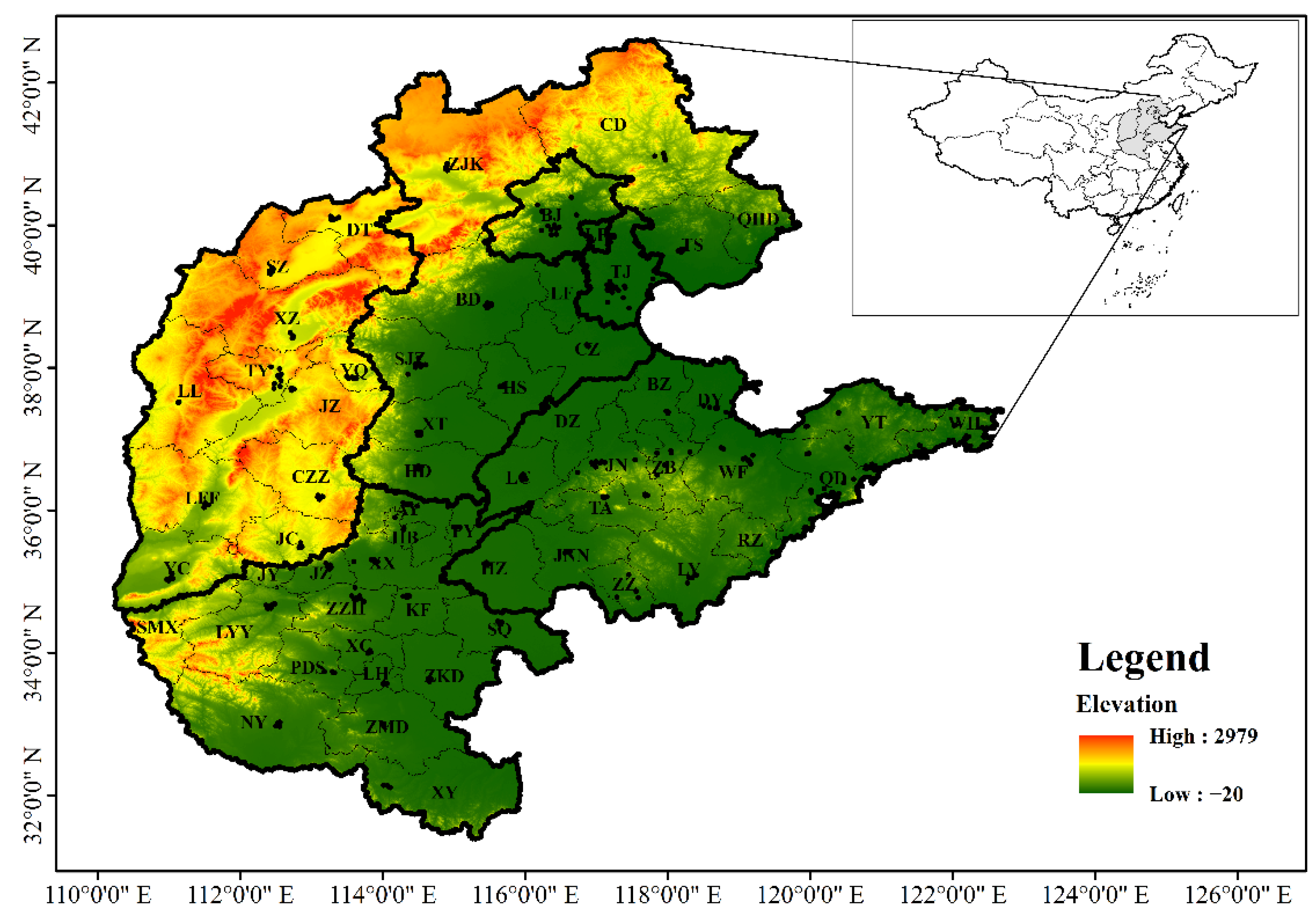
2.1. Study Area

This study selects Beijing City, Tianjin City, Hebei Province, Henan Province, and Shanxi Province as the study areas, which contains 56 cities in four provinces and two municipalities, as shown in Figure 1. Among them, Hebei Province, Shandong Province, Shanxi Province, and Henan Province have 11, 16, 11, and 18 prefecture-level cities, respectively. The names and abbreviations of all cities are shown in Table S1. The study area is located between 31°23′ N–42°40′ N and 110°14′ E–122°42.3′ E in China, with the Loess Plateau in the west and the North China Plain in the east. With its rapid economic development and rapid consumption of energy, the air quality in North China is not better and haze pollution incidents occur frequently; this area is considered one of the most polluted areas of China. In addition, the study area includes, not only the eastern regions with their rapid economic development, such as the Beijing–Tianjin–Hebei urban agglomeration and Shandong Province but also the central regions with slower economic development speeds, such as Shanxi Province. The socio-economic development of the study area is very unbalanced, which provides favorable conditions for analyzing the influence of socio-economic factors on PM_2.5 concentration. Therefore, this paper selects four provinces and two municipalities as the study areas to explore the temporal and spatial heterogeneity of PM_2.5 and the influence of socioeconomic factors on PM_2.5 concentrations in 2015–2019.

2.2. Data Sources and Validity

This study collected hourly PM_2.5 concentration data from 347 automatic air quality monitoring stations in the study area, from 1 January 2015, to 31 December 2019. This set of data was obtained from the Urban Air Quality Distribution platform of the National Environmental Monitoring Center (http://www.moc.cma.gov.cn, accessed on 9 October 2021). Based on the hourly PM_2.5 data, the arithmetic mean method was used to calculate the annual PM_2.5 concentration in each city, from 2015 to 2019. To improve the validity of the data, we processed the missing values according to the provisions of the Ambient Air Quality Standard (GB3095−2012). When calculating the daily average concentrations, we required that the number of hourly average concentrations or the sampling time should be more than 20, otherwise the daily average concentration was considered invalid. In calculating the average monthly concentrations, we required at least 27 (February: 25) daily average concentration values, otherwise, the monthly mean concentration was considered invalid. At least 324 daily average concentrations were required to calculate the annual average concentration, otherwise, the annual average concentration was considered invalid.

The potential impact of socioeconomic indicators on PM_2.5 pollution has been widely discussed. Based on previous studies and the availability of socioeconomic data, we selected seven indicators (

Table 1. Socioeconomic indicators and the abbreviations and units.

Category	Variable	Abbreviation	Units
Independent variable	PM2.5 concentration	PM2.5	μg/m3
Dependent variable	Total Population	POP	104 persons
	Gross Domestic Product	GDP	104 CNY
	Green Ratio of Built-up Area	GR	%
	Output of Second Industry	SI	104 CNY
	Proportion of Urban Population	UP	%
	Roads Density	RD	km/km2
	Proportion of Built-up Area	BA	%

): Population (POP), Gross Domestic Product (GDP), Green Ratio of Built-up Area (GR), Output of Second Industry (SI), Proportion of Urban Population (UP), Roads Density (RD), and Proportion of Built-up Area (BA). Among them, POP, GDP, and GR, respectively, represent population size, economic development level, and urban greening; SI and RD express industrial structure and traffic factors, respectively; UP and BA represent population urbanization and spatial urbanization. The annual statistical data of POP, GDP, SI, and RD were acquired from the Social and Economic Development Bulletin and Statistical Yearbook of each city in the study area, while those of GR and BA were obtained from the China Urban Statistical Yearbook. The time span of all socioeconomic indicators was consistent with that of PM_2.5 data in this study. Figure S4 provides detailed statistical information on these socioeconomic factors, for each city.

2.3. Statistical Methods

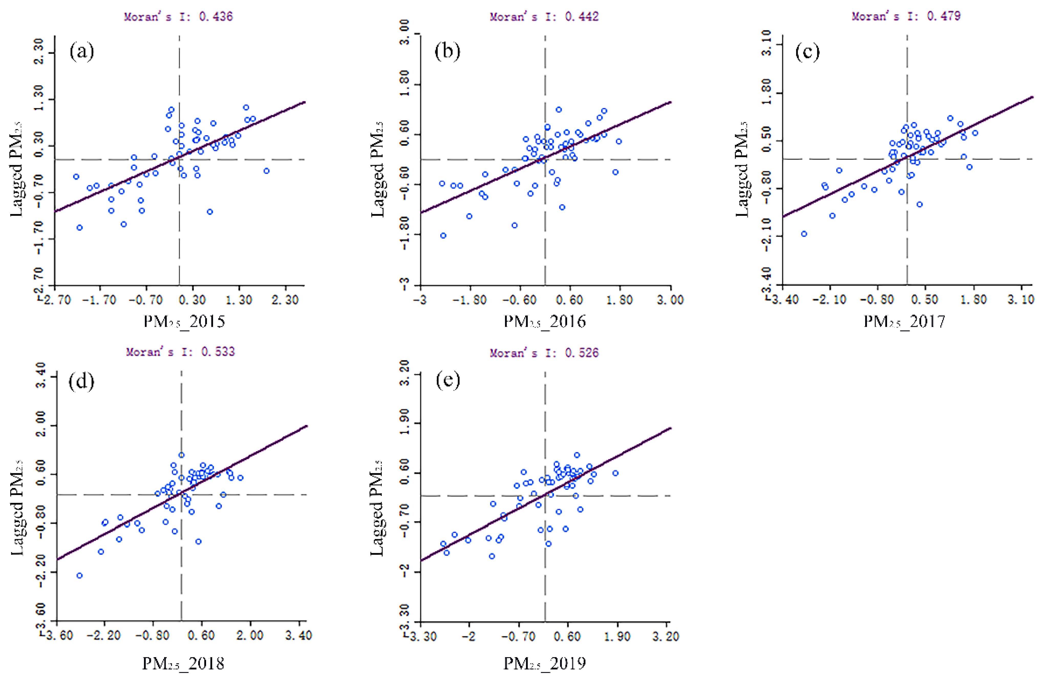
2.3.1. Moran’s I Test

Air pollution usually has obvious spatial distribution characteristics with regional aggregation. Many researchers usually use Moran’s I to test the spatial correlation of variables. In this study, we used the Global Moran’s I to test the overall spatial effect of PM_2.5 concentrations in 58 cities, from 2015 to 2019. The Global Moran’s I model can be explained as follows [17]:

$$GlobalMora{n}^{\prime }\mathrm{s}{I}_i=\frac{n{\sum }_{i=1}^n{\sum }_{j=1}^n{w}_{ij}\left(y_i-\overline{y}\right)\left(y_j-\overline{y}\right)}{S_0{\sum }_{i=1}^n{\left(y_i-\overline{y}\right)}^2}$$

(1)

$$Z=\frac{1-E\left(I\right)}{\sqrt{Var\left(I\right)}}$$

(2)

$$E\left[I\right]=-1/\left(n-1\right)$$

(3)

$$V\left[I\right]=E\left[I^2\right]-E{\left[I\right]}^2$$

(4)

where y_i is the PM_2.5 concentration of city i, y_j is the PM_2.5 concentration of city j, and $\overline{y}$ is the average PM_2.5 concentration of the study area. w_ij is the spatial weight matrix; if two cities share a common boundary, the weight is 1, otherwise, it is 0; $S_0={\sum }_{i=1}^n{\sum }_{j=1}^n{w}_{ij}$ is the aggregation of all spatial weights; n = 56 is the number of cities. Z score and p values used to judge the Moran’s I significance level; when the |Z| > 1.96 or p < 0.05, the result is considered significant at the 95% confidence level; when the |Z| > 2.58 or p < 0.01, the result is considered significant at the 99% confidence level. In this paper, the Global Moran’s I was calculated using ArcGIS software.

2.3.2. Hot Spot Analysis

Hot Spot Analysis is often used to identify potential spatial agglomeration characteristics of PM_2.5 pollution, and PM_2.5 levels are divided into cold spots, insignificant points, and hot spots. The Getis-Ord Gi* of ArcGIS was used to calculate the Gi* of each city in the study area. The principle formulae are as follows [18]:

$$G_i^{*}=\frac{{\sum }_{j=1}^n{w}_{ij}{x}_j-\overline{x}{\sum }_{j=1}^n{w}_{ij}}{S\sqrt{\frac{\left[n{\sum }_{j=1}^n{w}_{ij}^2-{\left({\sum }_{j=1}^n{w}_{ij}\right)}^2\right]}{n-1}}}$$

(5)

$$S=\sqrt{\frac{{\sum }_{j=1}^n{x}_j^2}{n}-{\left(\overline{x}\right)}^2}$$

(6)

where x_j is the annual PM_2.5 concentration of city j; ω_ij is the spatial weight between city i and city j, and n = 56 represents the number of cities in the study area.

2.3.3. Spatial Lag Model

Socioeconomic variables, such as GDP, population size, and traffic, greatly affect local PM_2.5 concentrations. In this study, the Spatial Lag Model (SLM) was used to determine the influence of different socio-economic factors on PM_2.5 concentration, which could be explained by Formula (7):

$$Y=\rho WY+X\beta +\epsilon , \epsilon ~N\left[0,{\sigma }^{2}I\right]$$

(7)

where Y indicates the PM_2.5 concentration; X expresses the independent variables, including all introduced socioeconomic factors; ρ is the spatial effect coefficient, and its value ranges from 0 to 1. The spatial matrix is represented by W, which indicates whether two spatial elements have a common boundary; β represents the regression coefficient of explanatory variables; and ε is the error term.

3. Results and Discussion

3.1. Temporal Variation Characteristics of PM_2.5

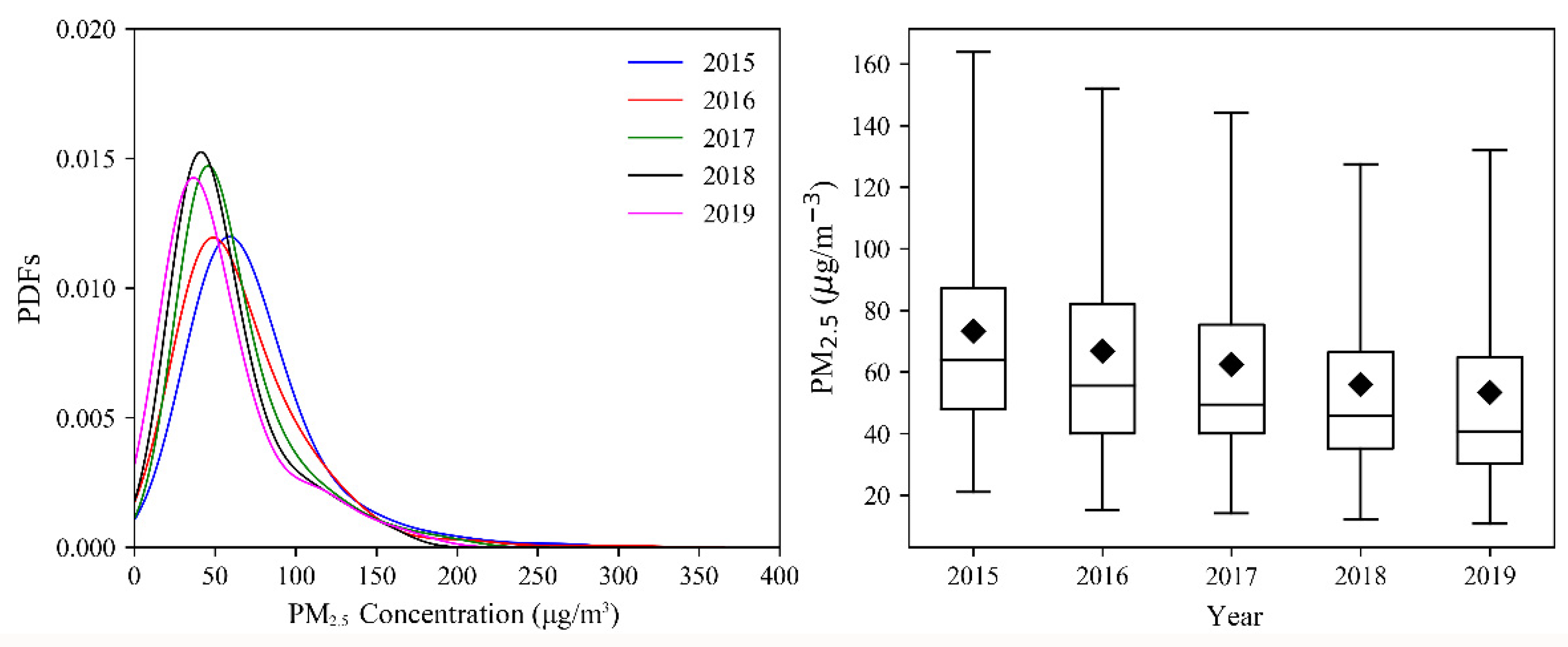
3.1.1. Temporal Variation Trend of PM_2.5 Concentration

The variation trend of PM_2.5 concentration in the study area was determined by calculating the Probability Density Functions (PDFs) and annual average concentrations of PM_2.5 in the study area, from 2015 to 2019. As shown in Figure 2, the PM_2.5 concentration in the study area expressed a downward trend from 2015 to 2019, which decreased by 27.17%, from 73.23 μg/m³ in 2015 to 53.34 μg/m³ in 2019. Although the annual PM_2.5 concentration decreased, it still exceeded the Grade II standard of PM_2.5 (35 μg/m³) in the Ambient Air Quality Standard (GB3095-2012) in 2019, which indicated that PM_2.5 pollution in the study area was still severe. The frequency distribution of PM_2.5 can be found in the PDF graph. From 2015 to 2019, the probability density curve moved to the left as a whole, indicating that PM_2.5 concentration had decreased in all concentration intervals. The curves of 2015 and 2016 are similar, while those of 2017, 2018, and 2019 are similar. Compared with 2016, the occurrence probability of high concentration decreased significantly in 2017, resulting in a significant increase in probability in the low concentration intervals, and then remained stable. This sudden change may be related to the stricter air pollution control measures that were implemented in 2017.

The mitigation trend was more significant in the context of concentration levels. In 2015, the average annual concentration of PM_2.5 in all cities ranged from 34.6 to 106.42 μg/m³, but was 26.52–72.39 μg/m³ in 2019. We can find that there was a large difference between different cities, with the maximum concentration being about three times that of the minimum. During the period of 2015–2019, the maximum concentration occurred in BD in 2015 and the minimum concentration occurred in WH in 2018. In addition, we also determined the statistics on the percentage of exceeding standard days in each city, from 2015 to 2019, as shown in Figure S1. In 2015, the average percentage of exceeding standard days in the study area was 37.45%, but it dropped to 15.66% in 2019. This apparent mitigation of PM_2.5 pollution did not just start in 2015, it had been going on for a long time. Some studies on the long-term variation trends of PM_2.5 concentrations have shown that it had been increasing since 2000 until reaching a peak in 2008, and then it fluctuated continuously and reached another peak in 2014 before decreasing since then [19]. It fluctuated after 2008 as the harm of PM_2.5 pollution was widely known after the Beijing Olympic Games and China gradually entered the stage of economic restructuring [20]. China’s government began to implement strict pollution control measures and regarded PM_2.5 as a routine monitoring pollutant after issuing the Action Plan for Air Pollution Prevention and Control in 2013, which may be why PM_2.5 concentration continued to decrease after 2014 [21]. As a large number of emission reduction measures have already been implemented, the reduction in PM_2.5 will gradually reduce in the future. Therefore, the speed of pollution mitigation may be slowed down, and the spatial difference between cities would become narrower. From this aspect, Jiang et al. [22] reported that there was a spatial convergence trend for PM_2.5 concentrations in the Beijing–Tianjin–Hebei region.

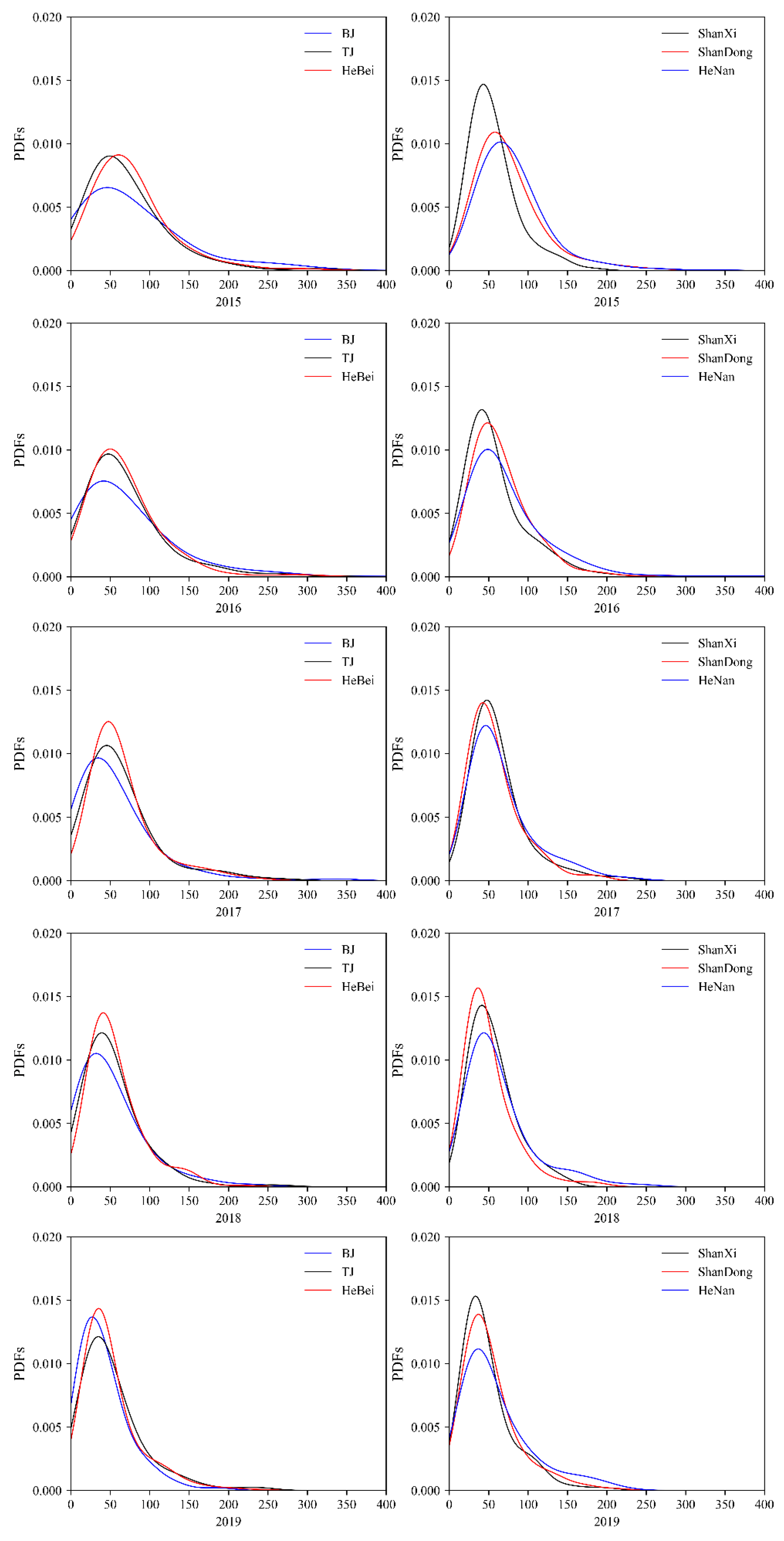
3.1.2. The Spatial Heterogeneity of Temporal Variations

Although PM_2.5 concentrations in the study area have been decreasing on the whole, they express different temporal regulations in various areas. As shown in Figure S2, Beijing, Tianjin, and most cities in Hebei and Henan Provinces decreased from 2015 to 2019, while a few cities showed different patterns. The average concentrations in Hebei Province and Henan Province also had the same patterns as most of the cities under their jurisdictions. However, the patterns of cities in Shanxi Province and Shandong Province were quite different from the others. To be more specific, PM_2.5 concentrations in Shanxi Province first went up but then decreased, and reached their highest level in 2017, presenting an inverted U-shaped trend. In Shandong Province, it first went down, and then it went up, reaching the lowest level in 2018 and showing a U-shaped trend. The patterns of most cities in the two provinces were consistent with their corresponding provinces. This heterogeneity may be related to differences in economic development, environmental protection policies, geographical differences, and other factors between the different provinces. The regions with the highest PM_2.5 concentration in 2015 were Beijing and Henan Provinces, and Henan Province exhibited the highest PM_2.5 concentration for the period of 2016–2019. After five years of decline, Beijing ranked last among the four provinces and two municipalities in 2019.

Specific to the urban level, the discrepancies in the reduction rates among different regions were more obvious, as shown in Figure S3. Specifically, BJ, BD, LF, DZ, and LC exhibited the highest reduction rate if more than 40%. Those of TY, YQ, JC, YC, and LFF were slightly less than 10%. The former was mainly concentrated in the Beijing–Tianjin–Hebei region, while the latter was under the jurisdiction of Shanxi Province. To further explore the differences in temporal variations, we plotted the PDFs of PM_2.5 in each province or municipality from 2015 to 2019, as shown in Figure 3. To facilitate comparison, we divided the study area into the Beijing–Tianjin–Hebei region and its surrounding regions (Shandong, Hebei, Shanxi Province). In 2015, the PDFs of each province varied greatly. Shanxi Province had the highest peak value, while Beijing had the lowest. Although the concentration ranges of the two peak areas were similar, the occurrence probability of high PM_2.5 concentration in Beijing was high, indicating that Beijing was prone to PM_2.5 pollution events. On the whole, the peaks in the Beijing–Tianjin–Hebei region were lower, while those in the surrounding region were higher, indicating that PM_2.5 pollution in the Beijing–Tianjin–Hebei region was more serious than in its surrounding areas. From the temporal point of view, the curve variation of the Beijing–Tianjin–Hebei region is very significant, especially in terms of BJ. The Shandong, Henan, and Shanxi regions also showed a trend of pollution alleviation. It is worth noting that the PDFs curve of Henan Province was always at the bottom, indicating that it had higher PM_2.5 pollution. After five years of improvement, the PDFs curves of the six regions showed a tendency to gradually coincide. Until 2019, the curves were quite similar, showing that the spatial differences of PM_2.5 concentration were narrowing, which is similar to the research results of Jiang, He, and Zhou [22].

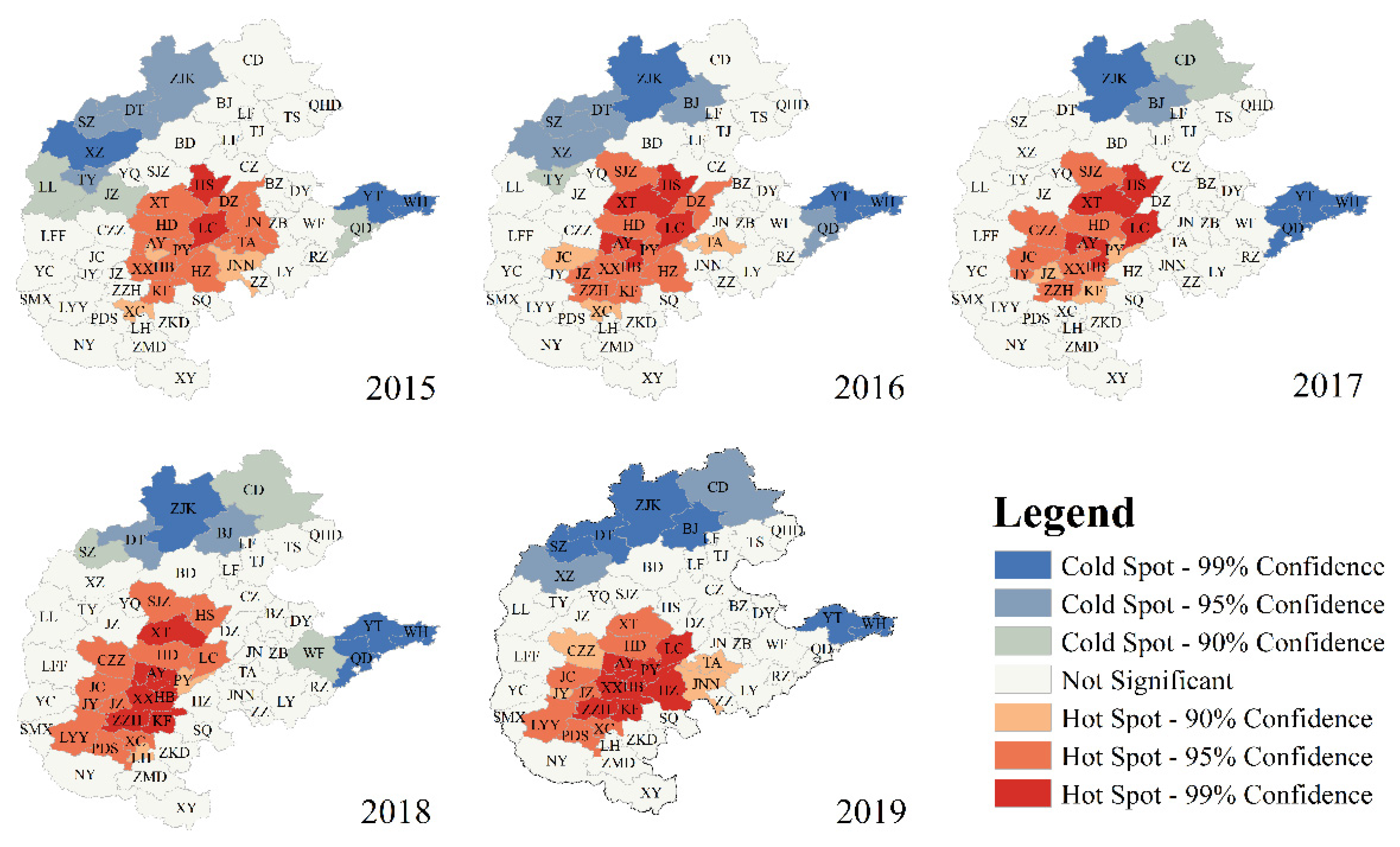
3.2. Spatial Variation Trend of PM_2.5

To determine the spatial distribution characteristics of PM_2.5 concentrations in the study areas, we calculated the Global Moran’s I during 2015–2019. As shown in

Table 2. Global Moran’s I from 2015 to 2019.

Year	I	p-Value	Z-Score
2015	0.372501	0.000001	4.855292
2016	0.344208	0.000006	4.532812
2017	0.363731	0.000002	4.796205
2018	0.389324	0.000000	5.123085
2019	0.414598	0.000000	5.429379

, with p-values < 0.01 and Z-score > 2.58, the Global Moran’s I was acceptable. From 2015 to 2019, the PM_2.5 concentrations in the study areas showed a significant positive spatial correlation, which indicated that the diffusion of PM_2.5 concentrations between cities was not random, and rather showed similar spatial connections and tended to aggregate. This spatial correlation has been gradually increasing since 2016. To better exhibit the agglomeration characteristics of the study area, we drew a Moran scatter diagram, as shown in Figure 4. Most cities are concentrated in the first and third quadrants, and only a few cities appear in the second and fourth quadrants which indicate that PM_2.5 pollution in the study areas presented obvious “high–high” and “low–low” agglomeration. This spatial characteristic is caused by the unbalanced economic development in the earlier period. With the sustainable development of the economy and the transformation of urban planning and layout, it would change.

To clearly determine the high and low concentration areas of PM_2.5 pollution, we drew a Getis-Ord Gi* statistical graph for the study area during 2015–2019, as shown in Figure 5. On the whole, the cold spots in the study area were mainly distributed in the north of Shanxi and Hebei Provinces, and the eastern coastal areas of Shandong Province and the hot spots were mainly concentrated in the junction area of Hebei, Shandong, and Henan Provinces. In terms of temporal change, the cold spots gradually shifted from the northwest to the north of the study area, while those in the eastern coastal region of Shandong Province were composed of YT, QD, and WH with no change. Additionally, the hot spot moved to the southwest gradually from 2015 to 2019. This moving of the PM_2.5 pollution center does not mean that the air quality in hot spots city were getting worse. In fact, almost all cities had been experiencing PM_2.5 pollution alleviation at different levels. The PM_2.5 concentration in some cities, such as SJZ, JN, and DZ, decreased sharply from hot spots to insignificant spots; some cities, such as JY, LYY, and PDS, declined slowly from insignificant spots to hot spots. This conversion of hot and cold spots is essentially determined by the transformation of the local industrial structure and the implementation of environmental protection policies. In fact, the upgrading and relocation of heavily polluting enterprises in the Beijing–Hebei–Tianjin region may also be one of the reasons for the moving of the pollution centroid. XT, HD, LC, AY, KF, PY, HB, XX, and other cities had always been hot spot cities during 2015–2019, indicating that the pollution in these cities was relatively serious and that control measures still needed to be taken for reducing the PM_2.5 pollution risk level.

3.3. Analysis of Socioeconomic Influence Factors

Different socioeconomic indicators reflect different human activities, which could affect the spatial and temporal heterogeneity of PM_2.5 concentrations to various degrees. In this study, we used a spatial lag model (SLM) to determine the impact of various socioeconomic factors on PM_2.5 concentrations. To ensure the data conformed to the normal distribution, a logarithmic transformation was performed on the socioeconomic data and PM_2.5 concentrations before using SLM.

Table 3. Results of spatial lag model.

	2015		2016		2017		2018		2019
Variable	Coefficient	Probability	Coefficient	Probability	Coefficient	Probability	Coefficient	Probability	Coefficient	Probability
ρ	0.560	0.000 **	0.583	0.000 **	0.739	0.000 **	0.724	0.000 **	0.574	0.000 **
GDP	−0.405	0.005 **	−0.328	0.088	−0.489	0.001 **	−0.364	0.012*	−0.415	0.002 **
POP	0.222	0.001 **	0.195	0.047 *	0.289	0.000 **	0.244	0.003 **	0.243	0.002 **
UP	0.085	0.010 *	0.225	0.317	0.422	0.039 *	0.351	0.091	0.339	0.080
SI	0.375	0.007 **	0.238	0.110	0.323	0.005 **	0.202	0.062	0.248	0.018 *
RD	0.337	0.000 **	0.271	0.000 **	0.163	0.011 *	0.146	0.020 *	0.218	0.001 **
BA	−0.036	0.199	−0.020	0.480	−0.029	0.193	−0.005	0.831	0.015	0.533
GR	0.217	0.332	−0.112	0.560	−0.132	0.631	−0.166	0.582	−0.163	0.595

**: Significant at 0.01 levels; *: significant at 0.05 levels.

shows the quantified results of the SLM model from 2015 to 2019.

The spatial lag model introduced the spatial effect coefficient ρ to characterize the influence of PM_2.5 levels from the surrounding areas on the local area. From 2015 to 2019, there was a positive relationship between PM_2.5 concentration in local and surrounding regions, indicating that local PM_2.5 levels were significantly influenced by surrounding areas. This is consistent with the “high–high” and “low–low” agglomeration characteristics of PM_2.5 concentrations in the study area. Local PM_2.5 pollution was not only related to local pollutant emissions but was also affected by pollution transport from other regions. Dong et al. [23] studied the pollution transmission contribution in the Beijing–Tianjin–Hebei region and the results showed 32.5% to 68.4% contribution of PM_2.5 transmission in 2017. Local emission sources remain important contributors to the Beijing–Tianjin–Hebei region but the interactions between cities are also strong.

GDP represents the local economic development level. Except for 2016, GDP showed a significant negative correlation with the PM_2.5 level, indicating that economic development had a certain inhibitory effect on PM_2.5 pollution in the study area. As an economy grows, local investment in air pollution control will also increase. In addition, a relatively developed economy is conducive to effective integration and utilization of resources, affecting the local industrial structure and urban layout. Dong et al. [24] found that economic development and industrial upgrading were the main driving forces for haze pollution improvement in China’s regions, while the transportation industry and construction industry were the two major sources of PM_2.5 pollution. This is consistent with our findings, but other studies have shown different results. Yan, Kong, Jiang, Huang, and Ye [13] observed that the impacts of economic development on PM_2.5 pollution varied with the degree of development. Economic development can alleviate PM_2.5 pollution in developed areas, while it can promote PM_2.5 pollution in underdeveloped areas. As noted by the theory of the Environmental Kuznets Curve (EKC), a later stage of urbanization is ultimately conducive to alleviating the pollution caused by the early stage of urbanization, and there is a threshold of an inflection point in the middle. Wang et al. [25] explained this in detail and obtained similar results to us.

Over 2015–2019, POP and PM_2.5 levels showed a positive correlation, passing the significance test, indicating that population growth contributed to the formation of urban PM_2.5 pollution. The increase in the population size resulted in growing demands for employment, housing, transportation, and energy consumption; thus, promoting the emission of pollutants. Han et al. [26] analyzed the relationship between population variations and PM_2.5 levels, and the results showed that there was a positive trend between population and PM_2.5 in most cities in China and that the contribution rate of megacities was 5.40 ± 4.80 μg/m³ per million people. However, there was also a negative trend between population size and PM_2.5 in some regions [13], because megacities with dense populations help to integrate resources and improve the utilization efficiency of urban infrastructure and natural resources, thus reducing PM_2.5 pollution.

UP refers to the proportion of the urban population in the total population, which is usually used to represent the level of urbanization. The results of Table 3 indicate that UP had a positive impact on PM_2.5 pollution in 2015 and 2017, but did not pass the significance test in other years. The growth or aggregation of an urban population usually leads to an increase in automobiles, housing and energy consumption, industrial production, and construction activities, which would have an impact on the increase in PM_2.5 concentrations. Relevant studies [27] showed that the relationship between the proportion of the urban population and ecological environment pressures in the Beijing–Tianjin–Hebei region also conformed to the EKC theory, and it could effectively alleviate ecological environment pressure until it reached 80%, which was the turning point in EKC for most cities. By 2019, the proportion of the urban population in BJ and TJ exceeded 80%, while others were within the scope of 40–60%, below the threshold, indicating that we still have a long way to go in the urbanization process.

SI is the value-added of Secondary Industry and is used to represent the industrial structure. There was a significant positive correlation between SI and PM_2.5 concentrations in 2015, 2017, and 2019. According to the statistical results of the output of the secondary industry, as shown in Figure S4, it had been decreasing or first increasing and then decreasing in AY, BJ, BD, LC, JNN, LF, PY, SJZ, TJ, and TA during 2015–2019, while it increased in other cities. These cities were often accompanied by severe PM_2.5 pollution, which indicated that these cities may have already carried out the elimination of backward production capacity or the transfer of secondary industry to alleviate local PM_2.5 pollution. The national development strategy has significantly increased the proportion of tertiary industries in the Beijing–Tianjin–Hebei region through the relocation and replacement of traditional secondary industries, which is consistent with our results. The results of Hao and Liu [28] are similar to ours, and they believe that PM_2.5 concentrations in Chinese cities are also strongly influenced by secondary industry. In 2019, the average ratio of secondary industry to GDP in the study area was 41.97 percent. In addition, energy-intensive industries characterized by high emissions have a large-scale base, and the effect of industrial transformation and upgrading is not obvious in the short term. Therefore, to effectively reduce the level of urban PM_2.5, it is necessary to accelerate the transformation of economic structures and reduce the dependence on secondary industries, especially heavy industries.

RD, road length per unit area, is often used to represent the impact of traffic factors on PM_2.5. During the study period, there was a significant positive relationship between PM_2.5 concentration and RD. According to the statistical results, as shown in Figure S4, the road length of most cities in the study area kept increasing in 2015–2019, except for BJ and TJ. A dense urban road traffic network promotes the increase in vehicle ownership, and pollutants from vehicle exhaust, such as NOx, are important sources of PM_2.5 [29,30]. In addition, the increase in roads also enhances road dust, which is also a source of PM_2.5 [31]. In this regard, traffic will continue to have an impact on continuing PM_2.5 levels. There are also related studies [24] that use other indicators to characterize the influence of traffic factors and obtain similar results. Ding et al. [32] used per capita vehicle ownership to characterize traffic impacts, which determined that this factor had a driving effect on PM_2.5 pollution and that it fluctuated during the study period.

In this study, BA and GR did not pass the significance test and were not statistically significant, so the results were not credible. BA is the ratio of the built-up area to the area of the municipal district. Due to the jurisdiction of the county, BA cannot completely represent the overall situation of cities in the research region. The GR of all cities was about 40% with slight distinctions. This may be why the results were not statistically significant. In addition, some studies used related indicators to explore the influence on PM_2.5. For example, Wang, Yao, Xu, Sun, and Li [25] found an inverted U-shaped relationship between built-up area and PM_2.5 levels but lacked in-depth discussions. Qin et al. [33] simulated the impact of urban greening on atmospheric particulate matter, and the results showed that reasonable tree cover could reduce PM by 30%. In addition, there are still many deficiencies in this study. First, in addition to socio-economic factors, PM_2.5 is also affected by topography, meteorology, pollution emissions, and other factors, which are not involved in this study. Secondly, the social and economic data used in this study are from various statistical yearbooks and bulletins, which may have certain deviations and bring certain uncertainties. In future studies, more factors should be considered to ensure the accuracy of the results.

4. Conclusions

This study used PDFs to analyze the temporal variation trends and spatial distribution differences of PM_2.5 concentrations in the Beijing–Tianjin–Hebei region and its surrounding provinces from 2015 to 2019. Then, the spatial distribution characteristics of PM_2.5 concentrations were analyzed using Moran’s I and Getis-Ord-Gi*. Finally, SLM was adopted to quantify the driving effect of socioeconomic factors on PM_2.5 levels. The main results were as follows:

(1) From 2015 to 2019, PM_2.5 in the study area showed an overall downward trend. The Beijing–Tianjin–Hebei region and Henan Province decreased for the period of 2015 to 2019; Shanxi and Shandong Provinces expressed a variation trend of an inverted U-shape and U-shape, respectively. In a word, air quality in the study area had been improving from 2015 to 2019.

(2) From the perspective of spatial distributions, PM_2.5 concentrations in the study area indicated an obvious positive spatial correlation with “high–high” and “low–low” agglomeration characteristics. The high-value area of PM_2.5 was mainly concentrated in the junction of Henan, Shandong, and Hebei Provinces, which had a characteristic of moving to the southwest. The low values were mainly distributed in the northern part of Shanxi and Hebei Provinces, and the eastern part of Shandong Province.

(3) Socio-economic factor analysis showed that POP, UP, SI, and RD had a positive effect on PM_2.5 concentration, while GDP had a negative driving effect. In addition, PM_2.5 was also affected by PM_2.5 pollution levels in surrounding areas.

Although PM_2.5 levels in the study area decreased, PM_2.5 pollution was still a serious problem until 2019. The significance of this study is to highlight the spatio-temporal heterogeneity of PM_2.5 concentration distributions and the driving role of socioeconomic factors on PM_2.5 pollution in the Beijing–Tianjin–Hebei region and its surrounding areas. Identifying the differences in PM_2.5 concentration caused by socioeconomic development is helpful to better understand the interaction between urbanization and ecological environmental problems.

References

1. Zhang, L.; Wilson, J.P.; MacDonald, B.; Zhang, W.; Yu, T. The changing PM2.5 dynamics of global megacities based on long-term remotely sensed observations. Environ. Int. 2020, 142, 105862. [Google Scholar] [CrossRef]
2. Wang, L.; Xiong, Q.; Wu, G.; Gautam, A.; Jiang, J.; Liu, S.; Zhao, W.; Guan, H. Spatio-Temporal Variation Characteristics of PM2.5 in the Beijing-Tianjin-Hebei Region, China, from 2013 to 2018. Int. J. Environ. Res. Public Health 2019, 16, 4276. [Google Scholar] [CrossRef] [PubMed] [Green Version]
3. Lou, C.R.; Liu, H.Y.; Li, Y.F.; Li, Y.L. Socioeconomic Drivers of PM2.5 in the Accumulation Phase of Air Pollution Episodes in the Yangtze River Delta of China. Int. J. Environ. Res. Public Health 2016, 13, 928. [Google Scholar] [CrossRef] [PubMed] [Green Version]
4. Pala, K.; Aykac, N.; Yasin, Y. Premature deaths attributable to long-term exposure to PM2.5 in Turkey. Environ. Sci. Pollut. Res. Int. 2021, 37, 51940–51947. [Google Scholar] [CrossRef] [PubMed]
5. Liu, M.; Saari, R.K.; Zhou, G.; Li, J.; Han, L.; Liu, X. Recent trends in premature mortality and health disparities attributable to ambient PM2.5 exposure in China: 2005–2017. Environ. Pollut. 2021, 279, 116882. [Google Scholar] [CrossRef] [PubMed]
6. Yap, C.C.; Jie, Y.; Jun, H.; Xiaogang, Y.; Richard, H.; Dongsheng, J. An investigation into the impact of variations of ambient air pollution and meteorological factors on lung cancer mortality in Yangtze River Delta. Sci. Total. Environ. 2021, 779, 146427. [Google Scholar] [CrossRef]
7. Tian, J.; Fang, C.; Qiu, J.; Wang, J. Analysis of Pollution Characteristics and Influencing Factors of Main Pollutants in the Atmosphere of Shenyang City. Atmosphere 2020, 11, 766. [Google Scholar] [CrossRef]
8. Wang, Y.; Liu, C.; Wang, Q.; Qin, Q.; Ren, H.; Cao, J. Impacts of natural and socioeconomic factors on PM2.5 from 2014 to 2017. J. Environ. Manag. 2021, 284, 112071. [Google Scholar] [CrossRef]
9. Meng, F.; Wang, J.; Li, T.; Fang, C. Pollution Characteristics, Transport Pathways, and Potential Source Regions of PM2.5 and PM10 in Changchun City in 2018. Int. J. Environ. Res. Public Health 2020, 17, 6585. [Google Scholar] [CrossRef]
10. Liu, J.; Yin, H.; Tang, X.; Zhu, T.; Zhang, Q.; Liu, Z.; Tang, X.; Yi, H. Transition in air pollution, disease burden and health cost in China: A comparative study of long-term and short-term exposure. Environ. Pollut. 2021, 277, 116770. [Google Scholar] [CrossRef]
11. Chen, Z.; Chen, D.; Zhao, C.; Kwan, M.P.; Cai, J.; Zhuang, Y.; Zhao, B.; Wang, X.; Chen, B.; Yang, J.; et al. Influence of meteorological conditions on PM2.5 concentrations across China: A review of methodology and mechanism. Environ. Int. 2020, 139, 105558. [Google Scholar] [CrossRef] [PubMed]
12. Xu, Y.; Xue, W.; Lei, Y.; Huang, Q.; Zhao, Y.; Cheng, S.; Ren, Z.; Wang, J. Spatiotemporal variation in the impact of meteorological conditions on PM2.5 pollution in China from 2000 to 2017. Atmos. Environ. 2020, 223, 117215. [Google Scholar] [CrossRef]
13. Yan, D.; Kong, Y.; Jiang, P.; Huang, R.; Ye, B. How do socioeconomic factors influence urban PM2.5 pollution in China? Empirical analysis from the perspective of spatiotemporal disequilibrium. Sci. Total. Environ. 2021, 761, 143266. [Google Scholar] [CrossRef] [PubMed]
14. Cheng, Z.; Li, L.; Liu, J. The impact of foreign direct investment on urban PM2.5 pollution in China. J. Environ. Manag. 2020, 265, 110532. [Google Scholar] [CrossRef]
15. Yan, D.; Ren, X.; Kong, Y.; Ye, B.; Liao, Z. The heterogeneous effects of socioeconomic determinants on PM2.5 concentrations using a two-step panel quantile regression. Appl. Energy 2020, 272, 115246. [Google Scholar] [CrossRef]
16. Zhang, X.; Gu, X.; Cheng, C.; Yang, D. Spatiotemporal heterogeneity of PM2.5 and its relationship with urbanization in North China from 2000 to 2017. Sci. Total. Environ. 2020, 744, 140925. [Google Scholar] [CrossRef]
17. Getis, A.; Ord, J.K. The Analysis of Spatial Association by Use of Distance Statistics. Geogr. Anal. 1992, 24, 189–206. [Google Scholar] [CrossRef]
18. Ord, J.K.; Getis, A. Local Spatial Autocorrelation Statistics–Distributional Issues and an Application. Geogr. Anal. 1995, 27, 286–306. [Google Scholar] [CrossRef]
19. Bai, K.; Ma, M.; Chang, N.B.; Gao, W. Spatiotemporal trend analysis for fine particulate matter concentrations in China using high-resolution satellite-derived and ground-measured PM2.5 data. J. Environ. Manag. 2019, 233, 530–542. [Google Scholar] [CrossRef] [PubMed]
20. Liu, L.; Silva, E.A.; Liu, J. A decade of battle against PM2.5 in Beijing. Environ. Plan. A Econ. Space 2018, 50, 1549–1552. [Google Scholar] [CrossRef] [Green Version]
21. Xia, X.-S.; Wang, J.-H.; Song, W.-D.; Cheng, X.-F. Spatio-temporal Evolution of PM2.5 Concentration During 2000-2019 in China. Environ. Sci. 2020, 41, 4832–4843. [Google Scholar] [CrossRef]
22. Jiang, L.; He, S.; Zhou, H. Spatio-temporal characteristics and convergence trends of PM2.5 pollution: A case study of cities of air pollution transmission channel in Beijing-Tianjin-Hebei region, China. J. Clean. Prod. 2020, 256, 120631. [Google Scholar] [CrossRef]
23. Dong, Z.; Wang, S.; Xing, J.; Chang, X.; Ding, D.; Zheng, H. Regional transport in Beijing-Tianjin-Hebei region and its changes during 2014-2017: The impacts of meteorology and emission reduction. Sci. Total. Environ. 2020, 737, 139792. [Google Scholar] [CrossRef] [PubMed]
24. Dong, F.; Zhang, S.; Long, R.; Zhang, X.; Sun, Z. Determinants of haze pollution: An analysis from the perspective of spatiotemporal heterogeneity. J. Clean. Prod. 2019, 222, 768–783. [Google Scholar] [CrossRef]
25. Wang, Y.; Yao, L.; Xu, Y.; Sun, S.; Li, T. Potential heterogeneity in the relationship between urbanization and air pollution, from the perspective of urban agglomeration. J. Clean. Prod. 2021, 298. [Google Scholar] [CrossRef]
26. Han, L.; Zhou, W.; Li, W. Growing Urbanization and the Impact on Fine Particulate Matter (PM2.5) Dynamics. Sustainability 2018, 10, 1696. [Google Scholar] [CrossRef] [Green Version]
27. Wang, S.; Ma, H.; Zhao, Y. Exploring the relationship between urbanization and the eco-environment—A case study of Beijing–Tianjin–Hebei region. Ecol. Indic. 2014, 45, 171–183. [Google Scholar] [CrossRef]
28. Hao, Y.; Liu, Y.-M. The influential factors of urban PM2.5 concentrations in China: A spatial econometric analysis. J. Clean. Prod. 2016, 112, 1443–1453. [Google Scholar] [CrossRef]
29. Jeong, C.-H.; Wang, J.M.; Hilker, N.; Debosz, J.; Sofowote, U.; Su, Y.; Noble, M.; Healy, R.M.; Munoz, T.; Dabek-Zlotorzynska, E.; et al. Temporal and spatial variability of traffic-related PM2.5 sources: Comparison of exhaust and non-exhaust emissions. Atmos. Environ. 2019, 198, 55–69. [Google Scholar] [CrossRef]
30. Pui, D.Y.H.; Chen, S.-C.; Zuo, Z. PM2.5 in China: Measurements, sources, visibility and health effects, and mitigation. Particuology 2014, 13, 1–26. [Google Scholar] [CrossRef]
31. Wang, S.-B.; Ji, Y.-Q.; Li, S.-L.; Zhang, W.; Zhang, L. Characteristics of Elements in PM2.5 and PM10 in Road Dust Fall During Spring in Tianjin. Environ. Sci. 2018, 39, 39–990. [Google Scholar] [CrossRef]
32. Ding, Y.; Zhang, M.; Qian, X.; Li, C.; Chen, S.; Wang, W. Using the geographical detector technique to explore the impact of socioeconomic factors on PM2.5 concentrations in China. J. Clean. Prod. 2019, 211, 1480–1490. [Google Scholar] [CrossRef]
33. Qin, H.; Hong, B.; Jiang, R.; Yan, S.; Zhou, Y. The Effect of Vegetation Enhancement on Particulate Pollution Reduction: CFD Simulations in an Urban Park. Forests 2019, 10, 373. [Google Scholar] [CrossRef] [Green Version]
Figure 1. Study area.
Atmosphere 12 01324 g001
Figure 2. Probability density function (PDFs) and annual concentration of PM2.5 from 2015 to 2019.
Atmosphere 12 01324 g002
Figure 3. Probability density functions of each province during 2015–2019.
Atmosphere 12 01324 g003
Figure 4. Moran scatter diagram from 2015 to 2019. (a) 2015; (b) 2016; (c) 2017; (d) 2018; (e) 2019.
Atmosphere 12 01324 g004
Figure 5. Cold–hot spot diagram of PM2.5 concentration from 2015 to 2019.
Atmosphere 12 01324 g005