Article

A Comparison of the Performance of Different Interpolation Methods in Replicating Rainfall Magnitudes under Different Climatic Conditions in Chongqing Province (China)

1
College of River and Ocean Engineering, Chongqing Jiaotong University, Chongqing 400074, China
2
National Engineering Research Center for Inland Waterway Regulation, Chongqing 400074, China
*
Author to whom correspondence should be addressed.
Atmosphere 2021, 12(10), 1318; https://doi.org/10.3390/atmos12101318
Submission received: 31 July 2021 / Revised: 24 September 2021 / Accepted: 28 September 2021 / Published: 9 October 2021
(This article belongs to the Section Atmospheric Techniques, Instruments, and Modeling)

Abstract

:
Precipitation is considered a crucial component in the hydrological cycle and changes in its spatial pattern directly influence the water resources. We compare different interpolation techniques in predicting the spatial distribution pattern of precipitation in Chongqing. Six interpolation methods, i.e., Inverse Distance Weighting (IDW), Radial Basis Function (RBF), Diffusion Interpolation with Barrier (DIB), Kernel Interpolation with Barrier (KIB), Ordinary Kriging (OK) and Empirical Bayesian Kriging (EBK), were applied to estimate different rainfall patterns. Annual mean, rainy season and dry-season precipitation was calculated from the daily precipitation time series of 34 meteorological stations with a time span of 1991 to 2019, based on Leave-One-Out Cross-Validation (LOOCV), Mean Square Error (MSE), Mean Absolute Error (MAE), Mean Absolute Percentage Error (MAPE), Symmetric Mean Absolute Percentage Error (SMAPE) and Nash–Sutcliffe Efficiency coefficient (NSE) as validation indexes of the applied models for calculating the error degree and accuracy. Correlation test and Spearman coefficient was performed on the estimated and observed values. A method combining Entropy Weight and Technique for Order Preference by Similarity to Ideal Solution (Entropy-Weighted TOPSIS) was introduced to rank the performance of six interpolation methods. The results indicate that interpolation technique performs better in estimating during periods of low precipitation (i.e., dry season, relative to rainy season and mean annual). The performance priorities of the six methods under the combined multiple precipitation distribution patterns are KIB > EBK > OK > RBF > DIB > IDW. Among them, KIB method has the highest accuracy which maps more accurate precipitation surfaces, with the disadvantage that estimation error is prone to outliers. EBK method is the second highest, and IDW method has the lowest accuracy with a high degree of error. This paper provides information for the application of interpolation methods in estimating rainfall spatial pattern and for water resource management of concerned regions.

1. Introduction

Precipitation is the most important climatic variable in hydrology and in water resource management, due to its critical effect on the spatial patterns of water availability [1]. The information of precipitation is vital for analyzing of regional water resources, the prediction and management of drought and flood disasters, and the management of the ecological environment [2,3]. Precipitation models have many purposes, among others, long-term planning, climate change scenario construction, hydrological forecasting, hydro-chemical modeling and human impact studies, and the assessment of water resources is normally based on models interpolated from precipitation data [4,5,6,7]. Hence, characterizing the spatial distribution of precipitation is crucial for improving the physical understanding of regional climate dynamics and for evaluating weather and climate models, which possibly helps manage water resources and deals with flood crises as well [8,9,10]. In addition, precipitation is a major driving force of hydrological processes and the most active factor in the water cycle [11,12]; small changes in its pattern directly influence such hydrological regime as runoff, soil moisture, and groundwater reserves of concerned regions [13,14,15]. The dynamics of the hydrological simulation models are also influenced to a certain extent by the spatial variability of precipitation [16,17,18]. However, the identification, verification, and quantification of trends in precipitation and its spatial distribution are significant challenges due to significant changes in global climate and the highly spatial and temporal variability of precipitation [7,13,19]. Within complex topography, the characteristic spatial scales of meteorological forcing are typically poorly captured even with a relatively dense network of measurements [18]. On the other hand, gathering weather and climate information anywhere currently represents difficulty in many parts of the world. Reliable precipitation data are fundamental for understanding, characterization, and modeling of different phenomena and processes associated with climate systems since the success of such analyses and modeling depends strongly on the existence, accessibility, and quality of data [20]. Hence, the assessment of the temporal and spatial distribution patterns of precipitation remains a difficult task owing to the availability of a sufficient network of stations and gauges as well as the complex nature of different regions [21].
Recently, spatial interpolation has become one commonly used method in climatic research and spatial analyses of climate elements, including precipitation [22]. Different interpolation methods provide an efficient response for describing the spatial distribution of precipitation [23], using the data of sparse stations to obtain precipitation surfaces [24]. Generally, interpolation methods for spatial pattern analysis includes steps for (1) identification of the characteristics of georeferenced data, especially as they are portrayed on maps, (2) tests on hypotheses about mapped patterns, and (3) construction of models that give meaning to relationships among georeferenced variables [25]. Several spatial interpolation methods exist which are normally classified into two major categories: deterministic and geostatistical methods. Deterministic interpolation methods, for instance, Inverse Distance Weighting (IDW), Radial Basis Function (RBF), Diffusion Interpolation with Barrier (DIB), Kernel Interpolation with Barrier (KIB) and so forth, generate continuous distribution of precipitation, starting from measured points using mathematical formulas to determine the similarity or degree of smoothing [23]. Geostatistical interpolation methods, including Ordinary Kriging (OK), Empirical Bayesian Kriging (EBK) and other derived kriging methods, quantify the spatial autocorrelations among sampling points and create unbiased predictions with minimum variance [26,27]. Deterministic models assume that the interpolated surfaces are more influenced by nearby points and less by distant points, and depend on particular mathematical formulas that control the smoothness of the interpolated surface. Geostatistical models based on statistical models which include a statistical relationship between the sample points (i.e., autocorrelation) and assumptions those data derive from a stationary stochastic process [3,22]. The identification of the characteristics of mapped data can use a wide variety of procedures, many of which can be carried out within a Geographical Information System (GIS) environment. GIS provides dissimilar tools that make it possible to measure distances between mapped objects, find summary measures of the density of mapped data, and identify similarities and differences between spatial patterns [25]. To this end, the deterministic methods including IDW, RBF, DIB, KIB and geostatistical methods including OK, EBK have been applied in the current research; these techniques are part of the tool kit of the Geostatistical Analyst based on a GIS environment, in which the interpolated estimates in IDW are based on values at a nearby location without any spatial relationship among them. This method was used primarily due to its simplicity and the advantage of capturing extreme precipitation [23,27]. RBF is a method for rapidly predicting precipitation, and generates better prediction when used for a larger dataset, while it is not suitable if precipitation presents high variance in short distance [23]. The method is also one of primary tools for interpolating multidimensional scattered data [27]. Geostatistical methods, including OK and all kriging variants, use the spatial correlation structure among observed data to estimate the spatial distribution of precipitation based on the semivariogram theory [11,28]. The semivariogram model depicts the spatial variability in a regionalized variable, and its parameters require manual adjustments in GIS to receive accurate results for classical kriging methods [26]. EBK acts as a recent development to build valid spatial models by automatically searching model parameters through a process of subsetting and simulations based on the Bayesian standpoint, which has been applied to the spatial interpolation of annual and monthly precipitation with favorable results [23,26,29]. Previous studies indicated that a more precise prediction might be the technique of geostatistical methods than deterministic interpolation [26,29,30,31,32], whereas some studies have reached different conclusions [33]. Since none of the interpolation methods can be accurate in different conditions and regions, each method is applied by the specific hydrological conditions in the study region [34]. Analysis of spatial events has normally been region-specific [35]. Hence, specific local studies are necessary to determine the most indicated interpolation method since generalization may not be plausible [33].
Chongqing is an economic center in the upper reaches of the Yangtze River, an important junction between the Belt and Road and an inland opening highland [36]. Located in the eastern Qinghai–Tibet Plateau, Chongqing in Southwest China has a complex and diverse geological structure, including basins, hills, and other topographical features [37]. The unique geographic and climate characteristics result in complex changes of atmospheric motion, yielding variable weather [38]. The report of the Intergovernmental Panel on Climate Change (IPCC) has indicated that changes in precipitation may vary substantially on relatively small horizontal scales, particularly in areas of complex topography [22]. Despite extensive research applying interpolation techniques in precipitation spatial variability, few studies of spatial distribution in precipitation over Chongqing under different climatic conditions have been carried out. Therefore, it is of prime significance to use interpolation techniques to generate the spatial distribution maps of precipitation over the above area and further explore the optimal interpolation technology in this area.
A multitude of methods could be adopted to evaluate system performance. The Technique for Order Preference by Similarity to Ideal Solution (TOPSIS) technique is a widespread multi-attribute and multi-objective decision-making method [39]. TOPSIS is a comprehensive evaluation algorithm [40] used to rank the alternatives by superiority and inferiority, of which the optimal alternative should be the closest to the positive ideal solution and the farthest from the negative ideal solution [41]. The determination of attribute weights is a necessary step when using TOPSIS. The entropy method is a typical diversity-based weighting method, the weight of each indicator is corrected through the entropy weight, which can eliminate the subjective factors [42]. Since it only needs objective data to calculate the weight, the entropy method is frequently used for weight determination in TOPSIS [39].
Considering the distinct climatic characteristics of Chongqing, precipitation is distributed extremely unevenly within the year [43]. This study divided the rainy and dry seasons to apply the six interpolation methods (IDW, RBF, DIB, KIB, OK, EBK) to three rainfall scenarios, including the mean annual precipitation, rainy-season precipitation and dry season precipitation. Leave-one-out cross-validation was adopted to verify the performance of different interpolation methods under different climatic conditions, evaluation indicators include MSE, MAE, MAPE, SMAPE and NSE. Finally, the Entropy-Weighted TOPSIS was the lead in ranking the superiority of the six methods. The main objectives of the current study are (1) to assess the performance of different interpolation methods in predicting the spatial distribution of annual mean, rainy-season, and dry-season precipitation in Chongqing; and (2) to rank the superiority of six methods to determine the relatively optimal interpolation method in the study area under a combination of different climatic conditions.

2. Study Area and Data Analysis

2.1. Study Area

Chongqing is in the eastern part of Southwest China ranging from 28°100’–32°130’ N and 105°170’–110°110’ E, with an area of 82,400 km 2 [38] (Figure 1), which is one of the municipalities under direct control of the central Chinese government [44]. Situated in the Middle–Upper Yangtze River, it belongs to the subtropical monsoon humid climate zone with profuse rainfall, and the annual precipitation in most areas ranges from 1000 to 1350 mm [44]. Due to the impact of the subtropical monsoon climate, the intra-annual precipitation is rather inhomogeneous, with distinct climatic characteristics compared to other parts of the southwest region [38,43]. In terms of each season, the precipitation in spring and autumn is generally above 100 mm, the precipitation in summer can reach 400 mm, and the precipitation in winter is about 50 mm [45]. The topography inclines from the north and south, with a large elevation disparity in various districts. The northwest and middle are dominated by hills and low mountains, and the southeast is mainly high mountains, with the mountains and hills account for 76% and 22% of land areas, respective [45]. The complex landform affects local atmospheric circulation and high probabilities of flooding and various kinds of geological disasters [37], where flooding could first happen in March and end in November, mainly concentrated from June to September [44]. The Yangtze River, Jialing River and Wujiang River flow through Chongqing, with an average annual total water resource of about 50 billion m 3 [45].

2.2. Data Analysis

Daily precipitation data from 1991–2019 was recorded from 34 meteorological stations within Chongqing and has been effectively quality-controlled and compiled by the China Meteorological Data Service Centre (http://data.cma.cn, accessed on 28 June 2021). The geographical distribution of meteorological stations is presented in Figure 1. Rainfall in the study area is characterized as having inter-seasonal and inter-annual variation, with most rainfall occurring from May to October (Figure 2). Considering varying rainfall magnitudes under different climatic conditions, the study attempted to apply interpolation techniques to three rainfall scenarios, including annual precipitation, rainy-season precipitation and dry-season precipitation based on the calculated daily precipitation from 1991 to 2019, which collects a mean of the multi-year average. The time spacing of rainy and dry season adopted was determined as May to October for the rainy season and November to April for the dry season based on the time series of mean monthly precipitation over the calendar year; the difference in rainfall illustrated in Figure 2.

3. Methodology

3.1. Spatial Interpolation Methods

3.1.1. Inverse Distance Weighting (IDW)

The inverse distance weighting (IDW) method uses the inverse distance as a weighting factor and depends on the Cartesian quarters of the target station [21]. It uses a combination of linear weights of known points to determine the variable values of unknown data points, with the weights given to observations at known locations that are inversely proportional to the distance between these points and the location for which unknown values are estimated [46]. IDW hypothesizes that each observation point has a certain local influence, which diminishes with increasing distance, i.e., observations closer to the estimated location have greater influence on the estimated value. The main limitations of this method are the arbitrary selection of the weighting exponent and the non-consideration of the sampling scheme in the method [47], with the calculation formula of IDW can be expressed as Equation (1):
z ^ s 0 = i = 1 n w i · z s i
where z ^ s 0 is the estimated value of interpolation points s0, z s i is the observed value of known point s i , n is the number of observation points, w i is weight of known point s i to the interpolation point s 0 , which can be expressed as Equation (2):
w i = d i p j = 1 n d j p
where d i is the Euclidean distance between points s 0 and s i , and p is the power of inverse distance. Since the parameter p controls the effect of known points on the interpolated values based on the distance from the output point, IDW depends on the p-value of the inverse distance. The parameter p is a positive real number with a default value of 2, and the most reasonable result can be obtained when the p between 0.5 to 3. By defining higher p-values, further emphasis can be placed on the nearest points, whereas larger p-values increase the unevenness of the surface, which is susceptible to extreme values. The IDW used in this research determined the p-value equal to 2, and considered daily mean temperature correction as a weight field (i.e., covariable); other parameters remained default.

3.1.2. Radial Basis Function (RBF)

RBF represents a series of accurate interpolation methods, which are based on the form of artificial neural networks (ANN) [23]. RBF is one of the primary tools for interpolating multidimensional scattered data. It can process arbitrarily scattered data and easily generalize to several space dimensions, which has made it popular in the applications of natural resource management [27]. Acting as a class of interpolation methods for georeferenced data [20], RBF is a deterministic interpolator based on the degree of smoothing [27], which could be defined as Equation (3):
F r = k = 1 N λ k ϕ r r k
where ϕ · = definite positive RBF; · · · denotes the Euclidean norm; λ k = set of unknown weights determined by imposing.
F r k = f r k , k = 1 , . . . , N
The combination of Equations (3) and (4) results in a system of linear equations such as Equation (5):
ϕ Λ = φ
where ϕ is the N × N matrix of radial basis function values, i.e., the interpolation matrix; Λ = λ k and φ = f k are N × 1 columns of weights and observed values, respectively [20]. RBF interpolation depends on the choice of basis function ϕ , which is calculated by Equation (5).
This consists of five different basis functions in total, including completely regularized spline (CRS), spline with tension (ST), multi-quadric function (MQ), inverse multi-quadric function (IM) and thin plate spline (TPS). Each function performs a different result depending on the smoothing parameter in interpolation that provides an additional flexibility and the Euclidean distance between the observed and interpolating points [20,23]. Since RBF predicts the interpolating precipitation based on an area specified by the operator and the prediction is forced to pass through each observed precipitation, it can predict precipitation outside the minimum and maximum of observed precipitation [23]. In the present work, a completely regularized spline (CRS) was selected as a basis function for mapping the precipitation surfaces under different climatic conditions with varying rainfall magnitudes.

3.1.3. Diffusion Interpolation with Barrier (DIB)

Diffusion interpolation refers to the fundamental solution of the heat equation that describes how heat or particles diffuse in similar media over time. Diffusion Interpolation with Barrier (DIB) uses a kernel interpolation surface based on the heat equation and allows the distance between input points to be redefined using raster and element barriers. In the absence of barriers, the estimations obtained by diffusion interpolation are approximately identical to those by kernel interpolation with a Gaussian kernel. Diffusion interpolation generates estimations for an automatically selected grid, whereas all other models of Geostatistical Analyst toolbox in GIS use triangles of variable size. In the case of diffusion interpolation, the contour of the kernel varies nearby the barrier according to the diffusion equation; in the case of kernel interpolation, the distance between points varies according to the shortest distance between points. The DIB model applied in this study set bandwidth as 0.5, iterated 200 times, and interpolating precipitation with contemporaneous daily mean temperature as a covariable; other parameters remained default values.

3.1.4. Kernel Interpolation with Barrier (KIB)

Kernel interpolation with Barrier (KIB) is the variance of the first-order local polynomial interpolation method, which uses methods similar to those used in ridge regression for estimating regression coefficients to prevent instability appearing in the computation process. As a moving window predictor, the kernel interpolation model uses the shortest distance between two points, and points located on the arbitrary side of a specified absolute line barrier are connected through a series of straight lines. However, the kernel interpolation method without absolute barriers has higher smoothness at the contour line of the interpolated surface. KIB consists of six different kernel functions, including Exponential, Gaussian, Quartic, Epanechnikov, Polynomial and Constant function. The Polynomial function was used in this study as a kernel function, with the degree of the polynomial being the default value 1, and other parameters remaining default.

3.1.5. Ordinary Kriging (OK)

Ordinary Kriging (OK) is an interpolation procedure similar to IDW, which assigns weights to observed values in deciding values at non-observed locations, except that weights are determined from spatial and statistical relationships obtained through the graph of the empirical semivariogram [20,46]. Specifically, in addition to applying spatial distance weighting, the spatial autocorrelation reflected by the semi-variance function is also used for prediction [29]. Hence, kriging is more appropriate when the data present some spatial association or directional bias [48]. OK based on generalized linear regression, which considers the location relationship between sample points and interpolation points, while using a semi-variational theoretical model to obtain the spatial correlation between sample points and interpolation points, is a method for unbiased optimization of regionalized variables in a finite region. Assuming that the mean value of the regionalized variables is known, the predicted values z ( x 0 ) at unsampled locations x 0 are given by Equation (6):
z ^ x 0 m x 0 = i = 1 n w i z x i m x i
where m x 0 and m x i are the expected values of z ^ x 0 and z x i respectively; w i denotes the kriging weights assigned to the sampled points x i ; m x i is estimated by minimizing the error variance of the kriging estimator given by Equation (7):
σ E 2 = V a r z ^ x 0 z x 0
The kriging weights w i are estimated using a variogram model of the residuals as given by Equation (8):
γ = 1 N h E z x i z x i + h 2
where γ is the semi-variance and N is the number of pairs of sampled points separated by the distance or lag h.
The widely applied spherical semivariogram [49] was adopted in the current study, while other parameters remained at default values.

3.1.6. Empirical Bayesian Kriging (EBK)

Empirical Bayesian Kriging (EBK) can predict the error associated with any prediction value along with an unsampled location value. Variograms of any parameter are simulated several times, and after that, outcomes of variograms models were calculated based on simulated values, thus the standard errors of EBK prediction are more accurate than kriging methods [29]. EBK has been pointed out to produce accurate predictions with non-stationary and non-Gaussian data even when the data vary non-smoothly across space, which is a reliable automatic interpolator [50]. The function of EBK can be defined as Equation (9):
P p > z p x 0 = j = 1 n w j i p x j + j = 1 n s j U x j
where p denotes a parameter; z p denotes critical level of the parameter; i p takes a value as 1 and 0 when p is lower and higher than z p respectively; s j denotes a kriging weight estimated on the basis of cross-variogram between i p x , p and U x , both i p x , p and U x are given by Equations (10) and (11).
i p x , p = 1 , x ( x ) < z p 0 , x ( x ) z p
U x = R R n n
where R denotes the rank of R t h order statistics of parameter measured at location x [29]. The EBK applied in this study determined the data transformation type as Empirical; the semi-variant model was Exponential, and all other parameters were the default values.

3.2. Cross-Validation

The performance of spatial interpolation techniques under different climatic conditions was assessed using cross-validation in the current work. Cross-validation is the most widespread method of verification applied in the field of climatology. The operation of this method takes into account all the data from the validation process [23], which could assess predictive model capabilities and prevent overfitting [34]. In this study, every observed value of each station was interpolated with six methods to calculate the error of each estimated value, implementing a Leave-One-Out Cross-Validation (LOOCV) procedure, which mainly involves two steps. First, the measured precipitation value at one location is temporarily removed from the dataset; after that, it is predicted using the other measured values in the vicinity of the deleted point. Secondly, the estimated value of the deleted point is compared with its truth value, taking the procedure repeated successively for all data in the dataset. Therefore, the value of each sample point is estimated and the error value between the observed and estimated values is determined [23,32,34,35]. The error value ( ε ) between the estimated data (E) and the observed data (O) is expressed by Equation (12).
ε = E s i O s i

3.2.1. Evaluation Criterion

In the current study, the mean square error (MSE), mean absolute error (MAE), mean absolute percentage error (MAPE) and symmetric mean absolute percentage error (SMAPE) were used as measure of error, while the Nash–Sutcliffe efficiency coefficient (NSE) was used as measure of accuracy in each method. Assuming that n is the number of observation points, z ^ s i = z ^ s 1 , z ^ s 2 , . . . , z ^ s n is the estimated value for observation points, z s i = z s 1 , z s 2 , . . . , z s n is the observed value for observation points, z ¯ s i = z ¯ s 1 , z ¯ s 2 , . . . , z ¯ s n is mean of the observed value.
Mean square error, MSE:
MSE = 1 n i = 1 n z ^ s i z s i 2
Mean absolute error, MAE:
MAE = 1 n i = 1 n z ^ s i z s i
Mean absolute percentage error, MAPE:
MAPE = 100 % n i = 1 n z ^ s i z s i
Symmetric mean absolute percentage error, SMAPE:
SMAPE = 100 % n i = 1 n z ^ s i z s i z ^ s i + z s i z ^ s i + z s i 2 2
Nash–Sutcliffe efficiency coefficient, NSE:
NSE = 1 i = 1 n z s i z ^ s i 2 i = 1 n z s i z ¯ s i 2
MSE and MAE values range from 0 to positive infinity, with the smaller the value, the higher the accuracy of the interpolation model. MAPE ranges from 0 to positive infinity; MAPE = 0% indicates the perfect model, while MAPE > 100% indicates the inferior model. The imperfection of MAPE is that even a small quantitative error makes the calculated value tremendous when the observed value is small. To this point, SMAPE is introduced to better avoid the possible problem from MAPE. SMAPE ranges from 0 to positive infinity, SMAPE = 0% indicates the perfect model, while SMAPE > 100% indicates the inferior model. Hence, for both MAPE and SMAPE the closer the value is to 0, the more efficient the corresponding model.

3.2.2. Correlation Analysis

For further examination of the accuracy of each interpolation method to estimate the spatial distribution in precipitation, the scatterplot between estimated and observed values was drawn with a Spearman test, and a correlation coefficient was calculated. Spearman coefficient was used to estimate the correlation between the two datasets. The higher the matching degree between estimated and observed values, the closer the correlation coefficient should be to 1. As a nonparametric rank correlation coefficient, the Spearman coefficient is independent of specific values in the two datasets, merely related to the size relation between the specific values. Therefore, the solution is performed according to the sorting position of the data series, which can be defined as Equation (18):
ρ = 1 6 · i = 1 n d i 2 n · n 2 1
where n is the number of observation points, d denotes the ranking difference set, d i denotes the position difference of pairing variables after the estimated values and the observed values are sorted, respectively.

3.3. Entropy-Weighted TOPSIS Method

Entropy weight is applied to calculate the amount of information required to reduce uncertainty based on raw data, which is widely applied to determine index weights because of its objectivity [42]. Assume that there are n evaluation objects, m performance indexes, then the evaluation matrix X can be formulated as [41,51]:
X = x 11 x 12 · · · x 1 m x 21 x 22 · · · x 2 m x n 1 x n 2 x n m
where x i j , i = 1 , 2 , . . . , n ; j = 1 , 2 , . . . , m represents the value of the jth evaluation index for the ith alternative; m and n denote the number of evaluation indexes and alternatives, respectively.
For the sake of unifying the value scales of each index, standardization is required to eliminate the influence of dimensions and units in indicators data [40,42,52]. For positive indexes, the formula of standardization can be defined as:
x i j = x i j min x i 1 , . . . , x i m max x i 1 , . . . , x i m min x i 1 , . . . , x i m
For negative indices, the formula of standardization can be defined as:
x i j = max x i 1 , . . . , x i m x i j max x i 1 , . . . , x i m min x i 1 , . . . , x i m
where x i j is the results after standardization of x i j .
Thus, the normalized matrix can be defined as:
X = x 11 x 12 · · · x 1 m x 21 x 22 · · · x 2 m x n 1 x n 2 x n m
Thereafter, the entropy method is adopted to determine the weight coefficient of each evaluation index [41], which is comparatively objective compared with subjective methods for determining weights, such as analytic hierarchy process and Delphi method [39,51]. Entropy weight method can determine the weights by calculating the entropy value of indices based on the dispersion degree of data [51]. Under normal conditions, the index with smaller information entropy has greater variation, and provides greater information and gains greater weight [52]. Calculating the information entropy e j using Equation (23)
e j = k i = 1 m p i j ln p i j
where k = 1 / ln n denotes the adjustment coefficient; p i j = x i j / i = 1 n x i j denotes the result of standardized processing of x i j .
The weight coefficient of each evaluation index is determined based on entropy weight, which can be calculated with Equation (24)
w j = 1 e j j = 1 m 1 e j
where w j is the weight factor for the jth index. Based on the weights, the weight-normalized matrix T can be obtained by multiplying X with W j and can be defined as Equation (25)
T = W j × X = w 1 x 11 w 2 x 12 · · · w m x 1 m w 1 x 21 w 2 x 22 · · · w m x 2 m w 1 x n 1 w 2 x n 2 w m x n m
The technique for Order of Preference by Similarity to Ideal Solution (TOPSIS) is suitable for multi-criteria decision-making and identifying the ideal solution from alternatives. Alternatives that are closest to the positive ideal result and farthest from the negative ideal result are given priority [42]. This study applies TOPSIS to determine the priorities of interpolation models, and the evaluation objects can be sorted by relative closeness. Criteria for prioritizing is based on the internal comparison between evaluation objects, and the hybrid TOPSIS-entropy weight performs better than them alone [42]. TOPSIS method ranks each alternative by calculating the distance between the positive ideal solution and the negative ideal solution [41]. Positive and negative ideal solutions are separately constituted by the maximum and minimum value of each column of matrix T, which can be defined as Equations (26) and (27)
R + = R 1 + , R 2 + , . . . , R n + = max T i 1 , max T i 2 , . . . , max T i m , i = 1 , . . . , n
R = R 1 , R 2 , . . . , R n = min T i 1 , min T i 2 , . . . , min T i m , i = 1 , . . . , n
where R + and R denote the positive ideal solution set and the negative ideal solution set, respectively.
Since then, the Euclidean distances from alternatives to the positive and negative ideal solutions can be calculated by Equations (28) and (29)
D i + = j = 1 m T i j R j + 2 i = 1 , 2 , . . . , n
D i = j = 1 m T i j R j 2 i = 1 , 2 , . . . , n
where D i + and D i represent the distance from alternatives to positive ideal solution and negative ideal solution, respectively.
Finally, the relative proximity of alternatives and ideal solutions can be defined as Equation (30)
R i = D i D i + + D i
where R i is the relative closeness coefficient of the i t h alternative, which takes a value between 0 and 1, reflecting the relative superiority of alternatives. Larger values indicate that the alternative is relatively better, whereas smaller values indicate relatively poorer ones [40,52].

4. Results

4.1. Spatial Distribution Patterns of Precipitation under Different Climatic Conditions

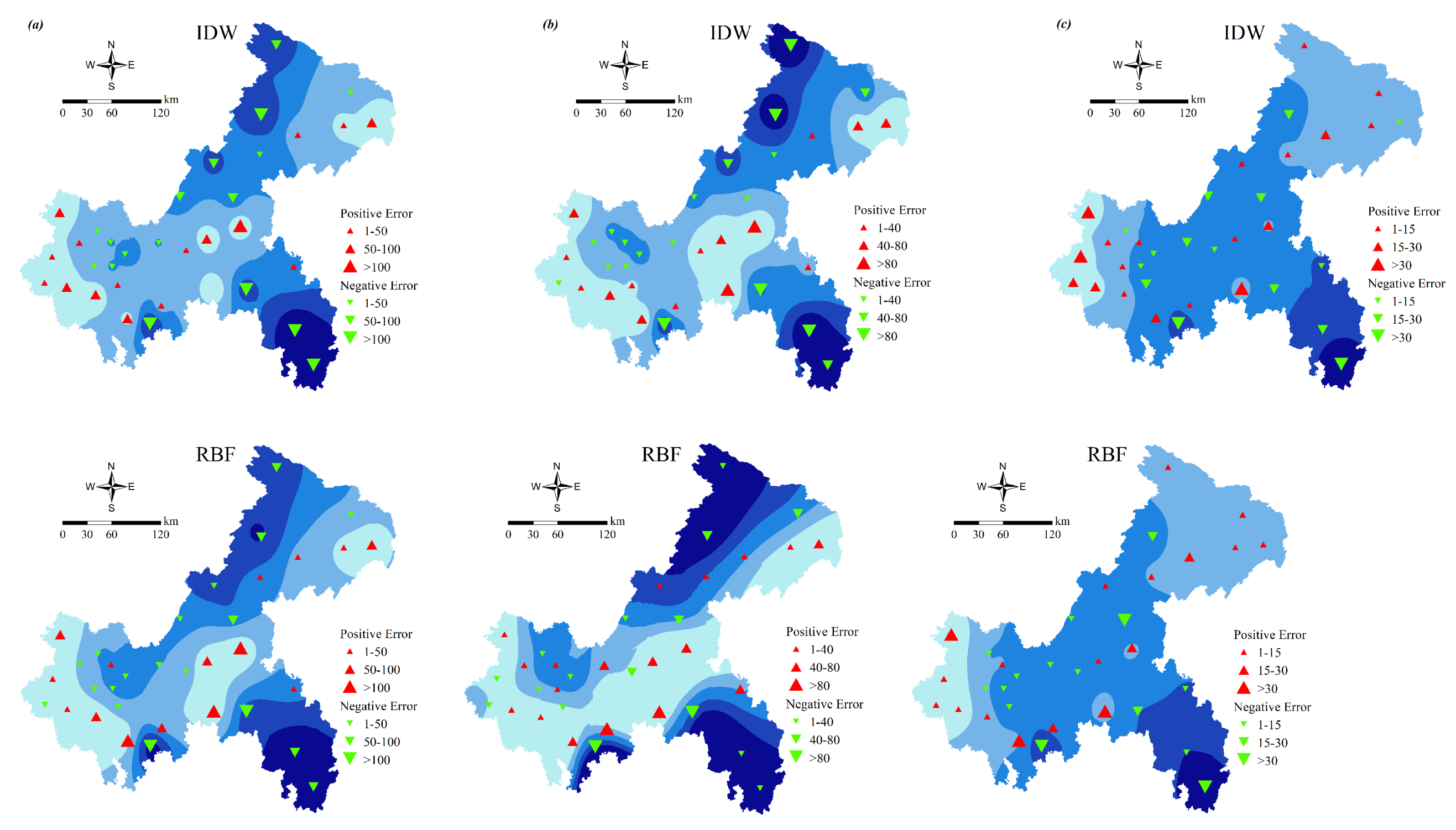
Based on the daily precipitation data from 34 meteorological stations with a time span of 1991–2019, six spatial interpolation techniques including deterministic (IDW, RBF, DIB, KIB) and geostatistical (OK, EBK) interpolation were applied to the mean annual precipitation, rainy-season precipitation and dry-season precipitation patterns in Chongqing city to generate continuous precipitation surfaces within GIS environment, and spatial variability maps of three rainfall scenarios are shown in Figure 3.
The colored dividing lines in Figure 3 are precipitation contours. Statistical analysis shows that approximately 75% of annual precipitation in Chongqing is concentrated in the rainy season (May–October), while approximately 25% is distributed in dry season (November–April). The intra-annual distribution of precipitation is extremely uneven, manifesting significant seasonal differences. Spatially, the western and central regions are low-value precipitation areas, followed by the northeastern areas. The southeastern region is the area of high precipitation values, followed by parts of the northwestern region. The spatial and temporal distribution of precipitation in Chongqing is inhomogeneous.

4.2. Performance of Different Spatial Interpolation Methods

Comparison of Interpolation Methods under Different Climatic Conditions

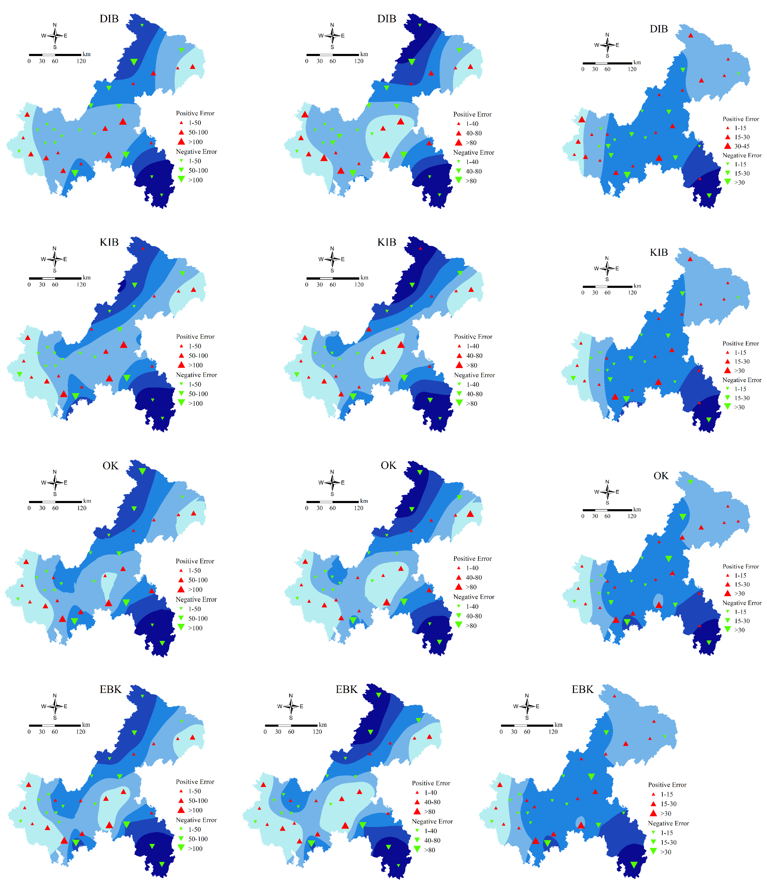
For the sake of visualizing the error distribution in different spatial interpolation methods in replicating varying rainfall magnitudes, error degree in each meteorological station from each method is drawn based on the corresponding spatial distribution maps of precipitation, which are given in Figure 4. Among them, a positive error means that the interpolator overestimates precipitation and is marked in red; a negative error represents an underestimate which is marked in green. The relative size of the marked graph represented the relative size of the error value.
As shown in Figure 4, it is evident that some interpolation methods estimated high errors, most notably IDW, indicating that the accuracy of this method is relatively low and not applicable to the study area. In general, a high degree of positive errors is observed in the low-precipitation areas, while negative errors are mostly observed in the high-precipitation areas, which indicates to some extent that the interpolation methods are mostly close to the average of the observed values for the estimation of the areas with unhomogeneous precipitation.
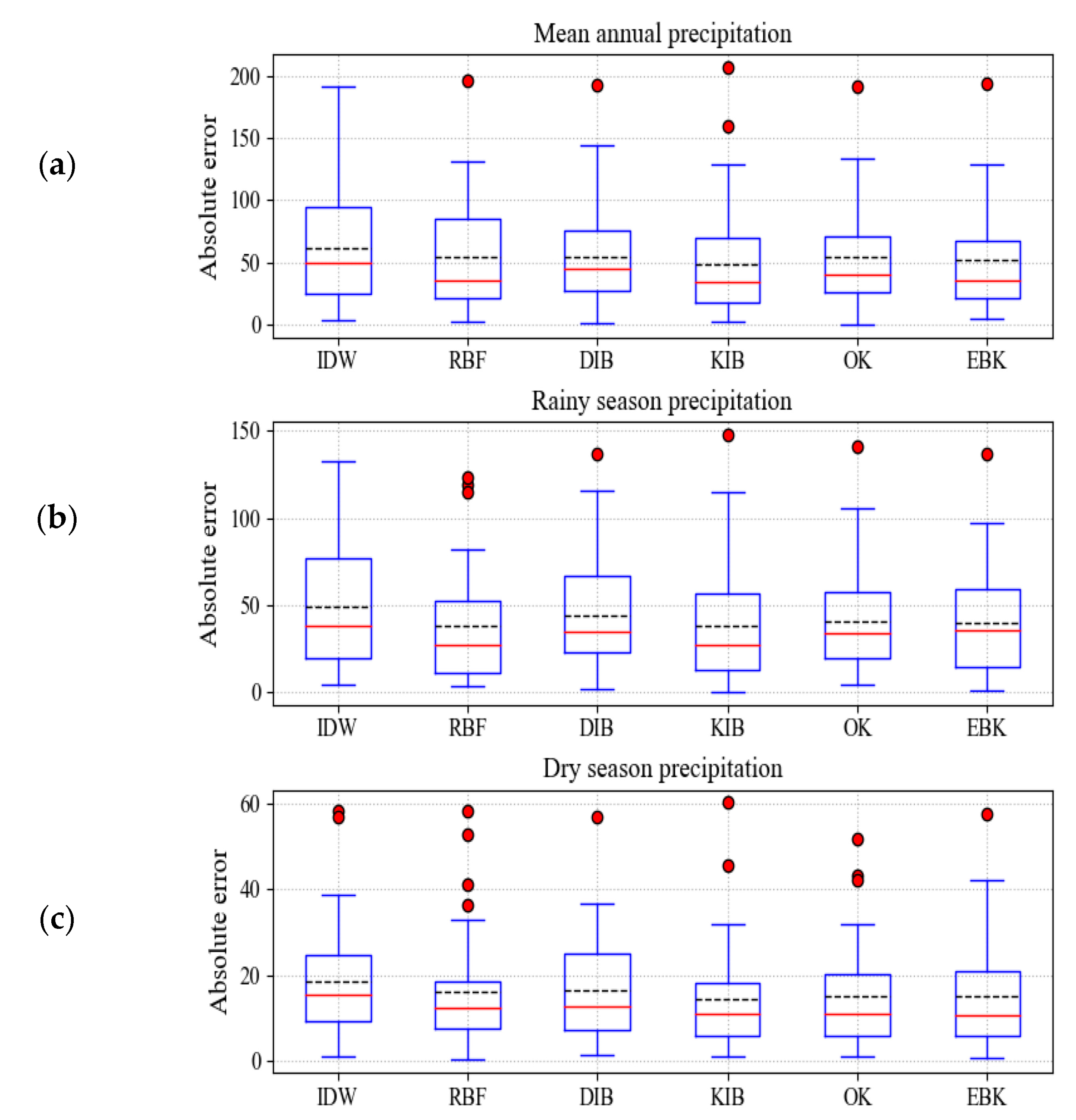
To further figure out the performance of six interpolation methods in replicating rainfall magnitudes under different climatic conditions, the absolute error distributions of different methods are presented as box plots in Figure 5. Red lines inside the box represent the median value of the absolute errors. Black dotted lines display the mean value. Red dots indicate outliers. The center represents the middle 50%, or 50th percentile, of the data set and was derived using the lower and upper quartile values [11]. The upper and lower whiskers of each box are drawn to the 90th and 10th percentiles [6], and the upper and lower edges of the rectangle (i.e., box) are defined as the 75th and 25th percentile of the data set, respectively [5,46].
Since the mean values are influenced by the outliers [11], the median (red line) is mainly considered here. Overall, among the six interpolation methods, the IDW, RBF, and DIB methods exhibit relatively high absolute errors in estimating the spatial patterns of precipitation; in particular, the IDW KIB, OK, and EBK methods have relatively low absolute errors of estimated values, which to some extent reflects the performance of the methods. The absolute errors estimated by all methods have outliers, indicating that the interpolator’s estimates of precipitation at some points differ significantly from the observed values. The absolute errors of the six methods for estimating the average annual precipitation ranged from 0.44 mm (OK method) to 207.23 mm (KIB method); the absolute errors for estimating the rainfall ranged from 0.12 mm (KIB method) to 147.68 mm (KIB method); and the absolute errors for estimating the dry-season precipitation ranged from 0.25 mm (RBF method) to 60.21 mm (KIB method).

4.3. The Error and Correlation Analysis

Based on leave-one-out cross-validation, four error measures, i.e., MSE, MAE, MAPE, SMAPE, and one accuracy measure, i.e., NSE, were adopted to examine the efficiency of each interpolation model in replicating varying rainfall magnitudes. MSE and MAE reflected the magnitude of estimation error. MAPE normalized the point error to decrease the influence of absolute error caused by outliers. SMAPE modified MAPE deficiency such that the calculations were oversize due to the tiny individual observation values. The calculation results of cross-validation are shown in Table 1.
As shown in Table 1, it is significant that the estimation accuracy of interpolation methods under different climatic conditions had remarkable distinction, the efficiencies were generally low when the rainfall magnitude was relatively high, whereas the efficiencies were relatively high when the rainfall magnitude was relative low. The interpolating accuracy increased universally with the decreased of rainfall magnitudes, further illustrating that spatial interpolators have better estimation performance in lower precipitation periods than high-value period.
Regarding comparisons among spatial interpolation methods, the optimal values of each evaluation index for each rainfall scenario are visualized. The better interpolation methods for estimating the mean annual precipitation are KIB and EBK. For the estimation in the rainy season, RBF and EBK achieve superior results. For estimating precipitation in the dry season, the KIB method achieves the best interpolation result with the optimal values of all five evaluation indicators. Hence, even with the same model, the interpolating performances were dissimilar under different climatic conditions. By contrasting the assessment indexes of six interpolation methods under the identical rainfall magnitudes, its evident that four error indexes (MSE, MAE, MAPE, SMAPE) of IDW are the maximum, and accuracy index (NSE) is the minimum. Thus, IDW has the relative worst performance in estimating the spatial distribution of precipitation among the six interpolation methods, and the accuracy of the obtained precipitation surface is low. Nevertheless, the method with the optimal performance under different climatic conditions is disparate, and further research in accordance with this issue is carried out in the next section.
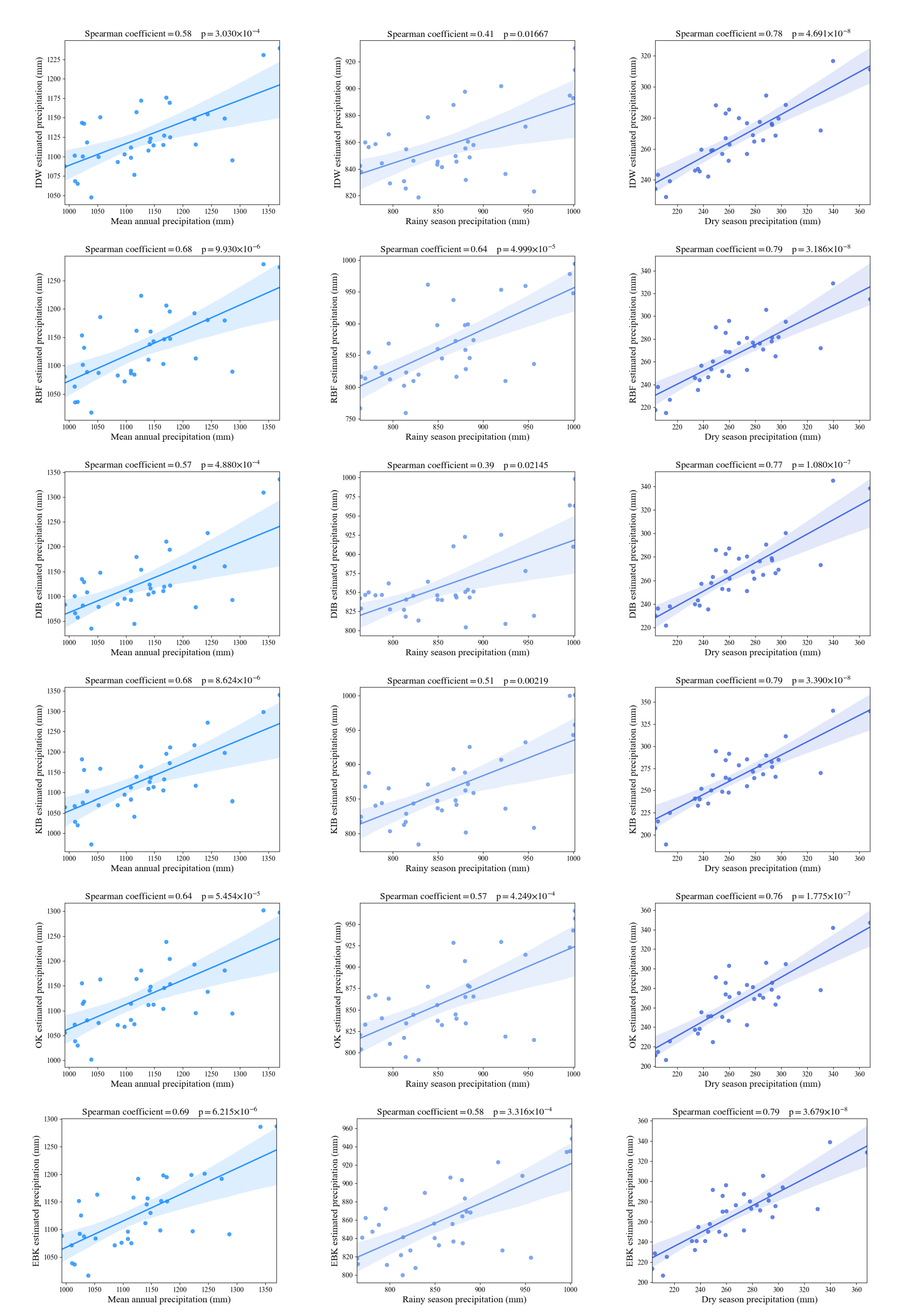
For the sake of displaying the fitting degree of the estimated and observed values, scatterplots of six interpolation methods in replicating different rainfall magnitudes are drawn in Figure 6, in which Spearman coefficients describe the correlation between the two datasets, and p-values denote significant level of correlation.
Scatterplots and correlation coefficients between the two datasets (estimated and observed values) validate the previous analysis. For each method, the Spearman coefficient is greater for the dry season than for the rainy season and annual mean precipitation patterns. The interpolation techniques have better performance in estimating the spatial distribution during periods of low precipitation. The identical method also exhibits different performances in estimating the spatial distribution under different climatic conditions, showing the uncertainty of the interpolation algorithms to some extent.
The above-mentioned results are only a separate analysis of each interpolation method under different climate conditions. To further analyze the accuracy of different interpolation methods, a comprehensive evaluation of each method based on the integrated multiple rainfall magnitudes was carried out.
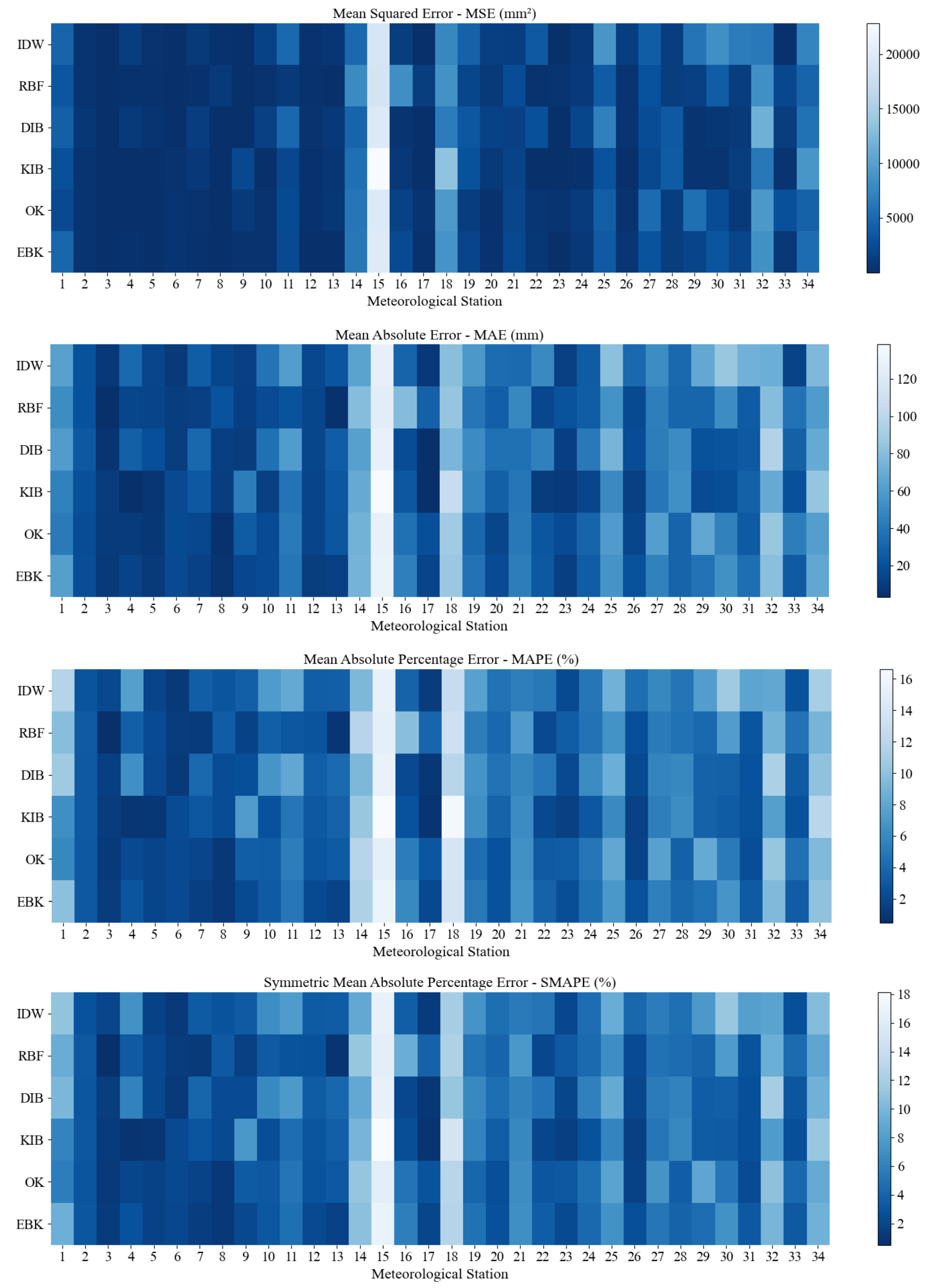
To comprehensively evaluate the effectiveness of six methods in estimating the spatial patterns under integrated multiple rainfall magnitudes, i.e., without regard to the influence of rainfall magnitude on interpolation accuracy, the estimated and observed values of 34 stations were analyzed by error measures under different climatic conditions. Four error indicators (MSE, MAE, MAPE, SMAPE) of each station in the six methods under integrated multiple rainfall magnitudes were calculated and Figure 7 was drawn for manifesting the performance of interpolation methods in estimating the spatial patterns based on integrated multiple rainfall magnitudes.
Horizontal coordinates denote 34 meteorological stations; vertical coordinates denote the six spatial interpolation methods. The values of four error indicators are distinguished in color degree—light blue indicates a larger value, dark blue indicates a smaller value. The smaller the error indicator, the better the interpolation method and the higher the accuracy in estimating the spatial patterns of precipitation. Overall, interpolation models estimate the spatial patterns of precipitation to a reasonable degree; however, outliers appear at some stations. For example, meteorological station 15 has the largest estimation error, followed by meteorological station 18. The estimation anomaly for a certain spatial location might be attributed to the complex weather variability [38] caused by the large elevation differences [45] in Chongqing, which could affect the performance of interpolation method [33].

4.4. Comprehensive Ranking by Entropy-Weighted TOPSIS

To determine the optimal method for estimating spatial precipitation patterns in Chongqing, Entropy-Weighted TOPSIS was adopted to quantize and rank the performance of six interpolation methods. Based on the performance evaluation indices (MSE, MAE, MAPE, SMAPE, NSE), the six interpolation methods are ranked in terms of their efficiency in estimating spatial patterns under different rainfall magnitudes and integrated multiple rainfall magnitudes. First, the indicators are standardized, where MSE, MAE, MAPE, SMAPE are negative indices and NSE is a positive indicator. Based on weighting results of entropy method, the distance between positive and negative ideal solutions of each method is calculated to determine the comparatively proximity (C-value) to the ideal solution, and finally the C-value is ranked to qualitatively evaluate the performance of six methods in estimating the spatial pattern of precipitation in Chongqing under different climatic conditions. The calculation results of TOPSIS evaluation are shown in Table 2.
According to TOPSIS evaluation, KIB is the optimum interpolation method under the mean annual precipitation pattern, with the comparative proximity (C-value) the highest at 0.964, followed by EBK. RBF is the optimal method in the rainy-season precipitation pattern, with the C-value the highest at 0.978, followed by KIB. KIB was the optimal method in the dry-season precipitation pattern, with the C-value the highest at 1, followed by OK. IDW was the worst method in the all precipitation patterns, with the C-value was the lowest to 0 without exception.
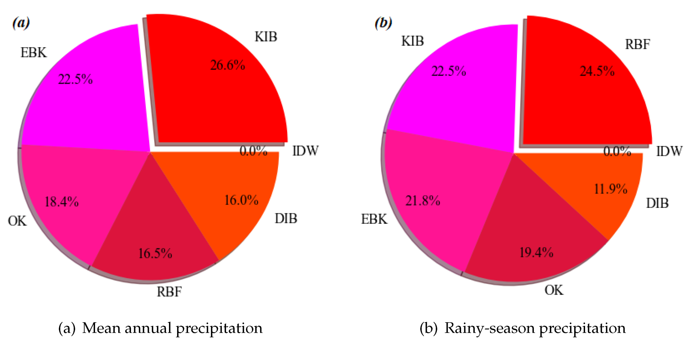
Finally, based on the C-value of the six methods under different rainfall patterns, Figure 8 maps the relative goodness of six methods in estimating the precipitation spatial pattern under different climatic conditions. The best method is marked in red. For the integrated multiple rainfall magnitudes, the C-values of six methods were mapped to one pie chart, quantitatively assessing the relative validity between the six methods for estimating precipitation spatial pattern in Chongqing.
According to Figure 8, based on integrated multiple rainfall magnitudes, KIB is the optimal model for estimating the precipitation spatial pattern in Chongqing, with the C-value is the highest to 0.954, followed by EBK. Meanwhile, IDW is the model with the lowest estimated accuracy, which is consistent with the aforementioned analysis. In addition, the rank of interpolation methods in estimating precipitation spatial pattern in Chongqing in the order of KIB > EBK > OK > RBF > DIB > IDW, the pie chart quantitatively manifests the relative effectiveness of the six methods evaluated by TOPSIS evaluation.

5. Conclusions and Discussion

This paper compared the performance of different interpolation methods (IDW, RBF, DIB, KIB, OK, EBK) in predicting the spatial distribution pattern of precipitation based on GIS technology applied to three rainfall patterns, i.e., annual mean, rainy-season, and dry-season precipitation. Multi-year averages calculated from daily precipitation data from 34 meteorological stations were used, spanning the period 1991–2019. Leave-one-out cross-validation was adopted to evaluate the estimation error and accuracy of the six methods based on different rainfall magnitudes and integrating multiple rainfall magnitudes. Entropy-Weighted TOPSIS was introduced to rank the performance of the six interpolation methods under different climatic conditions. The main conclusions can be summarized as follows.
(1) The estimation performance of six interpolation methods in the dry-season precipitation pattern is higher than that in the rainy season and annual mean precipitation pattern. Therefore, the interpolators may have higher accuracy in predicting spatial patterns for periods with low precipitation than for periods with high precipitation.
(2) Cross-validation shows that the best interpolator for annual mean precipitation pattern in Chongqing is KIB, followed by EBK. The best interpolator for rainy-season patterns is RBF, followed by KIB. The best interpolator for dry-season precipitation pattern is KIB, followed by EBK. The performance of interpolation methods replicating the precipitation spatial distribution of rainy season shows large differences, which may be attributed to the fact that summer precipitation in Chongqing is significantly influenced by western Pacific subtropical high pressure [53], low spatial autocorrelation, and the inability to perform good spatial pattern analysis using the interpolation methods. Alternatively, it can be attributed to the directional anisotropy of spatial variability in precipitation [28], or both.
(3) The Entropy-Weighted TOPSIS results show that the six interpolation methods based on integrated multiple rainfall magnitudes are ranked in order of superiority for estimating the spatial pattern of precipitation in Chongqing ordered as follows: KIB > EBK > OK > RBF > DIB > IDW. Among them, KIB is the best interpolation model for Chongqing, which can map a more accurate precipitation surface. The disadvantage is that the absolute error of estimated value relative to observed value is prone to outliers. The EBK method also has a high accuracy for estimating the spatial distribution in the region, second only to KIB. Among the six methods, IDW has the lowest interpolation accuracy and high degree of error, which is not suitable for spatial estimation of precipitation in Chongqing.
Due to the large elevation differences in Chongqing [45], the distribution of meteorological stations is uneven. Located in the eastern part of the Qinghai–Tibet Plateau, Chongqing has complex and diverse geological structures, with mountains and hills all over the territory, with obvious topographic and geomorphological features [37]. The unique topography leads to complex changes in atmospheric movements and distinct climatic characteristics [43]. However, previous research has indicated that regardless of the interpolators type, the performance of an interpolation method depends on the sample density, climatological characteristics and topography, hence there is no existing consensus about the best performance interpolation method for a local region [33]. Since the analysis of spatial events has been based on specific areas [35], our results might not be generalizable to other regions. In addition to this, this study provides an indication of the spatial distribution of accumulated rainfall in Chongqing on an annual mean, rainy-season and dry-season basis. Meanwhile, it provides some insights into the application of spatial interpolation techniques for estimating precipitation distribution and mapping continuous precipitation surface on annual and seasonal scales.

Author Contributions

Conceptualization, B.X.; methodology, B.X., R.Y.; resources and data curation, B.X.; software and visualization, R.Y.; writing—original draft preparation, R.Y.; writing—review and editing, B.X. All authors have read and agreed to the published version of the manuscript.

Funding

This research was funded by Science and Technology Research Project of Chongqing Municipal Education Commission grant number KJQN201800711.

Institutional Review Board Statement

Not applicable.

Informed Consent Statement

Not applicable.

Data Availability Statement

Meteorological data were deviled from the China Meteorological Data Service Centre (http://data.cma.cn, accessed on 28 June 2021).

Acknowledgments

The study is financially supported by the Science and Technology Research Project of Chongqing Municipal Education Commission (KJQN201800711). The authors gratefully acknowledge the editor and anonymous reviewers for their insightful and professional comments, which greatly improved this manuscript.

Conflicts of Interest

The authors declare no conflict of interest.

References

  1. Hadi, S.J.; Tombul, M. Long-term spatiotemporal trend analysis of precipitation and temperature over Turkey. Meteorol. Appl. 2018, 25, 445–455. [Google Scholar] [CrossRef] [Green Version]
  2. Hu, D.; Shu, H. Spatiotemporal interpolation of precipitation across Xinjiang, China using space-time CoKriging. J. Cent. South Univ. 2019, 26, 684–694. [Google Scholar] [CrossRef]
  3. Hadi, S.J.; Tombul, M. Comparison of Spatial Interpolation Methods of Precipitation and Temperature Using Multiple Integration Periods. J. Indian Soc. Remote Sens. 2018, 46, 1187–1199. [Google Scholar] [CrossRef]
  4. Portalés, C.; Boronat, N.; Pardo-Pascual, J.; Balaguer-Beser, A. Seasonal precipitation interpolation at the Valencia region with multivariate methods using geographic and topographic information. Int. J. Climatol. 2009, 30, 1547–1563. [Google Scholar] [CrossRef] [Green Version]
  5. Liu, D.; Zhao, Q.; Fu, D.; Guo, S.; Liu, P.; Zeng, Y. Comparison of spatial interpolation methods for the estimation of precipitation patterns at different time scales to improve the accuracy of discharge simulations. Hydrol. Res. 2020, 51, 583–601. [Google Scholar] [CrossRef]
  6. Ma, J.; Yan, X.; Hu, S.; Guo, Y. Can monthly precipitation interpolation error be reduced by adding periphery climate stations? A case study in China’s land border areas. J. Water Clim. Chang. 2017, 8, 102–113. [Google Scholar] [CrossRef]
  7. Li, H.; Wang, D.; Singh, V.; Wang, Y.; Wu, J.; Wu, J. Developing an entropy and copula-based approach for precipitation monitoring network expansion. J. Hydrol. 2021, 598, 126366. [Google Scholar] [CrossRef]
  8. Su, Y.; Zhao, C.; Wang, Y.; Ma, Z. Spatiotemporal Variations of Precipitation in China Using Surface Gauge Observations from 1961 to 2016. Atmosphere 2020, 11, 303. [Google Scholar] [CrossRef] [Green Version]
  9. Buttafuoco, G.; Conforti, M. Improving Mean Annual Precipitation Prediction Incorporating Elevation and Taking into Account Support Size. Water 2021, 13, 830. [Google Scholar] [CrossRef]
  10. Wang, S.; Huang, G.; Lin, Q.; Li, Z.; Zhang, H.; Fan, Y. Comparison of interpolation methods for estimating spatial distribution of precipitation in Ontario, Canada. Int. J. Climatol. 2014, 34, 3745–3751. [Google Scholar] [CrossRef]
  11. Cheng, M.; Yonggui, W.; Engel, B.; Zhang, W.; Peng, H.; Chen, X.; Xia, H. Performance Assessment of Spatial Interpolation of Precipitation for Hydrological Process Simulation in the Three Gorges Basin. Water 2017, 9, 838. [Google Scholar] [CrossRef] [Green Version]
  12. Zhang, X.; Liu, G.; Wang, H.; Li, X. Application of a Hybrid Interpolation Method Based on Support Vector Machine in the Precipitation Spatial Interpolation of Basins. Water 2017, 9, 760. [Google Scholar] [CrossRef] [Green Version]
  13. Srivastava, P.K.; Pradhan, R.K.; Petropoulos, G.P.; Pandey, V.; Gupta, M.; Yaduvanshi, A.; Wan Jaafar, W.Z.; Mall, R.K.; Sahai, A.K. Long-Term Trend Analysis of Precipitation and Extreme Events over Kosi River Basin in India. Water 2021, 13, 1695. [Google Scholar] [CrossRef]
  14. Dumitrescu, A.; Birsan, M.; Manea, A. Spatio-temporal interpolation of sub-daily (6 h) precipitation over Romania for the period 1975–2010. Int. J. Climatol. 2016, 36, 1331–1343. [Google Scholar] [CrossRef] [Green Version]
  15. Gajbhiye, S.; Meshram, C.; Singh, S.K.; Srivastava, P.; Islam, T. Precipitation trend analysis of Sindh River basin, India, from 102-year record (1901–2002). Atmos. Sci. Lett. 2016, 17, 71–77. [Google Scholar] [CrossRef]
  16. Bárdossy, A.; Pegram, G. Space-time conditional disaggregation of precipitation at high resolution via simulation. Water Resour. Res. 2016, 52, 920–937. [Google Scholar] [CrossRef] [Green Version]
  17. Teegavarapu, R.S.V.; Meskele, T.; Pathak, C. Geo-spatial grid-based transformations of precipitation estimates using spatial interpolation methods. Comput. Geosci. 2012, 40, 28–39. [Google Scholar] [CrossRef]
  18. Tobin, C.; Nicotina, L.; Parlange, M.; Berne, A.; Rinaldo, A. Improved interpolation of meteorological forcings for hydrologic applications in a Swiss Alpine region. J. Hydrol. 2011, 401, 77–89. [Google Scholar] [CrossRef]
  19. Bárdossy, A.; Pegram, G. Interpolation of precipitation under topographic influence at different time scales. Water Resour. Res. 2013, 49, 4545–4565. [Google Scholar] [CrossRef]
  20. da Silva, A.S.A.; Stosic, B.; Menezes, R.; Singh, V. Comparison of Interpolation Methods for Spatial Distribution of Monthly Precipitation in the State of Pernambuco, Brazil. J. Hydrol. Eng. 2019, 24, 04018068. [Google Scholar] [CrossRef]
  21. Romman, Z.A.; Al-Bakri, J.; Kuisi, M.A. Comparison of methods for filling in gaps in monthly rainfall series in arid regions. Int. J. Climatol. 2021, 1–16. [Google Scholar] [CrossRef]
  22. Alsafadi, K.; Mohammed, S.; Mokhtar, A.; Sharaf, M.; He, H. Fine-resolution precipitation mapping over Syria using local regression and spatial interpolation. Atmos. Res. 2021, 256, 105524. [Google Scholar] [CrossRef]
  23. Antal, A.; Guerreiro, P.; Cheval, S. Comparison of spatial interpolation methods for estimating the precipitation distribution in Portugal. Theor. Appl. Climatol. 2021, 145, 1193–1206. [Google Scholar] [CrossRef]
  24. Tan, J.; Xie, X.; Zuo, J.; Xing, X.; Liu, B.; Xia, Q.; Zhang, Y. Coupling Random Forest and Inverse Distance Weighting to Generate Climate Surfaces of Precipitation and Temperature with Multiple-Covariates. J. Hydrol. 2021, 598, 126270. [Google Scholar] [CrossRef]
  25. Getis, A. Spatial Pattern Analysis. In Encyclopedia of Social Measurement; k. Kempf-Leonard: New York, NY, USA, 2005; pp. 627–632. ISBN 978-0-123-69398-3. [Google Scholar] [CrossRef]
  26. Zou, W.; Yin, S.; Wang, W. Spatial interpolation of the extreme hourly precipitation at different return levels in the Haihe River basin. J. Hydrol. 2021, 598, 126273. [Google Scholar] [CrossRef]
  27. Adhikary, P.P.; Dash, C. Comparison of deterministic and stochastic methods to predict spatial variation of groundwater depth. Appl. Water Sci. 2017, 7, 339–348. [Google Scholar] [CrossRef] [Green Version]
  28. Fan, C.; Yin, S.; Chen, D. Spatial correlations of daily precipitation over mainland China. Int. J. Climatol. 2021, 1–16. [Google Scholar]
  29. Sahu, B.; Ghosh, A.K.; Seema. Deterministic and geostatistical models for predicting soil organic carbon in a 60 ha farm on Inceptisol in Varanasi, India. Geoderma Reg. 2021, 26, e00413. [Google Scholar] [CrossRef]
  30. Das, S.; Islam, A.R.M.T. Assessment of mapping of annual average rainfall in a tropical country like Bangladesh: Remotely sensed output vs. kriging estimate. Theor. Appl. Climatol. 2021, 146, 111–123. [Google Scholar] [CrossRef]
  31. Zhang, P.; Wang, Y.; Sun, H.; Qi, L.; Liu, H.; Wang, Z. Spatial variation and distribution of soil organic carbon in an urban ecosystem from high-density sampling. Catena 2021, 204, 105364. [Google Scholar] [CrossRef]
  32. Katipoğlu, O.M.; Acar, R.; Şenocak, S. Spatio-temporal analysis of meteorological and hydrological droughts in the Euphrates Basin, Turkey. Water Supply 2021, 21, 1657–1673. [Google Scholar] [CrossRef]
  33. Hurtado, S.I.; Zaninelli, P.; Agosta, E.; Ricetti, L. Infilling methods for monthly precipitation records with poor station network density in Subtropical Argentina. Atmos. Res. 2021, 254, 105482. [Google Scholar] [CrossRef]
  34. Zaghiyan, M.R.; Eslamian, S.; Gohari, A.; Ebrahimi, M.S. Temporal correction of irregular observed intervals of groundwater level series using interpolation techniques. Theor. Appl. Climatol. 2021, 145, 1027–1037. [Google Scholar] [CrossRef]
  35. Ananias, D.R.S.; Liska, G.R.; Beijo, L.A.; Liska, G.J.R.; de Menezes, F.S. The Assessment of Annual Rainfall Field by Applying Different Interpolation Methods in the State of Rio Grande do Sul, Brazil. SN Appl. Sci. 2021, 3, 687. [Google Scholar] [CrossRef]
  36. Tang, H.; Wen, T.; Shi, P.; Qu, S.; Zhao, L.; Li, Q. Analysis of Characteristics of Hydrological and Meteorological Drought Evolution in Southwest China. Water 2021, 13, 1846. [Google Scholar] [CrossRef]
  37. Guo, Q.; Liu, X.; Tang, H.; Li, Y. Prediction and correction of in situ summer precipitation in Southwest China based on a downscaling method with the BCC_CSM. Theor. Appl. Climatol. 2021, 145, 1145–1159. [Google Scholar] [CrossRef]
  38. Liu, B.; Liu, Y.; Wang, W.; Li, C. Meteorological Drought Events and Their Evolution from 1960 to 2015 Using the Daily SWAP Index in Chongqing, China. Water 2021, 13, 1887. [Google Scholar] [CrossRef]
  39. Chen, P. Effects of the entropy weight on TOPSIS. Expert Syst. Appl. 2021, 168, 114186. [Google Scholar] [CrossRef]
  40. Li, H.; Huang, J.; Hu, Y.; Wang, S.; Liu, J.; Yang, L. A new TMY generation method based on the entropy-based TOPSIS theory for different climatic zones in China. Energy 2021, 231, 120723. [Google Scholar] [CrossRef]
  41. Jiang, R.; Ci, S.; Liu, D.; Cheng, X.; Pan, Z. A Hybrid Multi-Objective Optimization Method Based on NSGA-II Algorithm and Entropy Weighted TOPSIS for Lightweight Design of Dump Truck Carriage. Machines 2021, 9, 156. [Google Scholar] [CrossRef]
  42. Chen, Y.; Li, J.; Chen, A. Does high risk mean high loss: Evidence from flood disaster in southern China. Sci. Total Environ. 2021, 785, 147127. [Google Scholar] [CrossRef] [PubMed]
  43. Xiang, B.; Zhou, J.; Li, Y. Asymmetric relationships between El Niño/La Niña and floods/droughts in the following summer over Chongqing, China. Atmos. Ocean. Sci. Lett. 2020, 13, 1–8. [Google Scholar] [CrossRef] [Green Version]
  44. Ma, Y.; Wen, T.; Xing, D.; Zhang, Y. Associations between floods and bacillary dysentery cases in main urban areas of Chongqing, China, 2005–2016: A retrospective study. Environ. Health Prev. Med. 2021, 26, 49. [Google Scholar] [CrossRef] [PubMed]
  45. Cai, S.; Fan, J.; Yang, W. Flooding Risk Assessment and Analysis Based on GIS and the TFN-AHP Method: A Case Study of Chongqing, China. Atmosphere 2021, 12, 623. [Google Scholar] [CrossRef]
  46. Célicourt, P.; Gumière, S.; Lafond, J.; Gumiere, T.; Gallichand, J.; Rousseau, A. Automated Mapping of Water Table for Cranberry Subirrigation Management: Comparison of Three Spatial Interpolation Methods. Water 2020, 12, 3322. [Google Scholar] [CrossRef]
  47. Webster, R.; Oliver, M.A. Geostatistics for Environmental Scientists, 2nd ed.; Wiley: Hoboken, NJ, USA, 2007; pp. 47–76. ISBN 978-0-470-02858-2. [Google Scholar] [CrossRef] [Green Version]
  48. Schuenemeyer, J.H.; Drew, L.J. Statistics for Earth and Environmental Scientists; John Wiley & Sons, Ltd.: Hoboken, NJ, USA, 2010; pp. 193–241. ISBN 978-1-118-10221-3. [Google Scholar] [CrossRef]
  49. Ferreira, R.G.; da Silva, D.D.; Elesbon, A.A.A.; dos Santos, G.R.; Veloso, G.; Fraga, M.D.S.; Fernandes-Filho, E.I. Geostatistical modeling and traditional approaches for streamflow regionalization in a Brazilian Southeast watershed. J. South Am. Earth Sci. 2021, 108, 103355. [Google Scholar] [CrossRef]
  50. Krivoruchko, K.; Gribov, A. Pragmatic Bayesian Kriging for Non-Stationary and Moderately Non-Gaussian Data. In Mathematics of Planet Earth; Springer: Berlin/Heidelberg, Germany, 2014; pp. 61–64. ISBN 978-3-642-32408-6. [Google Scholar] [CrossRef]
  51. Li, M.; Sun, H.; Singh, V.; Zhou, Y.; Ma, M. Agricultural Water Resources Management Using Maximum Entropy and Entropy-Weight-Based TOPSIS Methods. Entropy 2019, 21, 364. [Google Scholar] [CrossRef] [Green Version]
  52. Liu, E.; Wang, Y.; Chen, W.; Chen, W.; Ning, S. Evaluating the transformation of China’s resource-based cities: An integrated sequential weight and TOPSIS approach. Soc. Econ. Plan. Sci. 2021, 77, 101022. [Google Scholar] [CrossRef]
  53. Xiang, B.; Zeng, C.; Dong, X.; Wang, J. The Application of a Decision Tree and Stochastic Forest Model in Summer Precipitation Prediction in Chongqing. Atmosphere 2020, 11, 508. [Google Scholar] [CrossRef]
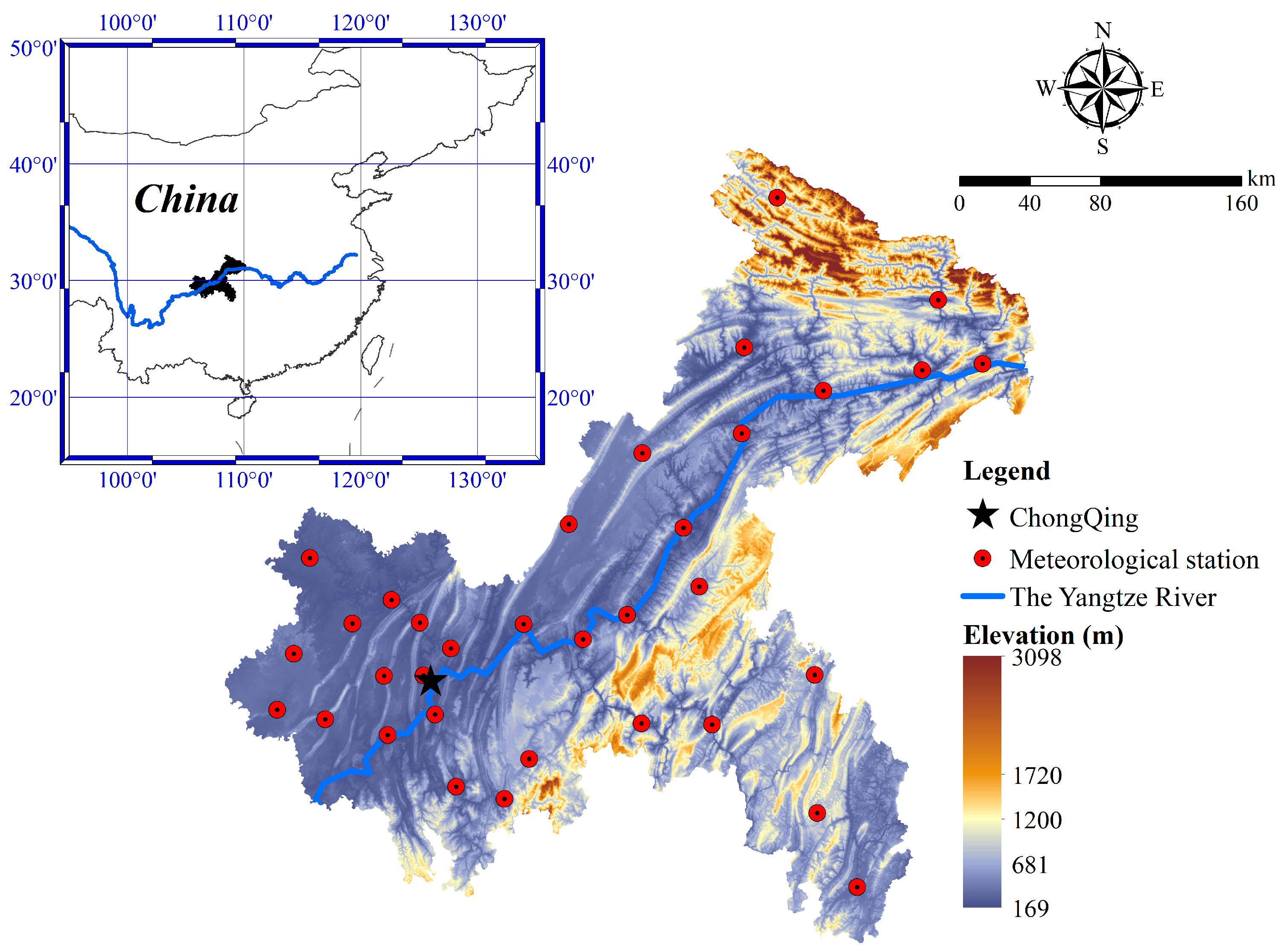
Figure 1. Geographical location and distribution of meteorological stations in Chongqing.
Atmosphere 12 01318 g001
Figure 2. Monthly mean rainfall spanning from 1991 to 2019 and the difference between rainy and dry season in accumulated rainfall.
Atmosphere 12 01318 g002
Figure 3. Precipitation spatial patterns in Chongqing under different climatic conditions based on six interpolation methods (IDW, RBF, DIB, KIB, OK, EBK): (a) mean annual; (b) rainy season; and (c) dry season.
Atmosphere 12 01318 g003aAtmosphere 12 01318 g003b
Figure 4. Spatial distribution of estimated errors under different climatic conditions based on six interpolation methods (IDW, RBF, DIB, KIB, OK, EBK): (a) mean annual; (b) rainy season; and (c) dry season.
Atmosphere 12 01318 g004aAtmosphere 12 01318 g004b
Figure 5. Boxplots of absolute errors in estimating precipitation by six interpolation methods under different climatic conditions: (a) mean annual; (b) rainy season; and (c) dry-season precipitation. Units are calculated in millimeters.
Atmosphere 12 01318 g005
Figure 6. Correlation test and Spearman coefficients between estimated and observed values based on six interpolation methods (IDW, RBF, DIB, KIB, OK, EBK): (a) mean annual; (b) rainy season; and (c) dry season.
Atmosphere 12 01318 g006
Figure 7. Cross-validation error indicators values (MSE, MAE, MAPE, SMAPE) of six interpolation methods based on integrated multiple rainfall magnitudes.
Atmosphere 12 01318 g007
Figure 8. Relative goodness of six methods based on both different rainfall magnitudes and integrated multiple rainfall magnitudes.
Atmosphere 12 01318 g008aAtmosphere 12 01318 g008b
Table 1. Assessment of interpolation models based on cross-validation error and accuracy measures under different climatic conditions. Optimal values of each assessment indicator are shown in bold.
2]*Data SetEstimationMSEMAEMAPESMAPE2]*NSE
Method(mm 2 )(mm)(%)(%)
IDW5782.7961.175.375.380.37
RBF4898.5354.444.814.780.47
MeanDIB4826.7154.704.864.870.48
AnnualKIB4545.9449.014.384.360.51
OK4698.0254.254.784.790.49
EBK4429.4551.704.584.570.52
IDW3525.0948.695.605.620.29
RBF2562.3138.054.444.420.48
RainyDIB2970.4143.925.125.120.40
SeasonKIB2704.4138.294.514.490.46
OK2651.5240.994.764.760.47
EBK2543.7939.854.634.620.49
IDW519.0518.356.906.840.61
RBF454.3116.236.005.960.66
DryDIB411.3216.286.176.130.69
SeasonKIB371.4614.505.385.390.72
OK390.9315.155.615.600.71
EBK400.9315.145.595.570.70
Table 2. TOPSIS superiority ranking of six spatial interpolation methods based on both different rainfall magnitudes and integrated multiple rainfall magnitudes. Methods with superior performance are shown in bold.
MethodPositive Distance (D)Negative Distance (D-)Comparatively Proximity (C)Sort Result
KIB0.0160.4410.9641
EBK0.0830.3740.8182
MeanOK0.1550.3110.6673
AnnualRBF0.180.2690.64
DIB0.1910.2650.5815
IDW0.448006
RBF0.010.4420.9781
KIB0.0460.410.8992
RainyEBK0.060.4010.873
SeasonOK0.1040.3530.7734
DIB0.2380.2140.4745
IDW0.448006
KIB00.44711
OK0.0630.3860.862
DryEBK0.0730.3750.8363
SeasonDIB0.1890.270.5884
RBF0.2130.2380.5285
IDW0.447006
KIB0.0240.490.9541
EBK0.070.440.8632
IntegratedOK0.1260.3790.753
ScenarioRBF0.1270.3730.7464
DIB0.2410.2650.5245
IDW0.5006
Publisher’s Note: MDPI stays neutral with regard to jurisdictional claims in published maps and institutional affiliations.