Intercomparisons of Tropospheric Wind Velocities Measured by Multi-Frequency Wind Profilers and Rawinsonde

Abstract

Concurrent measurements of three-dimensional wind velocities made with three co-located wind profilers operated at frequencies of 52 MHz, 449 MHz, and 1.29 GHz for the period 12–16 September 2017 are compared for the first time in this study. The velocity–azimuth display (VAD) method is employed to estimate the wind velocities. The result shows that, in the absence of precipitation, the root mean square difference (RMSD) in the horizontal wind speed velocities U and wind directions D between different pairs of wind profilers are, respectively, in the range of 0.94–0.99 ms⁻¹ and 7.7–8.3°, and those of zonal wind component u and meridional wind component v are in the respective ranges of 0.91–1.02 ms⁻¹ and 1.1–1.24 ms⁻¹. However, the RMSDs between wind profilers and rawinsonde are in the range of 2.89–3.26 ms⁻¹ for horizontal wind speed velocity and 11.17–14.48° for the wind direction, which are around 2–3 factors greater than those between the wind profilers on average. In addition to the RMSDs, MDs between wind profilers and radiosonde are around one order of magnitude larger than those between wind profilers. These results show that the RMSDs, MDs, and Stdds between radars are highly consistent with each other, and they are much smaller than those between radar and rawinsonde. This therefore suggests that the wind profiler-measured horizontal wind velocities are much more reliable, precise, and accurate than the rawinsonde measurement.

Key Points:

• First comparisons of horizontal wind velocities measured by co-located wind profilers operated at VHF, UHF, and L bands;
• Comparison of horizontal wind velocities between wind profilers and rawinsonde;
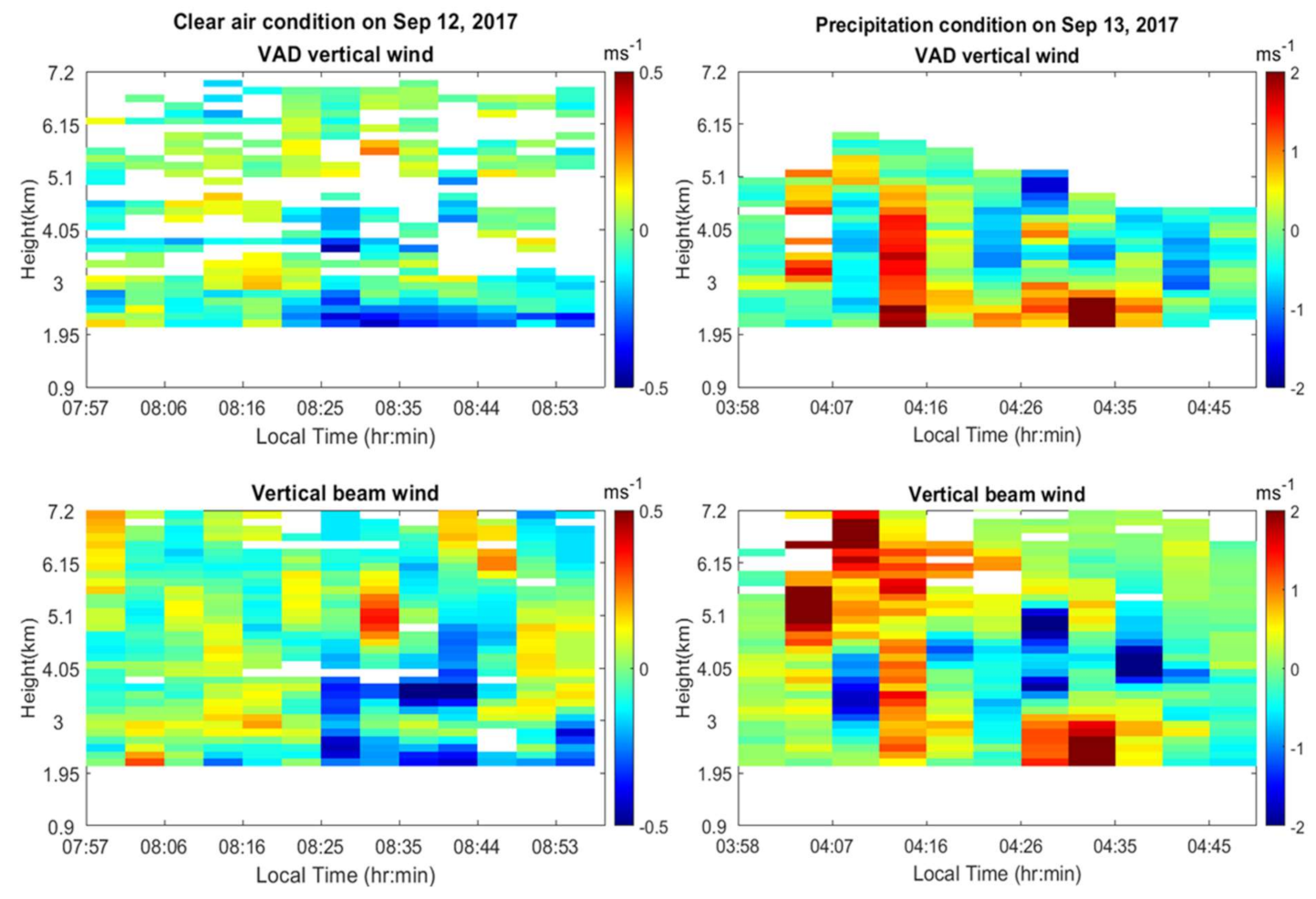
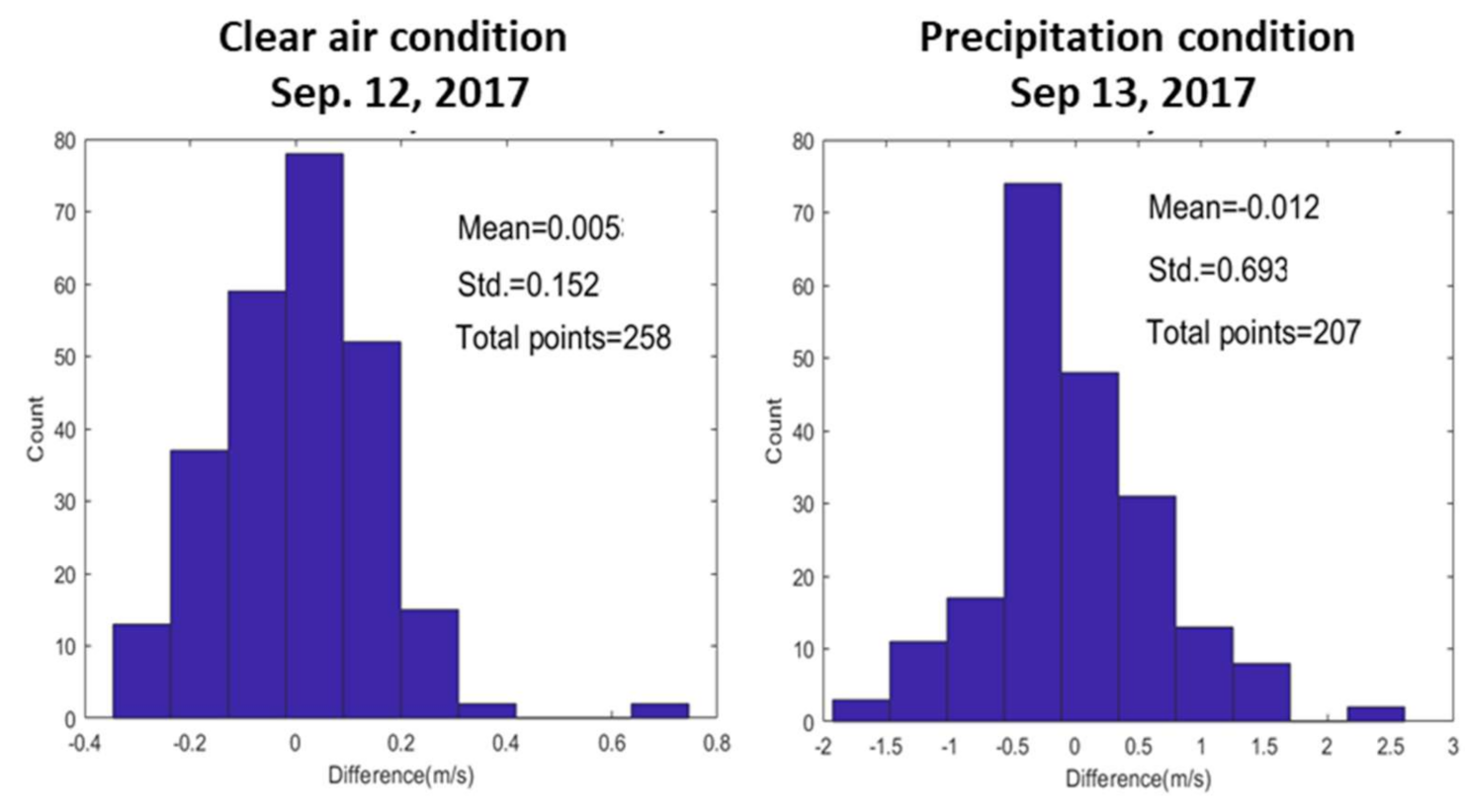
• Diagnosis of the precipitation effect on wind profiler-measured wind velocities using the VAD method.

1. Introduction

With the implementation of the coherent integration technique at the Jicamarca very-high-frequency (VHF, 30–300 MHz) radar, making it possible to measure the atmospheric wind and turbulence in the early 1970s [1], the notion of wind profiles to detect the echoes backscattered by atmospheric refractivity irregularities (or clear air turbulences) at Bragg scale exclusively for wind and turbulence measurement emerged. Since then, a number of wind profiling radars, or Mesosphere–Stratosphere–Troposphere (MST) radars, operating at different carrier frequencies from lower VHF to upper ultra-high-frequency (UHF, 0.3–3 GHz) bands, were successively developed and deployed worldwide, such as the 40 MHz Sunset and 41 MHz Urbana radars in the USA [2,3], the 53.5 MHz SOUSY radar in Germany [4], the 46.5 MHz MU radar in Japan [5,6], the 52 MHz Chung-Li radar in Taiwan [7,8], the 54 MHz Adelaide radar in Australia [9], the 45 MHz Provence and 935 MHz PROUST radars in France [10,11], the 53 MHz Gadanki radar in India [12], the 46.5 MHz Aberystwyth radar in the UK [13], and so on. To the best of the authors’ knowledge, the term “profiler” was originally used by the NOAA’s Wave Propagation Laboratory in the late 1970s and first appeared in the official documentation presented by the National Science Council [14]. The name “wind profiler” was first mentioned by [15] and has been extensively used in the atmospheric community to stress the operational application of wind profiling radar (or MST radar) since 1982 [16].

The horizontal wind velocities measured by wind profilers have long been compared with those observed by rawinsonde. In general, there are two primary methods implemented in a wind profiler to measure the wind velocity, namely the Doppler beam swing (DBS) and velocity–azimuth display (VAD) methods. For the DBS method, three-dimensional wind velocity is estimated from the Doppler (radial) velocities by steering the radar beams in the vertical and several (at least two mutually orthogonal) azimuthal directions at specific zenith angles (usually greater than 12° to avoid the underestimation of the horizontal wind velocity caused by the aspect sensitivity effect) [17], respectively. The horizontal wind velocity is estimated through combining the radial velocities observed by the oblique beams in the different directions, and the vertical wind velocity is directly measured from the vertically pointed radar beam. In general, the use of wind profilers to measure tropospheric wind with the DBS method is subject to the uncertainty of the measurement. For example, Weber and Wuertz [18] found that the standard deviation of the difference in the horizontal wind velocities between rawinsonde and a 915 MHz wind profiler is approximately 2.5 ms⁻¹. May [19] compared the hourly averaged horizontal wind measurements made with a 915 MHz wind profiler and rawinsonde for 20 months. The standard deviations of the differences between rawinsonde and profiler measurements were, respectively, around 4.6 ms⁻¹ for zonal wind velocity u and meridional wind velocity v. With the DBS method, Saïd et al. [20] compared horizontal wind velocities measured by a 1274 MHz wind profiler and co-located rawinsonde and found that the standard deviation of the wind velocity difference was approximately 1.5 ms⁻¹. However, the standard deviation will be around 2 ms⁻¹ if the separation between the wind profiler and the rawinsonde station is 61 km. Kottayil et al. [21] validated wind measurements made with a 205 MHz radar located in Cochin, India, using a nearly co-located radiosonde with a separation of 1 km between them, and the results indicated that the standard deviations of the overall wind differences for zonal and meridional components were, respectively, 1.95 and 1.56 ms⁻¹. Kim et al. [22] compared the wind fields retrieved from a UHF band wind profiler at 1290 MHz and S-band weather radars to those obtained by a numerical forecasting model as well as rawinsonde data. They showed that the root mean square errors (RMSEs) of the u and v components between model estimates and the wind profiler measurements were 3.39 ms⁻¹ and 2.58 ms⁻¹, respectively, and the RMSE of their wind velocities was 3.16 ms⁻¹. Mohanakumar et al. [23] compared horizontal wind velocities between a 205 MHz wind profiler and rawinsonde measurements and showed that they bear high correlations, with coefficients of 0.99 and 0.93 for zonal and meridional winds, respectively. The standard deviations of the radar measurements with respect to radiosonde measurements were found to be 1.85 ms⁻¹ for zonal wind and 1.66 ms⁻¹ for meridional wind.

In addition to the DBS method, numerous wind profilers operated at VHF and UHF bands measure horizontal and vertical wind velocities using the VAD method. This method uses a sinusoidal equation as a function of radial velocities and azimuth angles to best fit to the Doppler velocities that are observed by obliquely pointed radar beams in different azimuth angles at a fixed zenith angle to obtain the horizontal and vertical velocities [24]. Originally, the VAD method was first implemented in meteorological radar for horizontal wind observation. It is generally assumed that the hydrometeors are frozen in the background atmosphere and move with the horizontal wind [25]. Ishii et al. [26] employed the VAD method in a coherent Doppler lidar to estimate three-dimensional wind velocity, which was compared with the wind measurement made with a co-located VHF radar using full correlation analysis and the spaced antenna drift (SAD) method. The result indicated that the SAD-estimated horizontal wind velocities were smaller than the VAD-measured wind velocities. Strauch et al. [27] used a three-beam DBS method to estimate the precision and accuracy of a 405 MHz wind profiler. The results indicated that the standard deviation of the profiler-measured horizontal wind velocity was approximately 1.3 ms⁻¹ after vertical wind correction. Larsen [28] compared radar 1-h-averaged horizontal wind velocity measured by a 50 MHz VHF radar and rawinsonde measurement with a separation of 35 km between them and the result showed that the root-mean square errors between them were in the range of 3.21–9.3 ms⁻¹ in zonal and 4.66–12.73 ms⁻¹ in meridional components. The difference in the two may be attributed to the spatial and temporal variability of the wind velocities. Strauch et al. [29] compared wind velocities measured by 50 MHz and 405 MHz wind profilers and found that the root mean square difference (RMSD) in the horizontal wind velocities was 1.071 ms⁻¹.

Although the rawinsonde-measured horizontal wind velocity has long been employed to serve as the standard reference to assess the accuracy and precision of the wind velocity measured by wind profilers for academic research and weather/meteorological applications (e.g., [18,30]), theoretical analysis and radar experiments have shown that the precision of the rawinsonde-measured horizontal wind velocity may not be better than that of the radar measurement using the DBS method [31]. However, systematic evaluations of the precision and accuracy of the VAD-deduced wind velocities measured by wind profilers operated at different frequencies in different environments are not documented. A campaign experiment for atmospheric wind measurements made with three different wind profilers operating at 52 MHz, 449 MHz, and 1290 MHz, which were co-located on the campus of the National Central University in Taiwan, was conducted during 12–16 September 2017. In addition to mutually comparing the wind velocities observed by these three radars, the radar-measured wind velocities were also compared with the rawinsonde-measured wind velocities to realize the extent of the differences between them. To the best of the author’s knowledge, irrespective of the large amount of wind velocity comparisons that have been reported in the literature, comparisons of the concurrent measurements of wind velocities made with three different radars operating at lower VHF, lower UHF, and L bands (1–2 GHz) and co-located at the same place with a separation of less than 100 m have not been documented. This study attempts to determine the inherent uncertainty (or precision) of the wind velocities measured by three different radars, and the extent of the differences in the wind velocities measured by wind profilers and rawinsonde. In Section 2, the characteristics of different radars will be introduced, followed by methods to estimate the wind field and turbulent spectral width. In Section 3, the observational results will be presented and discussed. Conclusions will be drawn in Section 4.

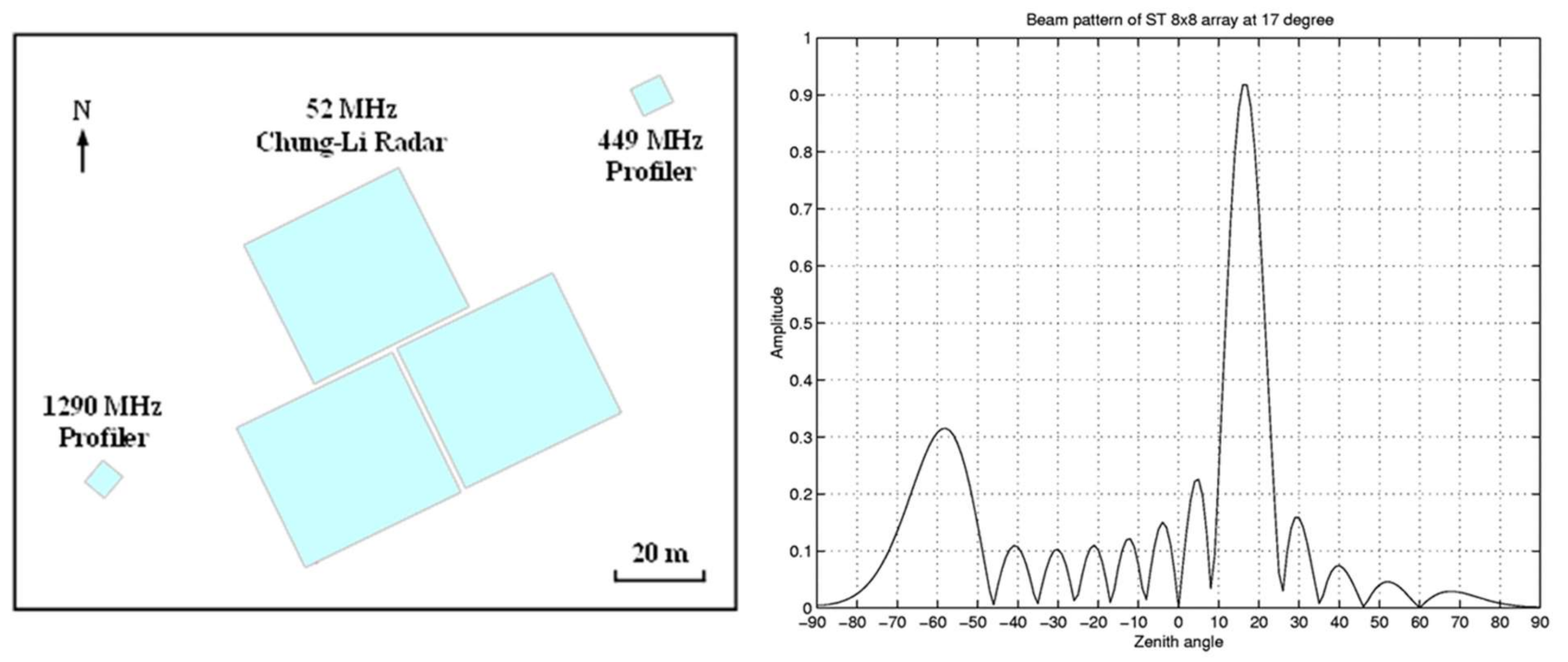
2. Experimental Setup and Data Analysis

Three co-located atmospheric radars on the campus of National Central University (24.97° N, 121.18° E) were employed in the campaign experiment for the wind velocity measurements and comparisons, i.e., 52 MHz Chung-Li VHF radar, 449 MHz wind profiler, and 1290 MHz wind profiler. The Chung-Li VHF radar is a teaching and research facility that can not only measure atmospheric wind velocity, turbulence, precipitation, lightning, meteor trail, and wave phenomena in the troposphere and/or mesosphere, but also can detect the echoes from ionospheric field-aligned irregularities at Bragg scale to study the plasma irregularities and ionospheric dynamics in the E and F regions [32,33,34,35,36]. The Chung-Li VHF radar is equipped with three phased-array antennas with a total area of 0.9 hectares; they are a strato- and troposphere (ST) array, ionospheric array, and interferometry array. A number of techniques have been developed at the Chung-Li VHF radar for wind measurement, including the DBS, VAD, spaced antenna drift (SAD), and interferometry methods. In this study, only the ST array was used in the campaign experiment. The 449 MHz wind profiler is an operational atmospheric radar that belongs to the Central Weather Bureau (CWB) and is used exclusively to routinely measure tropospheric wind velocity for weather forecasting and prediction. The antenna array of the 449 MHz wind profiler consists of 64 Yagi antenna elements arranged in an irregular configuration with nonequal separations between antenna elements. In this way, the half-power-half width of the main antenna beam is 7.6°, and the sidelobes can be suppressed (with a peak of −20 dB) to reject ground clutter, external radio interference, and aircraft clutter from nearby international airports. The 1290 MHz wind profiler is equipped with an antenna array consisting of 127 patch antenna elements with an 8° half-power-half-width main antenna beam, and it is a mobile radar that can be transported from one place to another to measure the local wind velocity for research purposes. Both the 449 MHz and 1290 MHz wind profilers were developed and manufactured by the company Radiometrics (https://radiometrics.com/; accessed on 1 September 2021). These two wind profilers have similar radar signal processing strategies and use the VAD method to measure the 3-dimensional wind velocity.

In addition to the VAD method, the 52 MHz Chung-Li VHF radar can also use the DBS method to measure 3-dimensional wind velocity. The radar parameters of the three radars that were set for the present campaign experiments are listed in

Table 1. Radar parameters of the wind profilers employed for wind comparison experiments.

Parameter	ChungLi VHF Radar	CWB UHF Radar	TTFRI L Band Radar
Frequency	52 MHz	449 MHz	1290 MHz
Radar Beam Steering
Zenith Angle	17°	14.1°	23.5°
Azimuth Angle	65.5°, 155.5°, 245.5°, 335.5°	52.6°, 112.6°, 172.6°, 232.6°, 292.6°, 352.6°	37°, 97°, 157°, 217°, 277°, 337°
Inter Pulse Period (μs)	200	32/124	76.92
Pulse Width (μs)	1	0.752/1.503	1.546
Minimum Detection Range (km)	1.65	1.01/2.59	1.57
Number of Range Gate	140	46/37	75
Number of Coherent Integration	256	16/4	16
Number of FFT	256	4096/4096	2048
Bits of Complementary Code	-	4/8	4
Number of Incoherent Integration	2	15/15	12

. Note that there were two modes (i.e., low and high modes) employed in the 449 MHz wind profiler for measuring the wind velocities in lower and higher altitude ranges. The radar parameters set for these two modes were different; they are specified and separated by a slash in the table. In order to use the VAD method to measure wind velocity, the oblique radar beams should be steered toward different azimuth angles to observe respective radial velocities for the estimation of the 3-dimentional wind velocity. The sequences of beam steering of the three radars were different. The VHF radar steered the oblique radar beams in a sequence of vertical → north → vertical → east → vertical → south → vertical → west → vertical to complete a cycle of beam steering. The UHF wind profiler steered the beams in a sequence of 52.6° → 112.6° → 172.6° → 232.6° → 292.6° → 352.6° → 52.6° for a cycle. The L-band wind profiler steered the beams in a sequence of 37° → 97° → 157° → 217° → 277° → 337° → zenith → 37° for a beam steering cycle. With the radar parameters shown in Table 1, combined with the beam steering sequence, after data analysis and processing, the time resolution of the horizontal wind velocities for the VHF radar was 5 min and that of the UHF and L-band wind profilers was 10 min.

The left-hand panel of Figure 1 shows the deployment of the antenna arrays of the three atmospheric radars at the experimental site for the wind observation campaign. As shown, the antenna array of the 52 MHz VHF radar consists of 3 square-shaped antenna modules with 64 Yagi antenna elements each, which are arranged as an isosceles triangle. Due to the grating lobe effect, there is a large grating sidelobe present in the antenna pattern of the 52 MHz VHF radar as the radar beam is steered toward an off-zenith angle of 17°, as shown in the right-hand panel of Figure 1. The grating sidelobe with a peak gain of around 9 dB weaker than the main lobe is pointed at an off-zenith angle of approximately 58° in the opposite direction to the main lobe. The radar returns received by this large grating sidelobe may cause problems in the estimation of the Doppler velocity of the clear air echoes for the wind velocity measurement, especially in a precipitation environment. Nevertheless, in the absence of vertical air velocity, it is not difficult to distinguish the sidelobe echoes from the main lobe echoes in Doppler spectral domain in accordance with the following relation for the 52 MHz VHF radar:

$$V_{rs}{R}_s=-5.235V_{rm}{R}_m$$

(1)

where R_m and R_s are, respectively, the ranges of the echoes detected by the sidelobe and main lobe at a specific height, and V_rs and V_rm are, respectively, the Doppler velocities of the echoes detected by the sidelobe and main lobe at ranges R_s and R_m, and 5.235 is the value of the ratio of tan(58°) to tan(17°). Figure 2 presents examples of the range distributions of the Doppler spectra of the clear air echoes for the north-pointed and south-pointed radar beams of the 52 MHz VHF radar for a precipitation-free environment, in which the clear air echoes received by the main lobe and sidelobe can be clearly discerned.

Once the Doppler velocities of the clear air echoes detected by the oblique main radar beams pointed at a number of specific azimuth angles are observed, the VAD method can be used to estimate the 3-dimensional velocity in accordance with the following equation:

$$V_R=V_{x}cos\beta cos\alpha +V_{y}sin\beta cos\alpha +Wsin\alpha =bcos\left(\beta -\theta \right)+a$$

(2)

where $V_R$ is the Doppler velocity observed by the oblique beam at specific azimuth angle β that is measured counterclockwise from due geographical east, $V_h$ is the horizontal wind speed velocity, $W$ is the vertical wind velocity, $\theta$ is the horizontal wind direction measured counterclockwise with respect to geographical east, $\alpha$ is the elevation angle of the oblique beam, $V_x$ is the zonal wind velocity, $V_y$ is the meridional wind velocity, b = V_h cosα, and a = W sinα. In order to derive the three-dimensional wind velocity, Equation (2) is best fitted to the observed radial velocities V_R as a function of β using the least-squares method. As a result, V_x, V_y, V_h, θ, and W can thus be obtained. It should be noted that a number of assumptions are made in the use of the VAD technique to retrieve atmospheric wind velocity, including a homogeneous and stationary wind field in the radar-illuminating volume during the beam steering period, radar returns scattered from clear air turbulence (or random fluctuations in the atmospheric refractive index), no aspect sensitivity effect on the observed Doppler spectra, and turbulences are uniformly distributed in the radar volume.

The statistical parameters used for evaluating the wind velocity comparisons are the correlation coefficient (C.C.), root mean square difference (RMSD), relative root mean square difference (RRMSD), mean of difference (MD), and standard deviation of difference (Stdd), which are defined below.

$$RMSD=\sqrt{\frac{1}{m}{\displaystyle \sum }_{i=1}^m{\left(x\left(i\right)-y\left(i\right)\right)}^2}$$

(3)

$$RRMSD=\frac{\sqrt{\frac{1}{m}{{\displaystyle \sum }}_{i=1}^m{\left(x\left(i\right)-y\left(i\right)\right)}^2}}{\frac{1}{m}{{\displaystyle \sum }}_{i=1}^{m}y\left(i\right)}$$

(4)

$$\mathrm{MD}=\frac{1}{m}{\displaystyle \sum }_{i=1}^m\left(x\left(i\right)-y\left(i\right)\right)={\mu }_x-{\mu }_y$$

(5)

$$\mathrm{Stdd}=\sqrt{\frac{1}{m}{\displaystyle \sum }_{i=1}^m{\left(\Delta x\left(i\right)-\Delta y\left(i\right)\right)}^2}$$

(6)

where μ_x and μ_y are, respectively, the mean values of x(i) and y(i), Δx(i) = x(i) − μ_x, Δy(i) = y(i) − μ_y, y(i) in Equation (4) are the 52 MHz VHF radar data or the rawinsonde data when RRMSD is calculated. A linear regression analysis is carried out to quantify the relationship between each pair of radar-measured horizontal wind velocities. Note that, in this study, RMSD is a measure of the degree of separation of the measured wind velocities between two different wind profilers or between radar and rawinsonde. RRMSD is the normalization of the RMSD by dividing it by the mean of the selected reference to avoid the effect of the magnitude of the variable (or quantity) on the RMSD. MD represents the systematic bias of the wind measurement, and Stdd represents the spreading (or uncertainty) of the wind velocity differences with respect to MD. Note that Stdd will be approximate to RMSD when MD is very small. Therefore, the smaller the RMSD, MD, and Stdd, the greater the degree of consistency between these two sets of wind velocities.

3. Results and Discussion

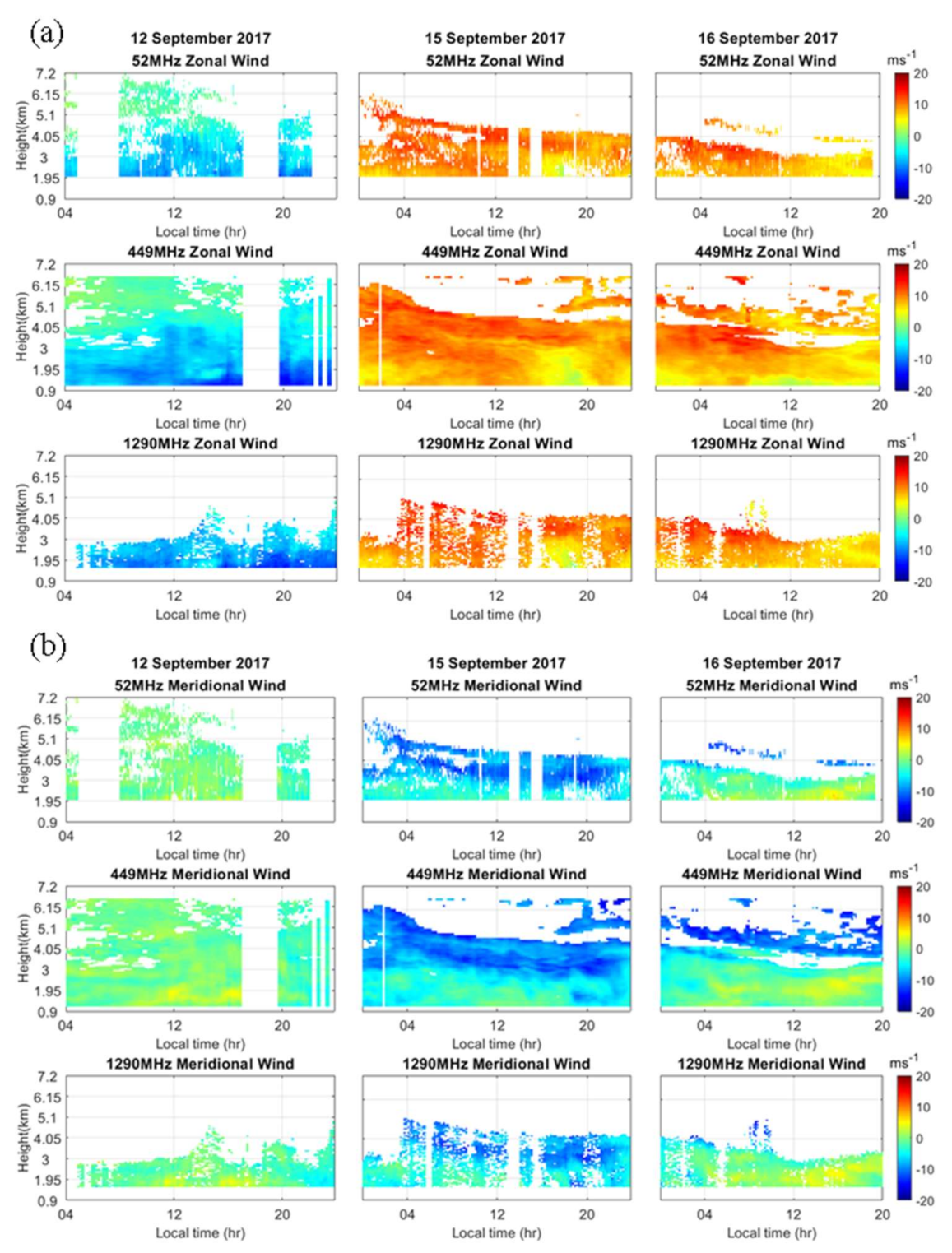
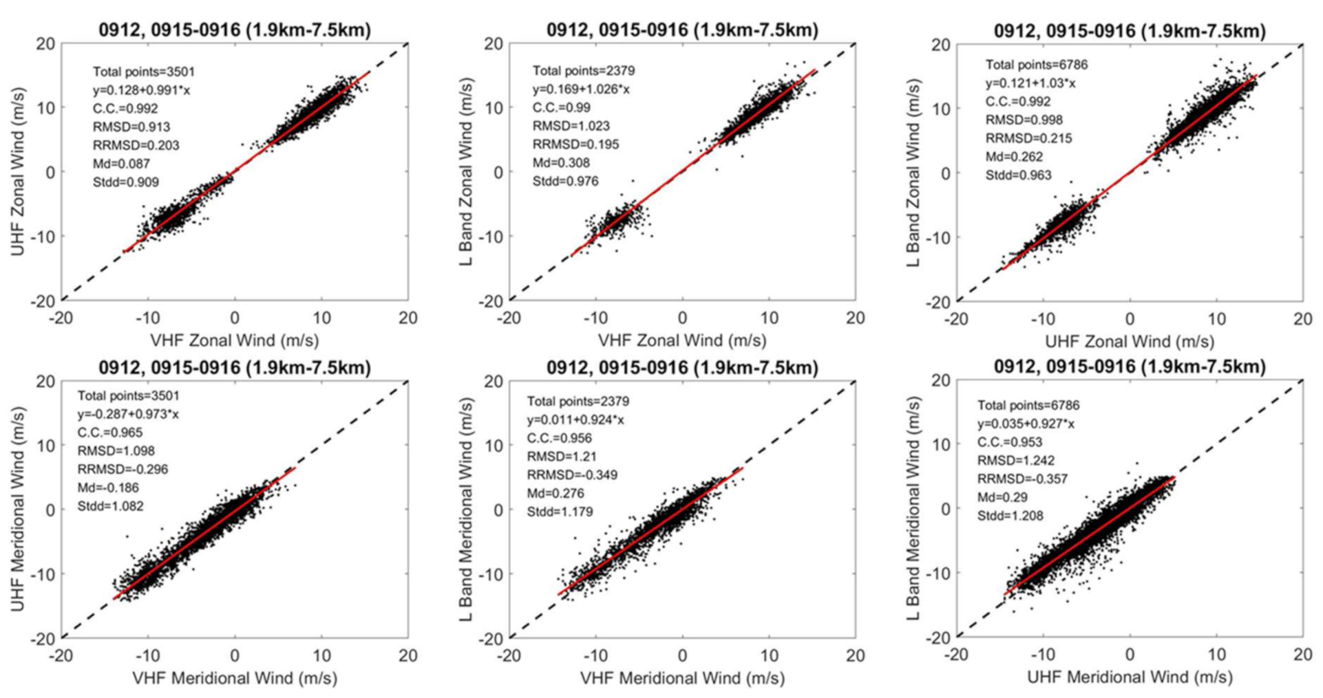
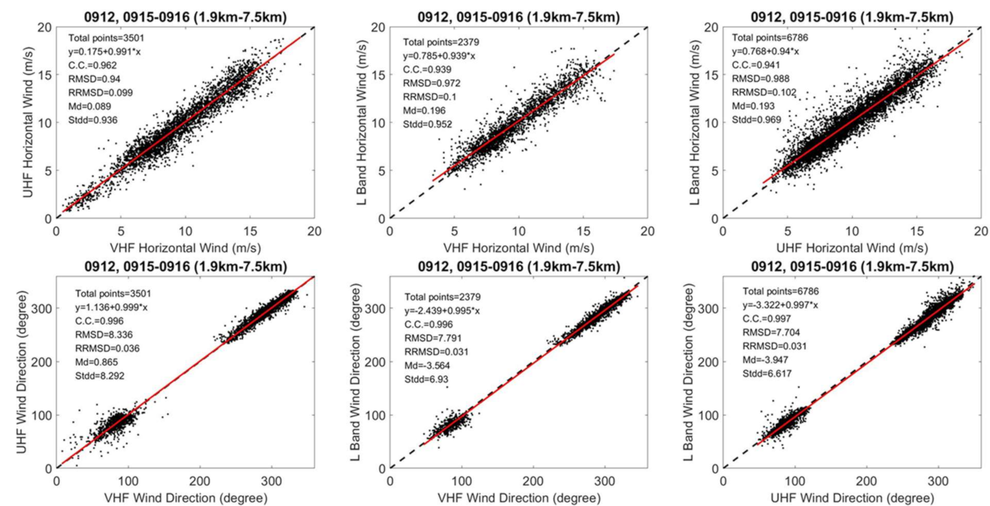
3.1. Comparisons between Radar-Measured Horizontal Winds

Figure 3a shows the height–time–intensity plots of zonal wind velocity observed by the VHF radar (top panels), UHF wind profiler (middle panels), and L-band wind profiler (bottom panels) for the data measured on 12 September, 15 September, and 16 September 2017 in an environment in the absence of precipitation, in which eastward (westward) wind was positive (negative). Figure 3b presents the height–time distributions of the radar-measured meridional wind velocities on the same days, in which northward (southward) wind was positive (negative). As shown in Figure 3, an intense westward wind prevailed in a height range below around 5 km, and a weak northeastward wind dominated above 5 km on 12 September, and the prevailing winds changed dramatically from westward-prevailing wind to southeastward throughout the height range on 15 and 16 September. This change in prevailing wind pattern was attributed to the change in the peripheral circulation of Typhoon Talim when it approached Taiwan on 14 September and made a dramatic change in its trajectory course from northwestward to northeastward at approximately 300 km northeast of Taiwan. As seen in Figure 3, the patterns of the height–time distributions of the wind velocities measured by these three wind profilers are very similar. Nevertheless, a detailed examination indicates that there still exist discrepancies in the height coverages and wind velocities between different wind profilers. Note that, due to differences in operating frequencies and radar parameters set for echo signal processing, such as pulse width, coherent integration, bit number of phase code, data points of FFT, and so on, which determine the signal-to-noise ratio (SNR) of the radar returns, there are differences in the height coverages of the wind measurements of the VHF, UHF, and L-band wind profilers. Figure 4 compares zonal (upper) and meridional (lower) wind velocities between different pairs of wind profilers observed in the absence of precipitation on 12, 15, and 16 September 2017, in which the parameters of the correlation coefficient (C.C.), root mean square difference (RMSD), relative root mean square difference (RRMSD), mean of difference (MD), and standard deviation of difference (Stdd) are defined in Equations (3)–(6), respectively.

From Table 1, we note that the height resolutions of the wind velocities measured by these three radars are different, namely 143.5 m for the VHF radar, 109.6 m for low mode and 218.2 m for high mode for the UHF radar, and 212.8 m for the L-band radar. In addition, there are time differences in the wind velocities measured by different radars. In order to ensure that the comparisons of the wind velocities are reasonable and representative, the wind velocities measured by different radars should be as close as possible to each other in time and height. In this study, the wind data are selected for comparison and statistical analysis if the time differences and height separations of the radar-measured wind velocities are within ±20 s and ±25 m, respectively.

It is obvious from Figure 4 that the correlation coefficients (C.C.) of the u and v components between different radar pairs are very high, in the respective ranges of 0.99–0.992 and 0.953–0.965. The RMSDs of the u and v components between different radar pairs are, respectively, in the ranges of 0.913–1.023 ms⁻¹ and 1.098–1.242 ms⁻¹. The MDs of the u and v components are very small, with values in the range of −0.186 to 0.308 ms⁻¹. The magnitudes of the Stdds of the u and v components among the three radar pairs are in the respective ranges of 0.909–0.976 ms⁻¹ and 1.082–1.208 ms⁻¹. Due to the very small MDs, the magnitudes of the Stdds of the u and v components are approximately 0.4–0.45%, slightly smaller than those of the RMSDs. In addition, we note that the u component bears a higher correlation than the v component, and the RMSDs and Stdds of the u component are both smaller than those of the v component. Figure 5 compares the horizontal wind velocities U (upper panels) and wind directions D (lower panels) that are both calculated from the u and v shown in Figure 4. As shown, the correlations between the horizontal wind velocities U and wind direction D are very high, in the respective ranges of 0.939–0.962 and 0.996–0.997. The ranges of the RMSDs of U and D are, respectively, 0.940–0.988 ms⁻¹ and 7.704–8.336°. The MDs of U and D are also very small, in the respective ranges of 0.089 to 0.196 ms⁻¹ and −3.947° to 0.865°, implying that there is no systematic bias in the horizontal wind measurements made with these three radars operating at very different frequencies. The Stdds of U and D are, respectively, in the ranges of 0.936–0.969 ms⁻¹ and 6.617–8.292°, which are also smaller than the RMSDs. On average, the mean RMSDs of U and D are, respectively, 0.967 ms⁻¹ and 7.944°. The mean RMSDs of the u and u components are, respectively, 0.978 and 1.183 ms⁻¹. It is clear from Figure 4 and Figure 5 that the correlations of the measured horizontal wind velocities and wind directions between different radar pairs are very high, and the magnitudes of RMSD, MD, and Stdd for different pairs of radars are small and quite consistent with each other. All of these results strongly suggest that the atmospheric horizontal wind measurements by these three different radars using the VAD method are very accurate, precise, and reliable. We summarize the values of the statistical parameters, i.e., C.C., RMSD, MD, and Stdd, of the U, D, u, and v components in

Table 2. Comparisons of zonal wind (u) and meridional wind velocity (v) between wind profilers in the absence of precipitation.

Radar	VHF-UHF	VHF-L Band	UHF-L Band
Data point	3501	2379	6786
Parameter	u/v	u/v	u/v
C.C.	0.992/0.965	0.990/0.956	0.992/0.954
RMSD (m/s)	0.913/1.098	1.023/1.210	0.998/1.242
MD (m/s)	0.087/-0.186	0.308/0.276	0.262/0.290
Stdd (m/s)	0.909/1.082	0.976/1.179	0.963/1.208

and

Table 3. Comparisons of horizontal wind velocity (U) and wind direction (D) between wind profilers in the absence of precipitation.

Radar	VHF-UHF	VHF-L Band	UHF-L Band
Data point	3501	2379	6786
Parameter	U/D	U/D	U/D
C.C.	0.962/0.996	0.939/0.996	0.941/0.997
RMSD (m/s, °)	0.940/8.336	0.972/7.791	0.988/7.704
MD (m/s, °)	0.089/0.865	0.196/−3.564	0.193/−3.974
Stdd (m/s, °)	0.936/8.292	0.953/6.930	0.969/6.617

to facilitate comparisons.

Strauch et al. [27] used the three-beam DBS method to estimate the precision and accuracy of a 405 MHz wind profiler. The results indicated that the standard deviation of the profiler-measured horizontal wind velocity was approximately 1.3 ms⁻¹ with vertical wind correction, which is significantly larger than the Stdd values of the 449 MHz and 52 MHz radar pair and of the 449 MHz and 1290 MHz radar pair for the present study by approximately 34% and 39%, respectively, as shown in Table 3. Strauch et al. [29] compared the wind velocities measured by 50 MHz and 405 MHz wind profilers and found that the RMSD of the horizontal wind velocities was 1.071 ms⁻¹ which is approximately 14% larger than that measured by the 52 MHz and 449 MHz wind profilers, as shown in Figure 5 and Table 3. On the basis of a pair of radial velocities observed by off-zenith radar beams pointed in opposite directions for the Aberystwyth VHF radar operating at 46.5 MHz, Lee et al. [37] analyzed the RMSDs of the pair of horizontal wind velocities by removing vertical wind velocities from the observed radial velocities, which were directly measured by a vertically pointed radar beam. They found that the RMSDs were between 0.8 ms⁻¹ for low wind velocities (10–15 ms⁻¹) below 5 km and 2.5 ms⁻¹ for high winds (40–45 ms⁻¹) at higher altitudes. As seen in Figure 5, the magnitudes of horizontal wind velocities for our cases are in the range of 5–17 ms⁻¹, which corresponds to the low wind velocity case defined by Lee et al. [37]. In light of the fact that the correlations of the u and v components between different radar measurements are significantly high (0.95–0.99) and their RMSDs are also very consistent with each other (0.91–1.24 ms⁻¹), it can be reasonably inferred that the RMSDs of the VHF radar-measured u and v components are comparable to those between different radar pairs. In this context, the RMSD of horizontal wind velocity related to the VHF radar measurements in the present study (approximately 0.956 ms⁻¹ on average) is essentially consistent with that obtained by Lee et al. [37].

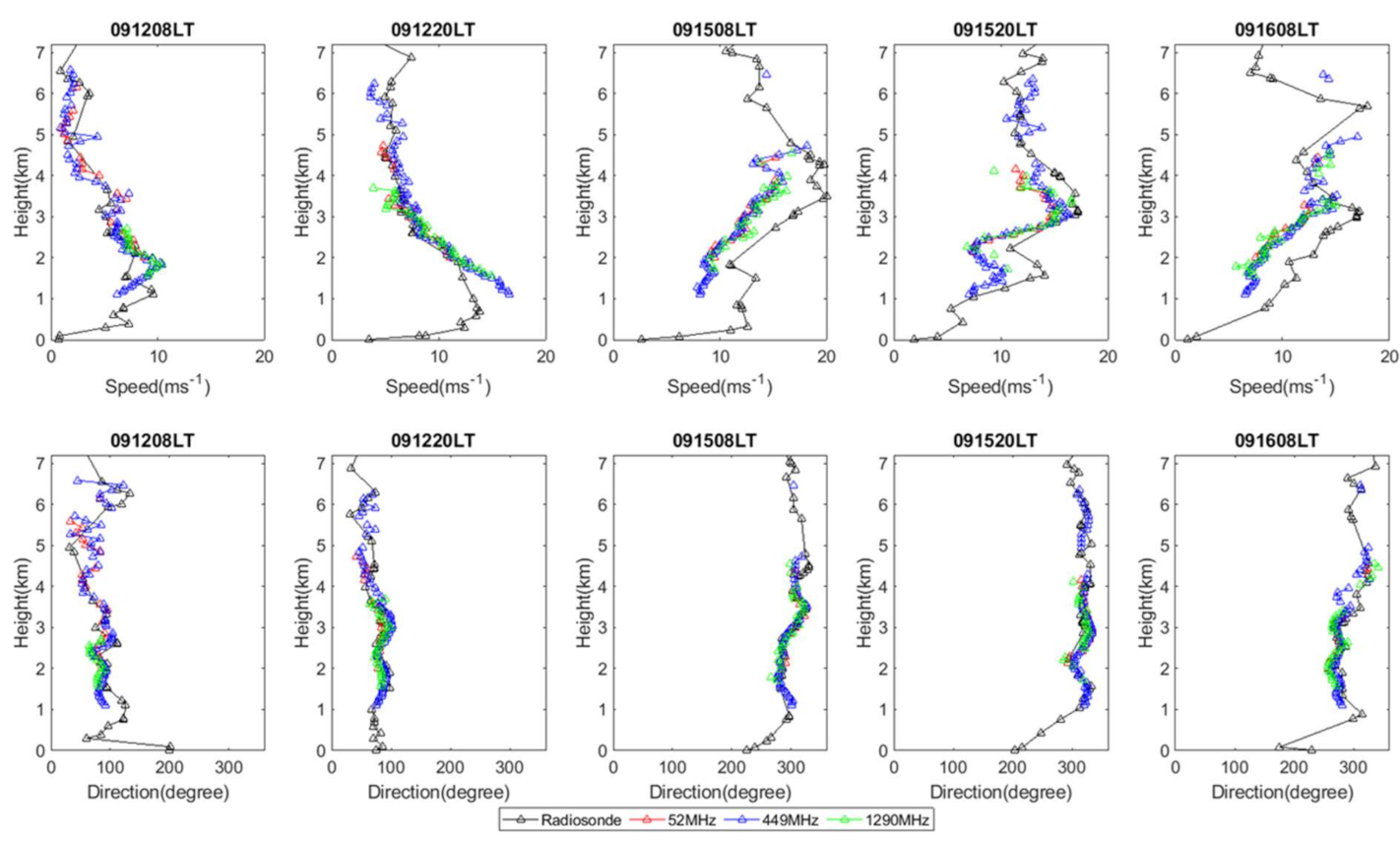
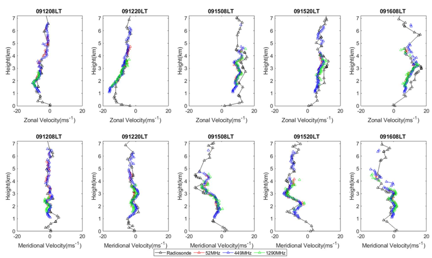
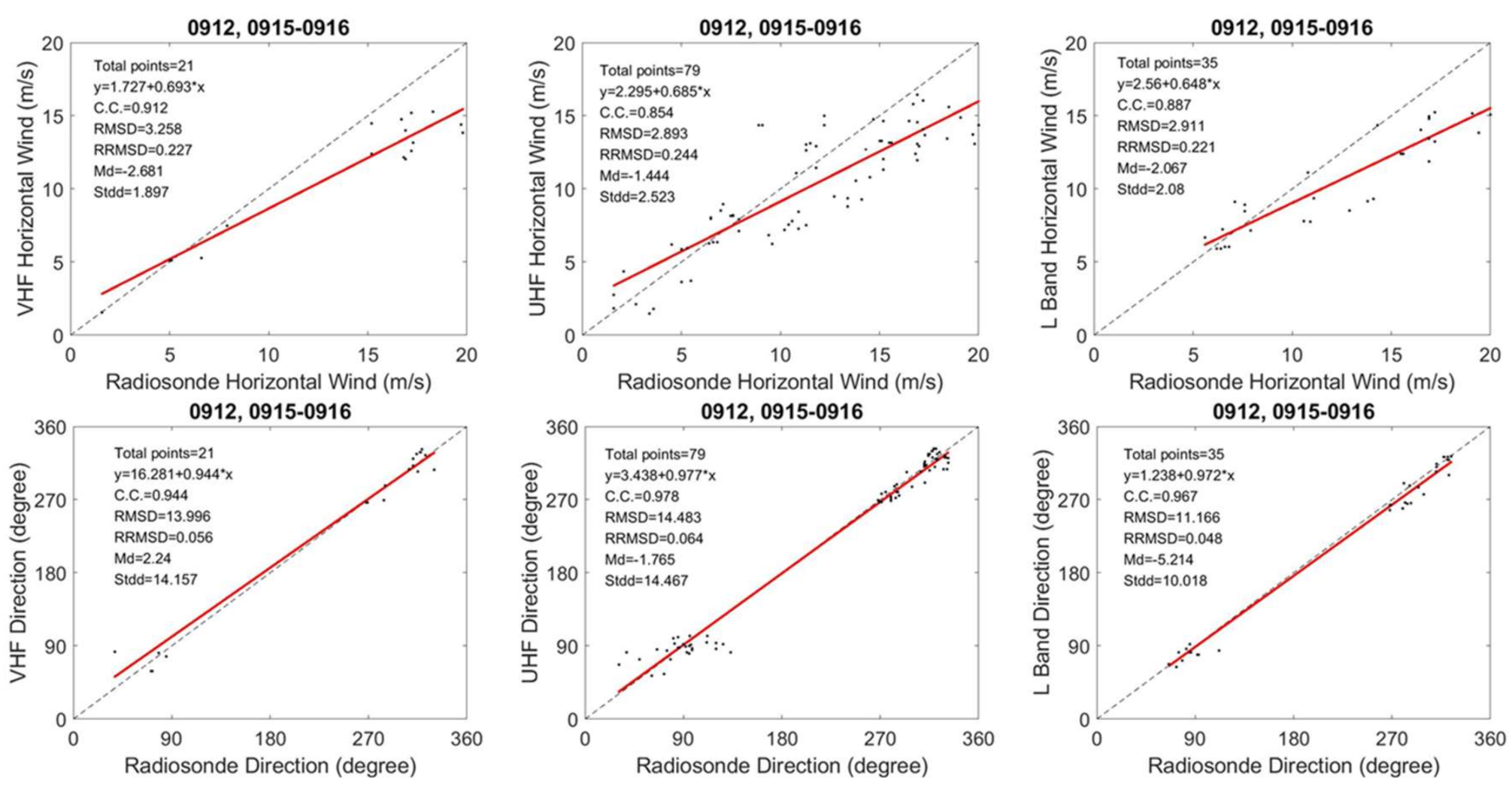
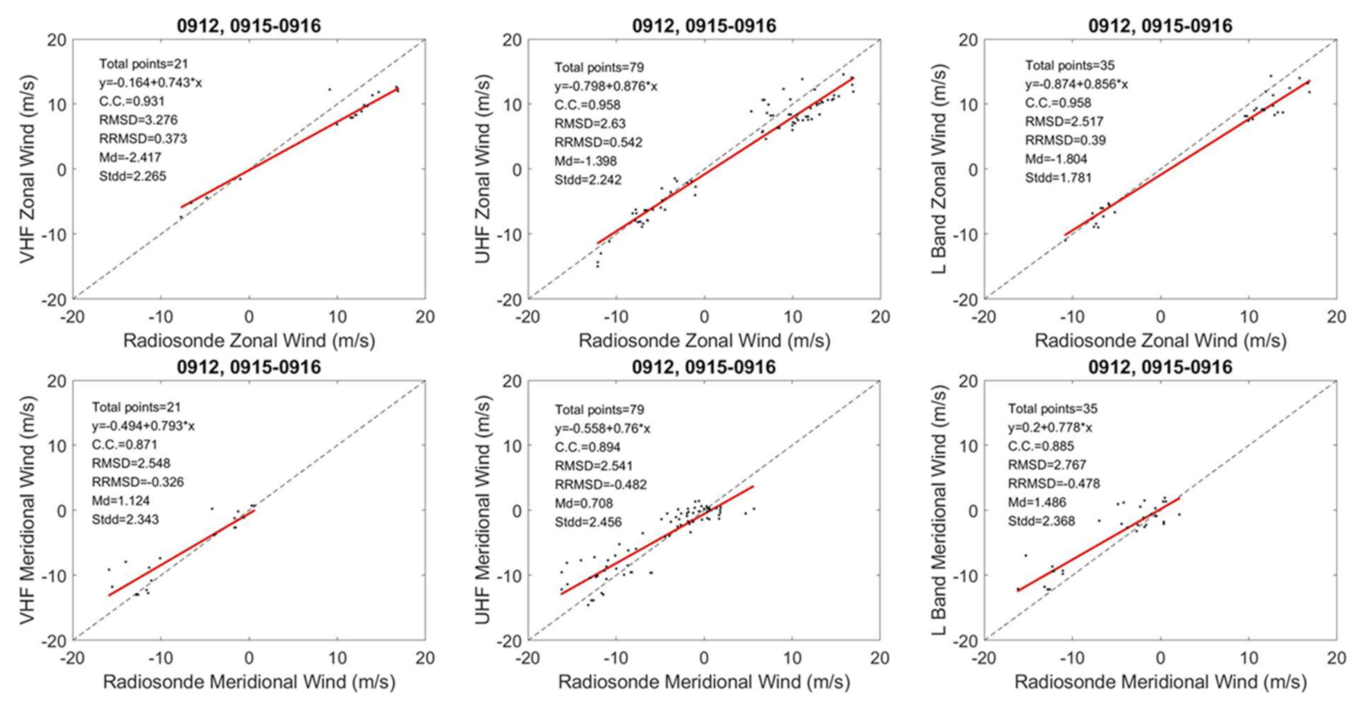
3.2. Comparisons between Radar Winds and Rawinsonde Winds

In addition to the comparisons of horizontal wind velocities between different radar pairs, as shown in Figure 4 and Figure 5, we also compare the wind velocities measured by rawinsonde (RWS) and different radars. The standard rawinsonde equipped with a global positioning system (GPS) is launched routinely at 08 and 20 LT every day at Banqiao meteorological station (24.99° N, 121.43° E) by the Central Weather Bureau, which is located at around 26 km northeast of the Chung-Li VHF radar site. Figure 6 compares the profiles of horizontal wind velocities U (upper panels) and wind directions D (bottom panels) measured by the 52 MHz radar (red curve), 449 MHz wind profiler (blue curve), 1290 MHz profiler (green curve), and rawinsonde (black curve) in the absence of precipitation. Note that the wind direction shown in Figure 6 is defined as the direction from which the wind blows, and is measured clockwise from geographical north. Namely, 0° signifies that the wind blows from north to south, and 90° means that the wind direction is westward, and so on. Figure 7 compares the profiles of the u (upper panels) and v (lower panels) components for the same data presented in Figure 6. As shown in Figure 6 and Figure 7, the radar-measured u components, v components, horizontal wind velocities, and wind directions are all in excellent agreement with one another. However, the radar-measured wind velocity profiles obtained on 15 and 16 September 2017 are not in good agreement with the rawinsonde measurements, irrespective of the good agreement between them on 12 September 2017. Quantitative analysis of the differences in the wind velocities and directions between radar and rawinsonde measurements are shown in Figure 8 and Figure 9. As shown in Figure 8, the C.C. of the u and v components between radar and rawinsonde are still high, in the respective ranges of 0.931–0.958 and 0.87–0.894. The RMSDs of the u and v components between radar and rawinsonde are, respectively, in the ranges of 2.517–3.276 ms⁻¹ and 2.541–2.767 ms⁻¹. The MDs of the u and v components are in the respective ranges of −2.418 to −1.398 ms⁻¹ and 0.708 to 1.486 ms⁻¹, and the Stdds of the u and v components are in the range of 1.781–2.266 ms⁻¹ and 2.343–2.456 ms⁻¹, respectively. Figure 9 presents scatterplots of U (upper panels) and D (lower panels) between radar and rawinsonde measurements. As shown, the correlation coefficients of U and D between radars and rawinsonde are in the respective ranges of 0.854–0.912 and 0.944–0.979. The RMSDs of U and D are, respectively, in the range of 2.893–3.258 ms⁻¹ and 11.166–14.483°. The ranges of MDs of U and D are, respectively, from −2.681 to −1.444 ms⁻¹ and from −5.214° to 2.24°, and those of Stdds of U and D are, respectively, 1.897–2.523 ms⁻¹ and 10.018–14.467°. A comparison of Figure 4, Figure 5, Figure 8 and Figure 9 shows that the correlations of the wind velocities and direction between radar measurements are higher than those between radar and rawinsonde. In addition, the RMSDs and Stdds of wind velocities and directions between radars are around 2–3 times smaller than those between radar and rawinsonde. Moreover, the magnitudes of the MDs of the wind velocities between radars are roughly one order of magnitude smaller than those between radar and rawinsonde. The statistical parameters of the wind velocities and wind directions between radars and rawinsonde measurements, i.e., C.C., RMSD, MD, and Stdd, are summarized in

Table 4. Comparisons of zonal wind (u) and meridional wind velocity (v) between wind profilers and rawinsonde (RWS).

Radar	VHF-RWS	UHF-RWS	L Band-RWS
Data point	21	79	35
Parameter	u/v	u/v	u/v
C.C.	0.931/0.872	0.958/0.894	0.958/0.885
RMSD (m/s)	3.276/2.548	2.630/2.541	2.517/2.767
MD (m/s)	−2.418/1.124	−1.398/0.708	−1.804/1.486
Stdd (m/s)	2.266/2.343	2.242/2.456	1.781/2.368

and

Table 5. Comparisons of horizontal wind velocity (U) and wind direction (D) between wind profilers and rawinsonde (RWS).

Radar	VHF-RWS	UHF-RWS	L Band-RWS
Data point	21	79	35
Parameter	U/D	U/D	U/D
C.C.	0.912/0.944	0.854/0.979	0.887/0.967
RMSD (m/s, °)	3.258/13.996	2.893/14.483	2.911/11.166
MD (m/s, °)	−2.681/2.240	−1.444/−1.765	−2.067/−5.214
Stdd (m/s, °)	1.897/14.157	2.523/14.467	2.080/10.018

to facilitate comparison.

Päschke et al. [38] compared VAD-derived horizontal wind velocities U and directions D measured by a 485 MHz wind profiler and 1.5 μm Doppler lidar for one year and found that the RMSDs of 30-min averaged U and D between them were in the respective ranges of 0.5–0.7 ms⁻¹ and 5–7°. However, RMSDs between lidar and rawinsonde measurements were 0.7–0.9 ms⁻¹ for horizontal wind velocity and 8–12° for wind direction. Note that Päschke et al. [38] applied quality control to the radar-measured wind data before intercomparisons. Nevertheless, irrespective of differences in radar frequencies and time resolutions, our results presented in Figure 5 and Table 4 show that the RMSDs of the U and D between wind profilers are comparable to those obtained by Päschke et al. [38]. However, the RMSDs between radar and rawinsonde measurements for the present results are around three-times larger for horizontal wind velocity and two-times larger for wind direction than those reported by Päschke et al. [38]. Haefele and Ruffieux [39] compared u and v components measured by a 1290 MHz wind profiler using the DBS method and rawinsonde with a time resolution of 40 min or 60 min and found that the Stdd of the u and v components between the wind profiler and rawinsonde were in the range of 1.75–2 ms⁻¹, with a correlation coefficient of 0.964 (high mode) and 0.954 (low mode). A comparison shows that their results are highly consistent with our results, as shown in Figure 9 and Table 4, although the VAD method that we use to estimate the horizontal wind velocity is very different from DBS method that they employed, and the time resolutions of our data (5 min and 10 min) are also different from those (40 min and 60 min) that they used. Rao et al. [30] compared the horizontal wind velocities measured by a 53 MHz Gadenki VHF radar with rawinsonde measurement to evaluate the performance of the DBS technique with different beam configurations in horizontal wind velocity measurement. They found that the standard deviation for a four-beam configuration varied from 1.4 to 2.5 ms⁻¹, which is very consistent with the result (1.897 ms⁻¹ for the 52 MHz VHF radar) obtained in this study.

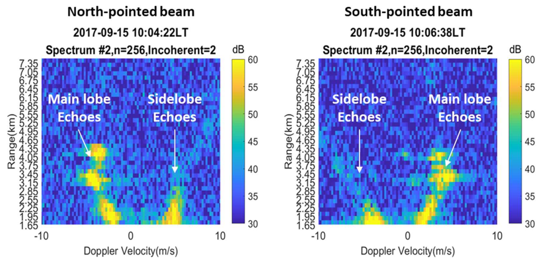
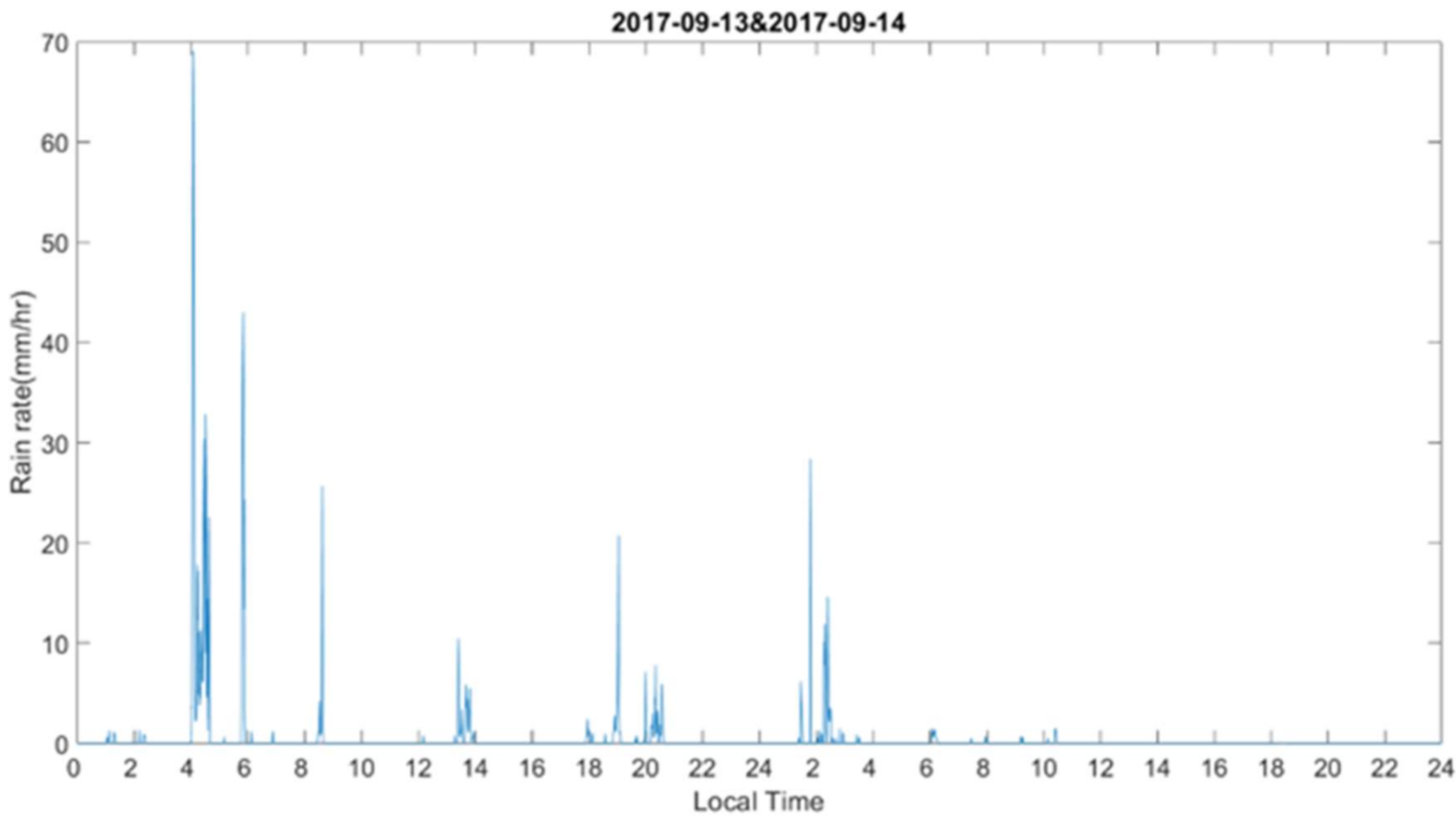
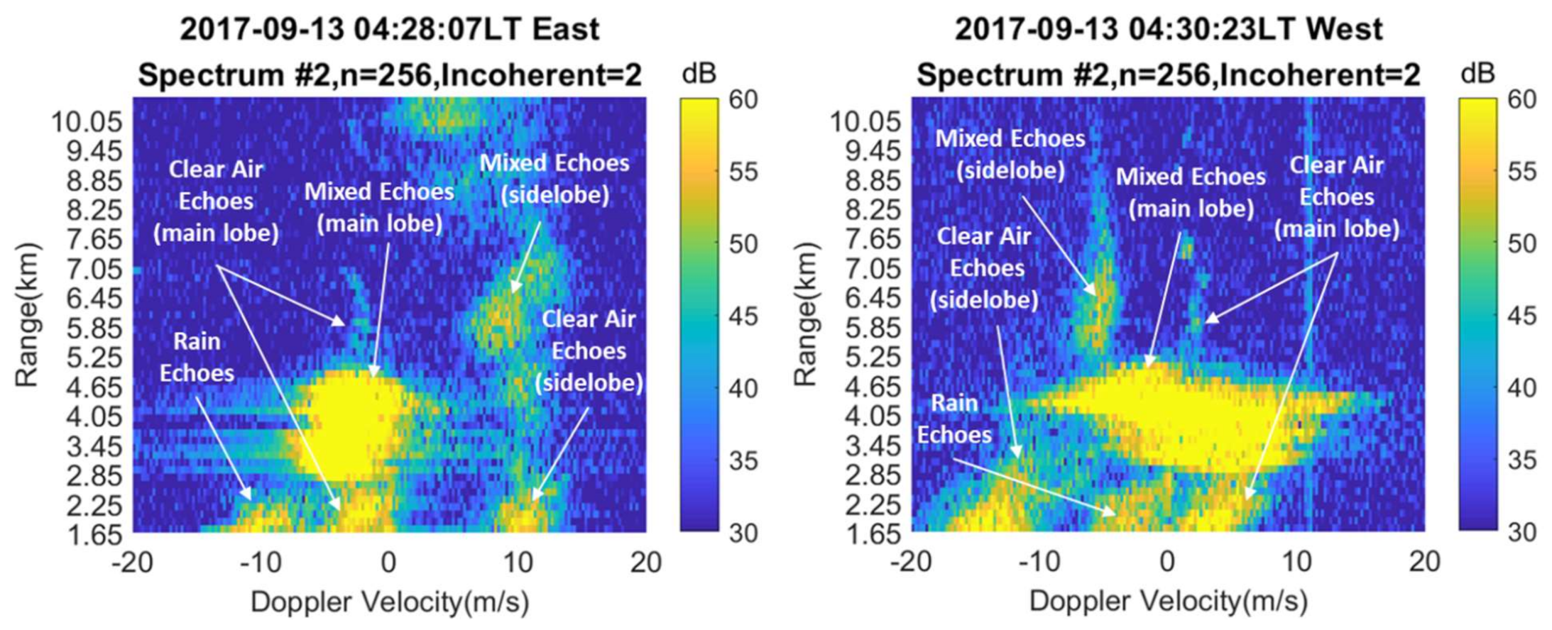
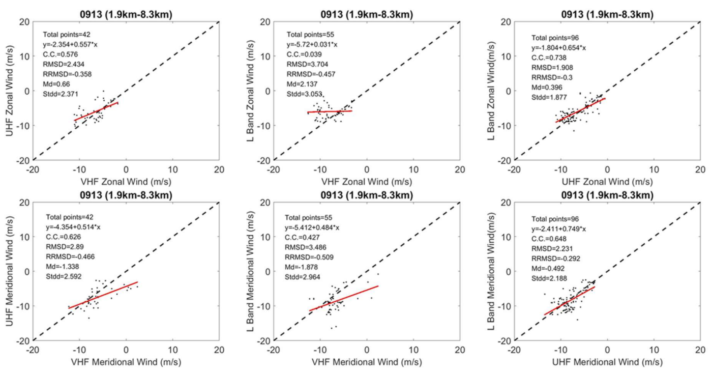
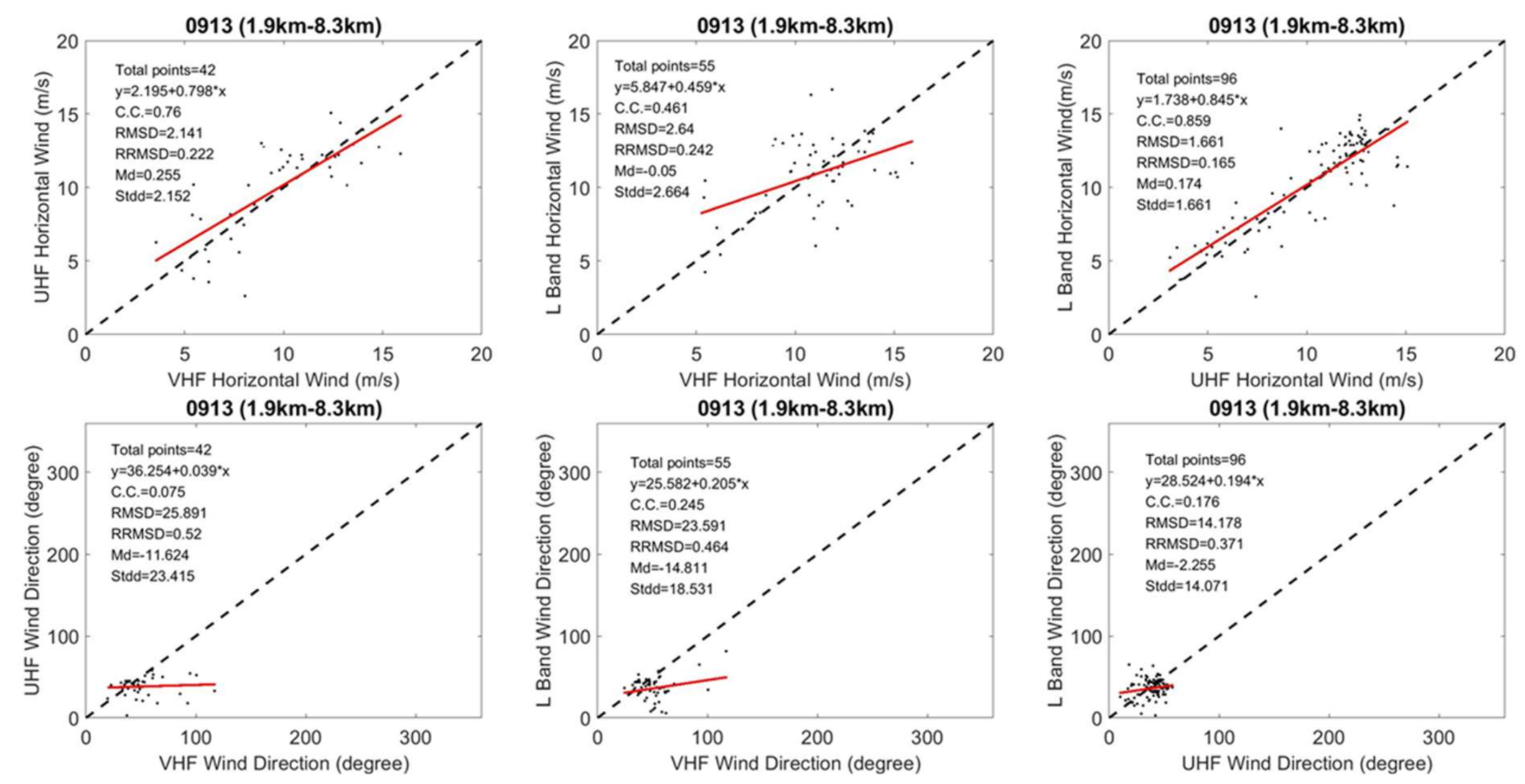
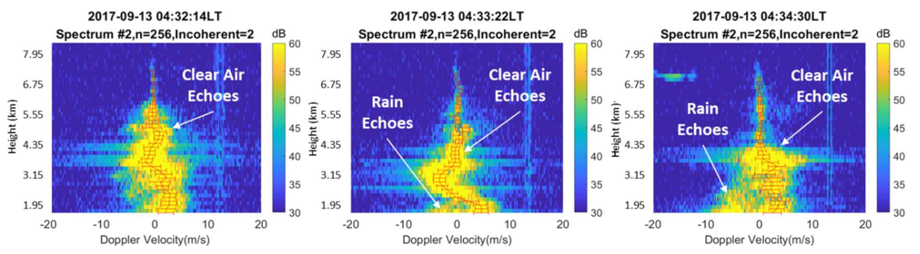
3.3. Wind Velocity Comparisons in Precipitation Conditions

Figure 10 displays the rainfall rates recorded by a 2D video disdrometer manufactured by Joanneum Research for the period of 13–14 September 2017; the device was co-located at the Chung-Li VHF radar site for the campaign experiment. As shown, typhoon-associated heavy precipitation occurred intermittently over the radar site, with a peak rainfall rate of approximately 70 mm hr⁻¹ on 13 September 2017 at around 4 a.m. Figure 11 presents two examples of range variations in the Doppler spectra observed by the eastward (right panel) and westward (left panel) pointed radar beams of the 52 MHz VHF radar in a precipitation environment, in which the positive (negative) Doppler velocity signifies targets moving away from (toward) the radar. As can be seen, the Doppler spectra are very complicated and irregular, in which the clear air turbulence echoes, raindrop echoes, and mixed echoes that were observed both by the main lobe and sidelobe can be clearly discerned. Note that the mixed echoes are the compositions of the radar returns from raindrops, water droplets, and intense turbulence and are characterized by very broad spectral width and intense backscatter in the spectral domain; thus, they are very different from those of the clear air echoes. Therefore, in order to obtain true wind velocities from the radar returns in the precipitation environment, the clear air echoes detected by the main lobe of the radar beam were unambiguously identified and separated from the unwanted echoes. In this study, we used manual inspection to identify and separate the clear air echoes in the Doppler spectral domain for wind velocity estimation in the precipitation environment.

The RMSDs of the wind velocities and directions between different pairs of wind profilers in the presence of precipitation are much larger than those in the absence of precipitation. Figure 12 displays scatterplots of zonal (upper) and meridional (lower) wind velocities between the 52 MHz VHF radar, 449 MHz wind profiler, and 1290 MHz wind profiler in the presence of precipitation. A comparison of Figure 4 and Figure 12 clearly shows that the correlation coefficients of the u and v components between different radar pairs in the presence of precipitation, which are in the range of 0.04–0.74 for the u component and 0.43–0.65 for the v component, are slightly lower than those obtained in the absence of precipitation. In addition, the magnitudes of the RMSDs and Stdds of the former are approximately 2–3 factors larger than the latter on average. As for the MDs, the ratios of the former to the latter are in the range of 4–10. Figure 13 presents the scatterplots of horizontal wind velocity D (upper panels) and wind direction U (lower panels) between three radar pairs in the presence of precipitation. As seen in Figure 13, irrespective of the high correlations of the u and v components shown in Figure 12, the correlations of the U and D between different radar pairs are significantly low, only 0.46–0.86 for U and 0.08–0.25 for D. Nevertheless, the RMSDs and Stdds of U are essentially comparable to those of the u and v components. However, as for the wind direction D, due to the very low correlation coefficients of D, appreciably large RMSD, MD, and Stdd in D can be seen. These features suggest that the wind direction measurements made with wind profilers using the VAD method in the presence of precipitation are rough and unreliable. The values of C.C., RMSD, MD, and Stdd of the horizontal wind velocities and wind directions between radars are summarized in

Table 6. Comparisons of zonal wind (u) and meridional wind velocity (v) between wind profilers in the presence of precipitation.

Radar	VHF-UHF	VHF-L Band	UHF-L Band
Data point	42	55	96
Parameter	u/v	u/v	u/v
C.C.	0.576/0.626	0.039/0.427	0.738/0.648
RMSD (m/s)	2.434/2.890	3.704/3.486	1.909/2.231
MD (m/s)	0.660/−1.338	2.137/−1.878	0.396/−0.492
Stdd (m/s)	2.371/2.592	3.053/2.964	1.877/2.188

and

Table 7. Comparisons of horizontal wind velocity (U) and wind direction (D) between wind profilers in the presence of precipitation.

Radar	VHF-UHF	VHF-L Band	UHF-L Band
Data point	42	55	96
Parameter	U/D	U/D	U/D
C.C.	0.760/0.075	0.461/0.245	0.859/0.176
RMSD (m/s, °)	2.141/25.891	2.640/23.591	1.661/14.179
MD (m/s, °)	0.255/−11.624	−0.050/−14.811	0.174/−2.255
Stdd (m/s, °)	2.152/23.415	2.664/18.531	1.661/14.071

to facilitate comparison.

3.4. Comparison of Vertical Winds

Figure 14 shows three consecutive Doppler spectra with a time resolution of 68 s observed by a vertically pointed radar beam of the 52 MHz VHF radar in a convective precipitation environment, in which the spectral components of clear air and precipitation echoes are clearly identified and marked. From the mean Doppler velocity of the clear air echoes, the vertical wind velocity can thus be acquired. As shown, in the presence of precipitation, the vertical wind velocity at a height of around 3 km varied very dramatically, changing from 2.2 ms⁻¹ upward to −3.2 ms⁻¹ downward within around one minute. This intense downward air motion is very likely the result of the drag effect of the falling raindrops, with a mean terminal velocity of approximately 7 ms⁻¹ in clear air, which were present in a local convective cell moving across the radar beam. In fact, a downdraft with a velocity of approximately −2 ms⁻¹ can also be found at a height of around 3.6 km, and weak echoes from raindrops with terminal velocities of 6–7 ms⁻¹ were present in the height range of 2.3–3.3 km at 04:32:14 LT, which was only one minute before the occurrence of the intense downdraft at around 3 km at 04:33:22 LT. However, the fluctuations in the vertical air velocities in the absence of precipitation were relatively small and mild. Figure 15 displays the vertical wind velocities with a time resolution of 5 min estimated by the VAD method (upper panels) and those observed by the vertically pointed beam (bottom panels) of the 52 MHz Chung-Li VHF radar for clear air (left panels) and precipitation (right panels) environments. As shown, regardless of the methods employed to estimate the vertical wind velocities, they were much more disturbed in the precipitation environment than those in the environment without precipitation. It is obvious from Figure 15 that the height–time distributions of the vertical wind velocities measured by the VAD method were very consistent with those observed by the vertical beam. Nevertheless, there exists a difference in the two. Figure 16 presents histograms of the differences in the vertical wind velocities between the VAD method and vertically pointed radar beam of the 52 MHz Chung-Li VHF radar in clear air conditions (let panel) and the precipitation environment (right panel). As indicated, the mean values of the vertical wind velocity differences between the VAD method and vertical beam measurement are both very small and close to 0. However, the standard deviation of the vertical wind velocity difference in the precipitation environment is around 4.6-times larger than that in the clear air conditions without precipitation. Larsen et al. [40] compared the vertical wind velocities with a time resolution of 65 min between a vertical beam and the VAD method and found that the standard error was approximately 5.3 cms⁻¹, which is much lower than our results (15.3 cms⁻¹ for clear air conditions and 69.4 cms⁻¹ for precipitation environment) with vertical wind data with a 5 min time resolution.

4. Conclusions

In this study, intercomparisons of the horizontal wind velocities measured by multi-frequency radars operating at 52 MHz, 449 MHz, and 1290 MHz on 5 days for the period of 12–16 September 2017 under different atmospheric conditions are made; the devices were co-located on the campus of the National Central University in Taiwan. The results show that correlations of the U, D, u, and v components between different radars are very high, with correlation coefficients in the range of 0.94–0.99 for clear air conditions and 0.04–0.86 for precipitation conditions. The root mean square deviations and standard deviations of the differences between radar-measured wind velocities are very consistent with each other. In the absence of precipitation, the RMSDs of u, v, and U are all in the range of 0.913–1.242 ms⁻¹, with respective mean RMSDs of 0.978, 1.183, and 0.967 ms⁻¹. The range of the RMSDs of the wind direction is 7.7–8.34°, with a mean of 7.944°. In addition, the mean differences (MDs) in u, v, U, and D between different radars are very small and no systematic biases in the radar-measured u, v, U, and D are observed. These results strongly suggest that the horizontal winds measured by the VHF radar, UHF wind profiler, and L-band wind profiler are very accurate, precise, and reliable, despite the operating frequencies of these radars being very different. However, in the presence of precipitation, the RMSDs of the horizontal wind velocities (i.e., u, v, and U) and directions are, respectively, 1.66–3.70 ms⁻¹ and 14.18–25.89°, much larger than those in the absence of precipitation. As for the MDs in the presence of precipitation, they range from −0.05 to 0.26 ms⁻¹ for the horizontal wind velocities and from −14.81° to −2.26° for the directions. Overall, the RMSDs and MDs of the horizontal wind velocities and directions in the presence of precipitation are both substantially larger than those in the absence of precipitation, by a factor of 2–3 for the RMSDs and 3–10 for the MDs. It should be noted that, due to the limited timeframe of the campaign experiment, the data points that we could collect for the comparisons of the horizontal wind velocities between wind profilers and rawinsonde in the presence of precipitation were very limited, which may have affected the precision and accuracy of the statistical results shown in Figure 8 and Figure 9. Therefore, in order to reduce uncertainty and inaccuracy in wind velocity comparison, more data are required for future analysis.

In addition to the intercomparisons of the wind velocities and directions between radars, the radar-measured and rawinsonde-observed winds at the Banqiao meteorological station, located at approximately 26 km northeast of the radar site, are also compared. The results show that the correlations of horizontal wind velocities and directions are still very high, in respective ranges of 0.85–0.96 and 0.94–0.98. In addition, their mean values of RMSDs, MDs, and Stdds of u, v, U, and D are, respectively, 2.808, −1.873, 2.096 ms⁻¹ for u, 2.6, 1.106, 2.389 ms⁻¹ for v, 3.021, −2.064, 2.13 ms⁻¹ for U, and 13.215°, 2.906°, 12.88° for D. An examination indicates that the mean RMSDs and Stdds of the horizontal wind velocities u, v, and U between radar and rawinsonde are around 2–3 factors larger than those between radars. However, the mean MDs of u, v, U, and D between radar and rawinsonde are roughly one order of magnitude larger than those between radars. Therefore, it may be concluded that, in light of the large uncertainty and low accuracy in horizontal wind measurement, the rawinsonde-measured wind velocity should be considered to be inappropriate to serve as a standard reference to assess and evaluate the performance of a wind profiler in atmospheric wind measurement.

References

1. Woodman, R.F.; Guillen, A. Radar observations of winds and turbulence in the stratosphere and mesosphere. J. Atmos. Phys. 1974, 31, 493–505. [Google Scholar] [CrossRef] [Green Version]
2. Green, J.L.; Warnock, J.M.; Winkler, R.H.; van Zandt, T.E. Studies of winds in the upper troposphere with a sensitive VHF ra-dar. Geophys. Res. Lett. 1975, 2, 19–21. [Google Scholar] [CrossRef]
3. Miller, K.L.; Bowhill, S.A.; Gibbs, K.P.; Countryman, I.D. First measurements of mesospheric vertical velocities by VHF radar at temperate latitudes. Geophys. Res. Lett. 1978, 5, 939–942. [Google Scholar] [CrossRef]
4. Czechowsky, P.; Klostermeyer, J.; Röttger, J.; Ruster, R.; Schmidt, G.; Woodman, R.F. The SOUSY-VHF radar for tropo-strato-and mesospheric soundin. In Proceedings of the 17th Conference on Radar Meteorology, Boston, MA, USA, 29 October 2010; American Meteorological Society: Boston, MA, USA; Volume 197, pp. 349–3536. [Google Scholar]
5. Fukao, S.; Sato, T.; Tsuda, T.; Kato, S.; Wakasugi, K.; Makahira, T. The MU radar with an active phased array system: 1. Antenna and power amplifiers. Radio Sci. 1985, 20, 1155–1168. [Google Scholar] [CrossRef]
6. Fukao, S.; Wakasugi, K.; Sato, T.; Morimoto, S.; Tsuda, T.; Hirota, I.; Kimura, I.; Kato, S. The MU radar with an active phased array system: 2. In-house equipment. Radio Sci. 1985, 20, 1169–1176. [Google Scholar] [CrossRef]
7. Chao, J.K.; Kuo, F.S.; Chu, Y.S.; Fu, I.J.; Röttger, J.; Liu, C.H. The first operation and results of the Chung-Li VHF radar. In Handbook for MAP; Bowhill, S.A., Edwards, B., Eds.; SCOSTEP Secr., University of Illinois: Urbana, IL, USA, 1986; Volume 20, pp. 359–363. [Google Scholar]
8. Röttger, J.; Liu, C.H.; Chao, J.K.; Chen, A.J.; Chu, Y.H.; Fu, I.J.; Huang, C.M.; Kiang, Y.W.; Kuo, F.S.; Lin, C.H.; et al. The Chung-Li VHF radar: Technical layout and a summary of initial results. Radio Sci. 1990, 25, 487–502. [Google Scholar] [CrossRef]
9. Briggs, B.H.; Candy, B.; Elford, W.G.; Hocking, W.K.; May, P.T.; Vincent, R.A. The Adelaide VHF radar-capabilities and future plans. Handb. MAP 1984, 14, 357–359. [Google Scholar]
10. Bertin, F.; Cremieu, A.; Glass, M.; Massebeuf, M.; Ney, R.; Petitdidier, M. The PROUST radar: First results. Radio Sci. 1987, 22, 51–60. [Google Scholar] [CrossRef]
11. Crochet, M. Characteristics of Provence radar. Handb. MAP 1989, 28, 491–492. [Google Scholar]
12. Rao, P.B.; Jain, A.R.; Kishore, P.; Balamuralidhar, P.; Damle, S.H.; Viswanathan, G. Indian MST radar: 1. System description and sample wind measurements in ST mode. Radio Sci. 1995, 30, 1125–1138. [Google Scholar] [CrossRef]
13. Slater, K.; Stevens, A.D.; Pearmain SA, M.; Eccles, D.; Hall, A.J.; Bennett RG, T.; France, L.; Roberts, G.; Olewicz, Z.K.; Thomas, L. Overview of the MST radar system at Aberystwyth. In Proceedings of the Fifth Workshop on Technical and Scientific Aspects of MST Radar, Aberystwyth, UK, August 6–9 1991; pp. 479–482. [Google Scholar]
14. Anonymous. Technological and Scientific Opportunities for Improved Weather and Hydrological Services in the Coming Decade. Report to the National Weather Service by the Select Committee on the National Weather Service, Assembly of Mathematical and Physical Sciences; National Research Council: Washington, DC, USA, 1980; p. 87. [Google Scholar]
15. Balsley, B.B.; Gage, K.S. On the Use of Radars for Operational Wind Profiling. Bull. Am. Meteorol. Soc. 1982, 63, 1009–1018. [Google Scholar] [CrossRef] [Green Version]
16. van Zandt, T.E. A brief history of the development of wind-profiling or MST radars. Ann. Geophys. 2000, 18, 740–749. [Google Scholar] [CrossRef]
17. Woodman, R.F.; Chu, Y.H. Aspect sensitivity measurements of VHF backscatter made with the Chung-Li radar: Plausible mechanism. Radio Sci. 1989, 24, 113–125. [Google Scholar]
18. Weber, B.L.; Wuertz, D.B. Comparison of rawinsonde and wind profiler radar measurements. J. Atmos. Ocean. Technol. 1990, 7, 157–174. [Google Scholar] [CrossRef] [Green Version]
19. May, P.T. Comparison of wind-profiler and radiosonde measurements in the tropics. J. Atmos. Ocean. Technol. 1993, 10, 112–127. [Google Scholar] [CrossRef]
20. Saïd, F.; Campistron, B.; Delbarre, H.; Canut, G.; Doerenbecher, A.; Durand, P.; Fourriè, N.; Lambert, D.; Legain, D. Offshore winds obtained from a network of wind-profiler radars during HyMeX. Q. J. R. Meteorol. Soc. 2016, 142 (Suppl. 1), 23–42. [Google Scholar] [CrossRef]
21. Kottayil, A.; Mohanakumar, K.; Samson, T.; Rebello, R.; Manoj, M.G.; Varadarajan, R.; Santosh, K.R.; Mohanan, P.; Vasudevan, K. Validation of 205 MHz wind profiler radar located at Cochin, India, using radiosonde wind measurements. Radio Sci. 2016, 51, 106–117. [Google Scholar] [CrossRef] [Green Version]
22. Kim, M.-S.; Bernard, C.; Byung, H.K. Frontal Wind Field Retrieval Based on UHF Wind Profiler Radars and S-Band Radars Network. Atmosphere 2019, 10, 547. [Google Scholar] [CrossRef] [Green Version]
23. Mohanakumar, K.; Kottayil, A.; Aanadan, V.K.; Samson, T.; Thomas, L.; Satheesan, K.; Rebello, R.; Manoj, M.G.; Varadarajan, R.; Santosh, K.R.; et al. Technical Details of a Novel Wind Profiler Radar at 205MHz. J. Atmos. Ocean. Technol. 2017, 34, 2659–2671. [Google Scholar] [CrossRef]
24. Browning, K.A.; Wexler, R. The determination of kinematic properties of a wind field using Doppler radar. J. Appl. Meteorol. 1968, 7, 105–113. [Google Scholar] [CrossRef]
25. Wilson, D.A. The Kinematic Behavior of Spherical Particles in an Accelerating Environment; NOAA Tech. Rep. ERL 187-WPL 13; U.S. Government Printing Office: Boulder, CO, USA, 1970.
26. Ishii, S.; Mizutani, K.; Aoki, T.; Sasano, M.; Murayama, Y.; Itabe, T.; Asai, K. Wind Profiling with an Eye-Safe Coherent Doppler Lidar System: Comparison with Radiosondes and VHF Radar. J. Meteorol. Soc. Jpn. 2005, 83, 1041–1056. [Google Scholar] [CrossRef] [Green Version]
27. Strauch, R.G.; Webb, B.L.; Frisch, A.S.; Little, C.G.; Merritt, D.A.; Moran, K.P.; Welsh, D.C. The precision and relative accuracy of profiler wind measurements. J. Atmos. Ocean. Technol. 1987, 4, 563–571. [Google Scholar] [CrossRef] [Green Version]
28. Larsen, M.F. Can a VHF Doppler Radar Provide Synoptic Wind Data? A Comparison of 30 Days of Radar and Radiosonde Data. Mon. Weather Rev. 1983, 111, 2047–2057. [Google Scholar] [CrossRef] [Green Version]
29. Strauch, R.G.; Merritt, D.A.; Moran, K.P.; Earnshaw, K.B.; van de Kamp, D. The Colorado Wind profiling Network. J. Atmos. Ocean. Technol. 1984, 1, 37–49. [Google Scholar] [CrossRef] [Green Version]
30. Rao, I.S.; Anandan, V.K.; Reddy, P.N. Evaluation of DBS Wind Measurement Technique in Different Beam Configurations for a VHF Wind Profiler. J. Atmos. Ocean. Technol. 2008, 25, 2304–2312. [Google Scholar] [CrossRef]
31. Fukao, S.; Sato, T.; Yamasaki, N.; Harper, R.; Kato, S. Winds Measured by a UHF Doppler Radar and Rawinsondes—Comparisons Made on Twenty-Six Days (August–September 1977) at Arecibo, Puerto Rico. J. Appl. Meteorol. 1982, 21, 1357–1363. [Google Scholar] [CrossRef]
32. Chu, Y.H.; Chao, J.K.; Liu, C.H.; Rottger, J. Aspect sensitivity at tropospheric heights measured with vertically pointed antenna beam of the Chung-Li VHF radar. Radio Sci. 1990, 25, 539–550. [Google Scholar] [CrossRef]
33. Chu, Y.H.; Wang, C.Y. Interferometry observations of 3-dimensional spatial structures of sporadic E irregularities using Chung-Li VHF radar. Radio Sci. 1997, 32, 817–832. [Google Scholar] [CrossRef]
34. Su, C.L.; Chen, H.C.; Chu, Y.H.; Chung, M.Z.; Kuong, R.M.; Lin, T.H.; Tzeng, K.J.; Wang, C.Y.; Wu, K.H.; Yang, K.F. Meteor radar wind over Chung-Li (24.9°N, 121°E), Taiwan, for the period 10–25 November 2012 which includes Leonid meteor shower: Comparison with empirical model and satellite measurements. Radio Sci. 2014, 49, 597–615. [Google Scholar] [CrossRef] [Green Version]
35. Chen, J.S.; Chu, Y.H. A discussion on the variations of MST/ST radar echo power with a turbulent layer resolved by the frequency domain interferometry technique. Radio Sci. 2000, 35, 1375–1387. [Google Scholar] [CrossRef] [Green Version]
36. Chen, C.-H.; Su, C.-L.; Chen, J.-H.; Chu, Y.-H. Vertical Wind Effect on Slope and Shape Parameters of Gamma Drop Size Distribution. J. Atmos. Ocean. Technol. 2020, 37, 2243–2262. [Google Scholar] [CrossRef]
37. Lee, C.F.; Vaughan, G.; Hooper, D.A. Evaluation of wind profiles from the NERC MST radar, Aberystwyth, UK. Atmos. Meas. Tech. 2014, 7, 3113–3126. [Google Scholar] [CrossRef] [Green Version]
38. Päschke, E.; Leinweber, R.; Lehmann, V. An assessment of the performance of a 1.5μm Doppler lidar for operational vertical wind profiling based on a 1-year trial. Atmos. Meas. Tech. 2015, 8, 2251–2266. [Google Scholar] [CrossRef] [Green Version]
39. Haefele, A.; Ruffieux, D. Validation of the 1290 MHz wind profiler at Payerne, Switzerland, using radiosonde GPS wind measurements. Meteorol. Appl. 2015, 22, 873–878. [Google Scholar] [CrossRef] [Green Version]
40. Larsen, M.F.; Fukao, S.; Aruga, O.; Yamanaka, D.; Tsuda, T.; Kato, S. A comparison of VHF radar vertical-velocity measurements by a direct vertical-beam method and by a VAD method. J. Atmos. Ocean. Technol. 1991, 8, 766–776. [Google Scholar] [CrossRef] [Green Version]
Figure 1. Antenna arrays of the wind profiler radars operated at 52 MHz, 449 MHz, and 1290 MHz, deployed at the campus of National Central University (left), and antenna beam pattern of obliquely pointed radar beam for Chung-Li VHF radar (right).
Atmosphere 12 01284 g001
Figure 2. Doppler spectra observed by the north-pointed (left) and south-pointed oblique radar beams of the Chung-Li VHF radar, in which the spctral components of the radar returns received by the main lobe and side lobe are present.
Atmosphere 12 01284 g002
Figure 3. (a) Height–time–intensity plots of zonal wind velocities measured by VHF radar (top panels), UHF radar (middle panels), and L-band radar (bottom panels) on 12 September, 15 September, and 16 September 2017 in clear air conditions without precipitation; (b) Same as Figure 3a, but for meridional wind velocities.
Atmosphere 12 01284 g003
Figure 4. Comparisons of zonal (upper) and meridional (lower) wind velocities measured by 52 MHz VHF radar, 449 MHz wind profiler, and 1290 MHz wind profiler for clear air conditions.
Atmosphere 12 01284 g004
Figure 5. Scatterplots of horizontal wind velocities (upper) and wind directions (lower) between different pairs of wind profiler measurements in clear air conditions. The dashed black line is the diagonal line, and solid red line is the regression line best fit to the data.
Atmosphere 12 01284 g005
Figure 6. Comparisons of the horizontal wind velocities (upper panels) and wind directions (bottom panels) measured by 52 MHz radar (red curve), 449 MHz wind profiler (blue curve), 1290 MHz profiler (green curve), and radiosonde (black curve) in clear air conditions.
Atmosphere 12 01284 g006
Figure 7. Same as Figure 6, but for zonal (upper) and meridional (lower) wind velocities.
Atmosphere 12 01284 g007
Figure 8. Comparison of horizontal wind velocities (upper panels) and wind directions (lower panels) between wind profiler and radiosonde measurements in clear air conditions. The dashed black line is the diagonal line, and the solid red line is the linear fit to the data.
Atmosphere 12 01284 g008
Figure 9. Comparisons of radar-measured horizontal wind velocities and radiosonde wind for zonal (upper) and meridional (lower) wind components in clear air conditions. The dashed black line is the diagonal line, and the solid red line is the linear fit to the data.
Atmosphere 12 01284 g009
Figure 10. Time series of rainfall rate measured by a ground-based disdrometer co-located at the Chung-Li radar station.
Atmosphere 12 01284 g010
Figure 11. Examples of Doppler spectra observed by obliquely pointed radar beam of the 52 MHz VHF radar in precipitation environment, in which spectral components of clear air echoes, raindrop echoes, and mixed echoes, which are the combination of echoes from raindrops, water droplets, and clear air turbulence, are marked.
Atmosphere 12 01284 g011
Figure 12. Comparison of zonal (upper) and meridional (lower) wind velocities between 52 MHz VHF radar, 449 MHz wind profiler, and 1290 MHz wind profiler for precipitation conditions.
Atmosphere 12 01284 g012
Figure 13. Same as Figure 12, but for horizontal wind velocity (upper) and wind direction (lower).
Atmosphere 12 01284 g013
Figure 14. Examples of Doppler spectra observed by vertically pointed radar beam of the 52 MHz VHF radar in precipitation environment, in which spectral components of clear air and precipitation echoes are clearly seen.
Atmosphere 12 01284 g014
Figure 15. Vertical wind velocities estimated by VAD method (upper panels) and observed by vertically pointed beam (bottom panels) of 52 MHz Chung-Li VHF radar for clear air (left panels) and precipitation (right panels) environments.
Atmosphere 12 01284 g015
Figure 16. Histograms of vertical wind differences between VAD method and vertical beam observations in clear air conditions (left) and precipitation environment (right) for the data shown in Figure 15.
Atmosphere 12 01284 g016