Air Flow Experiments on a Train Carriage—Towards Understanding the Risk of Airborne Transmission

Abstract

A series of experiments was undertaken on an intercity train carriage aimed at providing a “proof of concept” for three methods in improving our understanding of airflow behaviour and the accompanied dispersion of exhaled droplets. The methods used included the following: measuring CO₂ concentrations as a proxy for exhaled breath, measuring the concentrations of different size fractions of aerosol particles released from a nebuliser, and visualising the flow patterns at cross-sections of the carriage by using a fog machine and lasers. Each experiment succeeded in providing practical insights into the risk of airborne transmission. For example, it was shown that the carriage is not well mixed over its length, however, it is likely to be well mixed along its height and width. A discussion of the suitability of the fresh air supply rates on UK train carriages is also provided, drawing on the CO₂ concentrations measured during these experiments.

1. Introduction

The COVID-19 pandemic has resulted in a much decreased capacity on UK rail services, with physical distancing rules applied for much of the pandemic that force trains to operate at half capacity or less. According to Department for Transport (DfT) statistics, following the first UK lockdown, passenger numbers have remained well below capacity [1]. This is likely due to the large increase in the number of people working from home resulting in a reduction in passenger numbers during peak hours and people’s tendency to avoid non-essential travel due to concerns regarding the risk of infection by the SARS-CoV-2 virus while travelling. Travel by public transport such as rail is perceived by some commentators as potentially high risk due to the potential of interacting with a large number of people at the station, the possibility of being in close proximity to other people during the journey, and the requirement of spending extended periods of time within a confined space with others.

These concerns may not be entirely unfounded and any train journey inevitably carries a degree of risk of infection by the SARS-CoV-2 virus, particularly as exposure to asymptomatic individuals is seen as a major mode of transmission [2]. Infection can occur via three routes: by contact with infected surfaces, droplet transmission, and airborne transmission [3,4,5,6]. Transmission via surface contact is mitigated by regular cleaning of touch points, the use of antimicrobial products that can provide a degree of residual protection, provision of hand sanitiser in stations, and promotion of regular hand washing. By “droplet transmission”, we refer to transmission via large droplets exhaled while coughing or sneezing and also, to a lesser degree, while breathing or talking. Larger droplets fall to the ground within seconds [7,8]; therefore, enforcing physical distancing and, with sufficient levels of compliance, wearing masks are effective mitigation strategies against this transmission route. By “airborne transmission”, we refer to the transmission of the virus via smaller particles that tend to follow the dominant airflow patterns within a space and can remain in the air for extended periods of time (minutes to hours). There exists considerable evidence to suggest that airborne transmission of SARS-CoV-2 is viable [9]; therefore, appropriate mitigation measures should be taken against this transmission route [3,4,5,6,10]. However, mitigation strategies continue to be mainly focused on surface contact and droplet transmission only.

The risk of airborne transmission is likely to be higher in small spaces such as a train carriages, especially if ventilation rates are low. In these cases, virus-laden particles exhaled by an infected person can accumulate and result in high doses for uninfected persons within the space. In addition to the provision of fresh outdoor air, the risk of airborne transmission is likely to depend on the airflow patterns within the space. For example, areas within a space with low airflow velocities could result in an accumulation of infected air with virus-laden aerosols. Thermal stratification within a space can restrict vertical mixing of air and result in high concentrations of virus-laden particles in certain zones, potentially including the breathing zone. Therefore, when assessing the relative risk of airborne transmission indoors, it is important to have an understanding of both the outdoor air supply and the airflow patterns within the space. Alternatively, CO${}_2$ concentrations can be measured to provide an estimate of the concentrations of exhaled breath within the space, and the risk of transmission can be estimated in turn [11,12,13].

Public transport poses a unique challenge when evaluating the risk of airborne transmission and when seeking to establish suitable mitigation strategies. Firstly, the ventilation rates for vehicles with some degree of natural ventilation (i.e., windows that can be opened) can vary significantly depending on the speed of travel and the number of open windows. The exchange of air when doors are opened to allow passengers to board and alight should also be considered and also applies to vehicles that are otherwise entirely mechanically ventilated. Estimating the ventilation rate on buses or trains is, therefore, often difficult. The problem is compounded by the wide range of carriage types in operation, which all have different dimensions and ventilation configurations. Secondly, plumes driven by body heat can have a significant impact on the airflow patterns within vehicles [14,15,16,17,18], which in turn can vary depending on the number and location of occupants. Of course, the distribution of the airborne pathogen within the vehicle can depend on the location of the infectious individual. The heating of surfaces by solar radiation can also affect airflow within the vehicle on sunny days [14,15,19]. Furthermore, the movement of people has been shown to have a considerable impact on the mixing of airborne contaminants indoors [20] and is likely to play a significant role in vehicles, particularly during busy periods. Finally, buses and trains are long and narrow with few access points. Therefore, it is often difficult to avoid being in close proximity with other passengers. Furthermore, the long, narrow shape is likely to cause the airflow patterns within the space to be particularly sensitive to the location of the air inlet and extract vents.

An understanding of the outdoor air provision in addition to the airflow patterns within public transport vehicles is, therefore, essential in order to effectively mitigate the risk of airborne transmission. The literature on airflow patterns within buses and trains is focused mainly on assessing the thermal comfort of passengers, e.g., [14,15,16,17,18,19]. In [21,22], respiratory droplet transmission within a train carriage is modelled using Reynolds-Averaged Navier–Stokes (RANS) computational fluid dynamics (CFD). These consider different ventilation configurations for carriages of high-speed trains in China. The range of dispersion of droplets, in addition to their residence time within the carriage, is shown to vary significantly for the different ventilation outlet positions considered. CFD studies of airborne transmission on a bus include [23,24], who demonstrated the sensitivity of the likelihood of transmission on a bus to the location of the infected person relative to the extract vent. Considerable effort has been made in understanding and modelling the airborne transmission of pathogens within aircraft cabins, e.g., [25,26,27,28]. Mazumdar and Chen [27] used a one-dimensional diffusion model to predict the concentrations of a gaseous contaminant along the length of an airliner cabin, while [29,30] used a zonal model. In [31], aerosol droplets were released within the cabin of aircraft, and concentrations were measured at various locations. It was shown that the very high air recirculation rates within commercial aircraft are very effective in diluting aerosol particle concentrations. In [32,33,34], it was shown that acceleration-induced body forces occurring during both the climb and descent stages of flight can affect the dispersion of a contaminant and the resulting exposure of passengers.

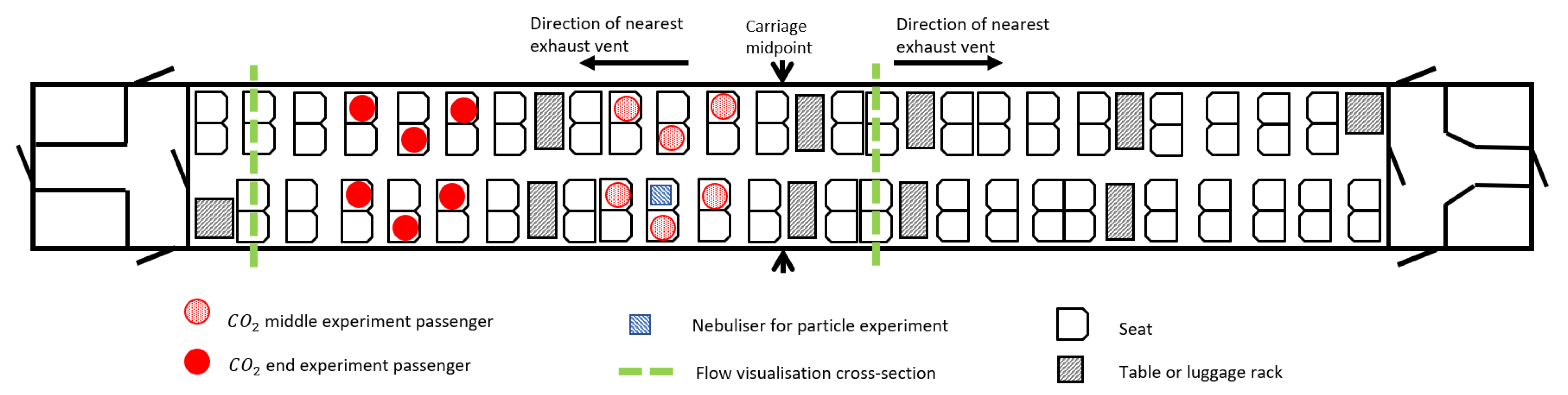
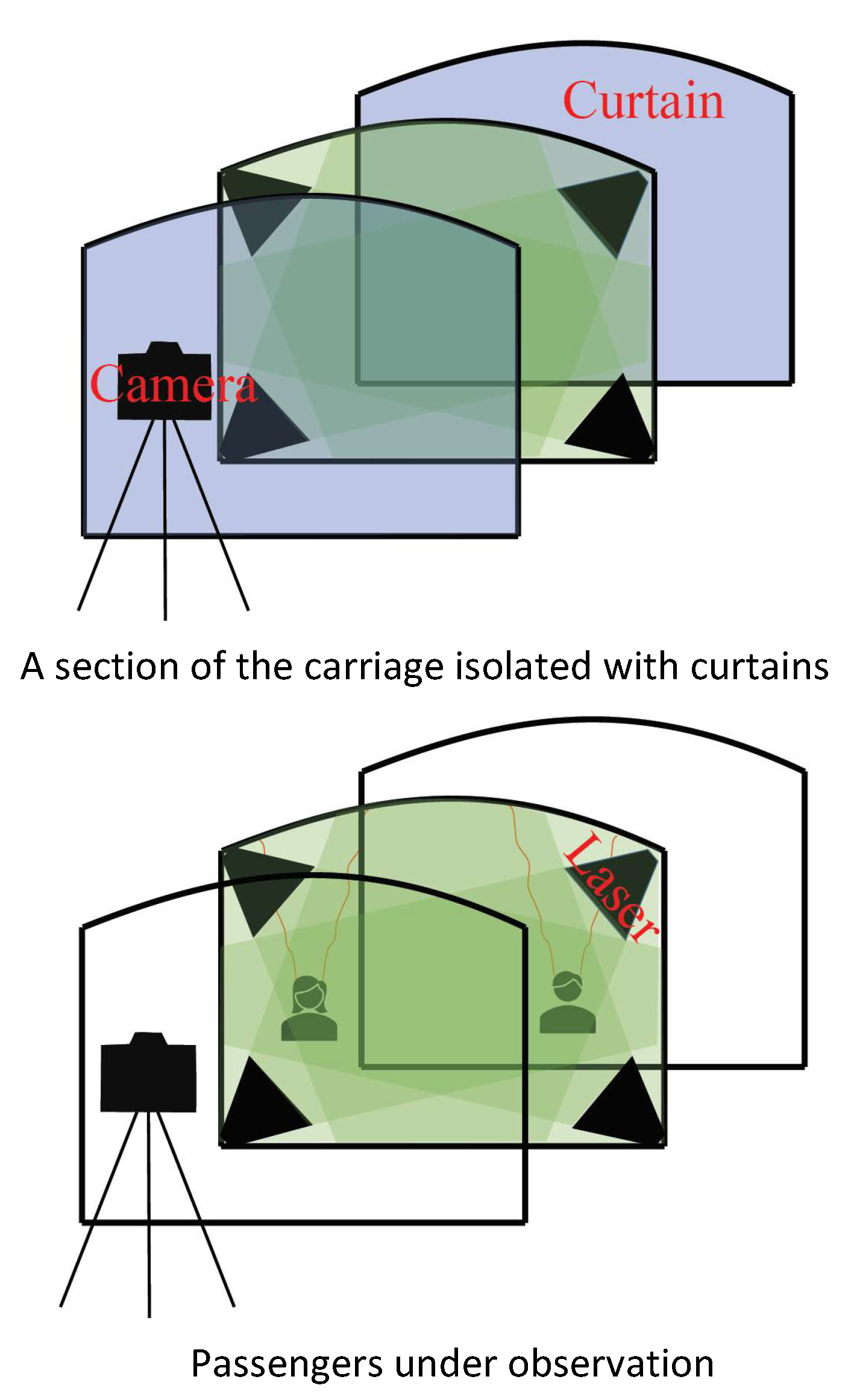
While examples of CFD studies of airflow behaviour in vehicles can be found in the literature, there are few examples of full-scale experiments in public transport vehicles. In this paper, we outline the experimental procedure for three experiments implemented on an inter-city train carriage in the UK. These experiments included measuring CO${}_2$ generated by volunteer “passengers”, flow visualisations of artificial smoke released within the carriage, and the measurement of the concentrations of aerosols released from a nebuliser. The aim in each case was to improve our understanding of the airflow patterns and aerosol dispersion within the carriage and to determine the utility of each method. Time for planning and executing these experiments was limited; therefore, some of the experimental standards normally expected were not met. For example, we could not perform the desired number of repeat runs. However, sufficient data were gathered to provide a demonstration of “proof of concept”, while also providing insights into the airflow behaviour within the carriage.

2. Materials and Methods

2.1. Carriage Layout and Ventilation

The carriage used for the experiments consists of a passenger saloon and two vestibules at either end. This carriage layout is similar to other types of intercity carriages running on the GB rail network, but it is different from a typical carriage on a commuter/regional network, which are more common and more heavily used. The saloon takes the majority of the space inside the carriage (Figure 1) and includes 88 seats. The volume of the saloon is approximately 113 m${}^3$, while the volume of the entire carriage is approximately 140 m${}^3$. The majority of seats are in an “airline” configuration, however, some seats face each other across a table. There is a door at both ends of the saloon, which leads to a vestibule. These internal doors open automatically when approached but are otherwise shut. Each vestibule has a door on either side for passenger boarding and alighting, along with a third door for access to the next carriage.

The carriage is mechanically ventilated, and the windows within the carriage cannot be opened. Two Heating, Ventilation, and Air Conditioning (HVAC) units are located on the roof, one at each end of the carriage. These units provide a supply of outdoor air to the saloon and vestibules, drive the flow of conditioned air within the carriage, and can either heat or cool the air as required. The conditioned air, which is a mixture of outdoor air and recirculated air, is vented into the saloon from the ceiling along the entire length of the carriage (Figure 2). The extract vent for each ventilation unit is located on the ceiling at each end of the saloon. Heaters are located near the floor along each wall of the saloon to provide additional heating capacity to supplement that the ventilation system.

The carriage ventilation system can be set to operate in several different modes: automatic heating or cooling and forced cooling or forced heating. The outdoor temperature was above 30 ${}^{\circ }$C during the days of these experiments; therefore, forced cooling was chosen as the ventilation setting used for each experiment. Forced cooling can be run at several different cooling rates, from 0% to 100%. A 75% cooling capacity was used, and the desired temperature within the saloon was set to 21 ${}^{\circ }$C at the HVAC control unit. The exact flow rates of outdoor air provided to the carriage and the flow rates of recirculated air were not known. However, the design specification of the carriage HVAC system specified a fresh air supply in the range of 22.5–30 m${}^3$ min${}^{-1}$ and a recirculation flow rate of 30–60 m${}^3$ min${}^{-1}$. The heaters remained switched off at all times.

2.2. Outline of Experiments

2.2.1. CO${}_2$ Experiment

The objective of the CO${}_2$ experiments was to explore the feasibility of using CO${}_2$ generated by exhaled breath and CO${}_2$ sensors to resolve concentration differences within the saloon and to observe whether ventilation removed any stratification.

The CO${}_2$ experiments involved the generation of CO${}_2$ by members of the research team representing passengers and sitting in the carriage while the ventilation was switched off, allowing CO${}_2$ concentrations to rise before switching the ventilation on and measuring the decay rate of CO${}_2$ at several locations. Six members of the research team acted as passengers and sat in the carriage for a total of 35 min at a time. The passengers were arranged to maximise the distance between each passenger while occupying three rows of seats. This resulted in a staggered formation as shown in Figure 3 and Figure 4, as well as Figure 1. The ventilation was switched off at the start of the experiment. After 15 min, the ventilation was switched on and used the 75% forced cooling setting. The passengers remained in their seats for an additional 20 min before the experiment was stopped. The experiments were carried out at two locations within the saloon: the first near the midpoint of the saloon and the second near the end of the saloon. Both experiments were run twice.

Seven CO${}_2$ sensors (K33-LP T, SenseAir AB, Delsbo, Sweden) were placed at various locations within the carriage (Figure 3 and Figure 4). The sensors were calibrated with a reference analyser (G2201-i, Picarro Inc., Santa Clara, USA). The percentage error of reading was within 3% in the range of 0–3000 ppm. These sensors are labelled M1 to M7. Sensors M3 and M5 were placed on the backs of seats at the height of the typical breathing zone for sitting passengers and in close proximity to the six passengers. M6 and M7 were also placed at the back of a seat but at a greater distance from the passengers. M4 was placed on the luggage rack, while M1 was attached to the ceiling. Sensors M1, M4, and M5 were all located at the same distance along the length of the carriage. For the first experiment near the midpoint of the carriage, M2 was placed on the back of a seat on the opposite side to M6, closer to the extract vent. For the experiment at the end of the carriage, M2 was placed on the luggage rack above M7 and directly below the extract vent.

The experiments reported here were performed during the ongoing COVID-19 pandemic. The experimental procedure was, therefore, complicated by the necessity to mitigate the risk of infection from any potentially asymptomatic participating researchers. With this in mind, the time period during which the passengers were asked to sit in close proximity with the ventilation off was limited to 15 min. An additional 20 min was allowed with the ventilation switched on. Due to these relative short time periods, a steady state in CO${}_2$ concentrations was never reached, either during the ventilation off or ventilation on period. Furthermore, due to the limited time available on the carriage, only two runs of each experiment were performed.

2.2.2. Aerosol Dispersion Experiment

The aim of the particle dispersion experiment was to map the aerosol distribution over adjacent seats during a continuous release of aerosols under the ventilation off and on conditions. The size of exhaled droplets ranges between 0.01 and 1000 $\mathsf{\mu }$m [35]; therefore, it is important to consider the dispersion of different aerosol size fractions. A nebuliser was used as a source to generate continuous aerosols made up of sodium chloride solution (salt; 1% by weight) at a flow rate of 6 L per minute, which is within the range of the human breathing rate, typically 5–7 L/min${}^{-1}$ while resting [36]. The use of a nebuliser allowed us to investigate the significance of droplet mass on dispersion. The aerosol particles released by the nebuliser had a size range of 0.25 $\mathsf{\mu }$m to 16.5 $\mathsf{\mu }$m. Six laser particle counters (Dylos1700) were used to measure concentrations of fine (${\mathrm{PM}}_{2.5}$; aerodynamic diameter $\le 2.5\mathsf{\mu }$m) and coarse (${\mathrm{PM}}_{10}$; aerodynamic diameter $\le 10\mathsf{\mu }$m) aerosol particles at different adjacent seats (Figure 5). These aerosol monitors have been successfully deployed in previous work [37,38]. As for the CO${}_2$ experiments, a 75% forced cooling setting was used for the “ventilation on” period of these experiments. There were no passengers present during this experiment; therefore, the effects of body plumes and people movement were not considered.

As part of quality control and assurance process, we carried out co-location measurements over a period of 8 h prior to the experiments in order to assess relative accuracy. Pearson correlation coefficients (r) greater than 0.93 and 0.87 were observed for ${\mathrm{PM}}_{2.5}$ and ${\mathrm{PM}}_{10}$, respectively, as observed in Figure A1.

The aerosol monitors were mounted on the back of seats at the typical breathing height of a sitting passenger (1.2 m above the floor) at various locations near the nebuliser (Figure 5). A total of six sets of experiments, each for 25 min, were conducted under both “ventilation off” (indoor cabin temperature, T = 32.3 ± 1.2 ${}^{\circ }$C; relative humidity, RH = 39.5 ± 2.9%) and on (T = 30.8 ± 0.2 ${}^{\circ }$C; RH = 40.3 ± 2.5%) conditions. Before each experiment, the ventilation was switched on for 15 min to clear the accumulated concentrations over the measurement duration and to reach a stabilised background aerosol concentration level. Another 5 min was allowed before the start of each experiment after switching the ventilation on or off in order to allow the carriage flow to reach a quasi-steady-state condition.

The six aerosol monitors located at different locations within a cabin were marked as $B_{100}$, $B_{70}$, $S_0$, $S_{45}$, $F_{70}$, and $F_{140}$; B, F, and S refer to behind, in front, and the same row as the seat on which the nebuliser was placed, respectively. The nebuliser release faced towards the “front” direction. The subscript indicates the horizontal distance in cm with respect to the source (Figure 5). For example, $F_{70}$ and $B_{70}$ indicate that these aerosol monitors were placed in front of and behind the source seat, respectively, at a distance of 70 cm from the source ($S_0$). $S_{45}$ refers to the seat in the same row as $S_0$ at a distance of 45 cm. The monitor at $S_0$ was placed directly below the nebuliser outlet, within a few centimetres. The nearest ventilation extract was located behind the nebuliser’s seat.

The following equation was used to normalise the measured aerosol concentrations in order to understand the aerosol concentrations in relative terms so that the concentration ranged between 0 and 1.

$$C_{norm}=\frac{\mathrm{Average}\mathrm{aerosol}\mathrm{concentration}\mathrm{at}\mathrm{a}\mathrm{location}}{\mathrm{Average}\mathrm{aerosol}\mathrm{concentration}\mathrm{at}\mathrm{source}}.$$

(1)

The R statistical software (R Core Team, 2019) in the Open-air software package [39] was used to carry out data processing and statistical analyses.

2.2.3. Airflow Visualisation

The dominant flow patterns across the width and height of the carriage were visualised both near the middle and the end of the saloon. The locations of the visualised cross-sections are indicated in Figure 1 by the green dashed lines. Flow pattern visualisation was conducted by tracing the motion of a neutrally buoyant, inert fog under the ventilation flow.

Lasers (30 mW; 520 nm) were fitted with Powell lenses in order to form a diverging laser sheet and then mounted and aligned in order to illuminate the fog across a carriage cross-section. In order to enhance visualisation, the lights in the carriage were switched off, and plastic blackout sheets were used to cover the windows. Initially, the ventilation within the carriage was switched off. A section of the carriage approximately 2 m in length was isolated by using curtains before being filled with non-toxic, artificial, and theatrical smoke consisting of 70% water and 30% glycol droplets of size ranges between 5 and 10 $\mathsf{\mu }$m. Once the carriage section was suitably filled, the plastic sheets were removed, and two passengers sat on either side of the aisle such that the illuminated cross-section of the carriage passed over their shoulders and heads (see Figure 6). Once in position, the flow generated by the body plumes of the passengers was allowed to develop before the ventilation was switched on (75% forced cooling). The flow was visualised until the fog was dispersed to a degree that visualisation was no longer effective. Typically, this allowed a minute or two of visualisation.

3. Results

3.1. CO${}_2$ Experiment

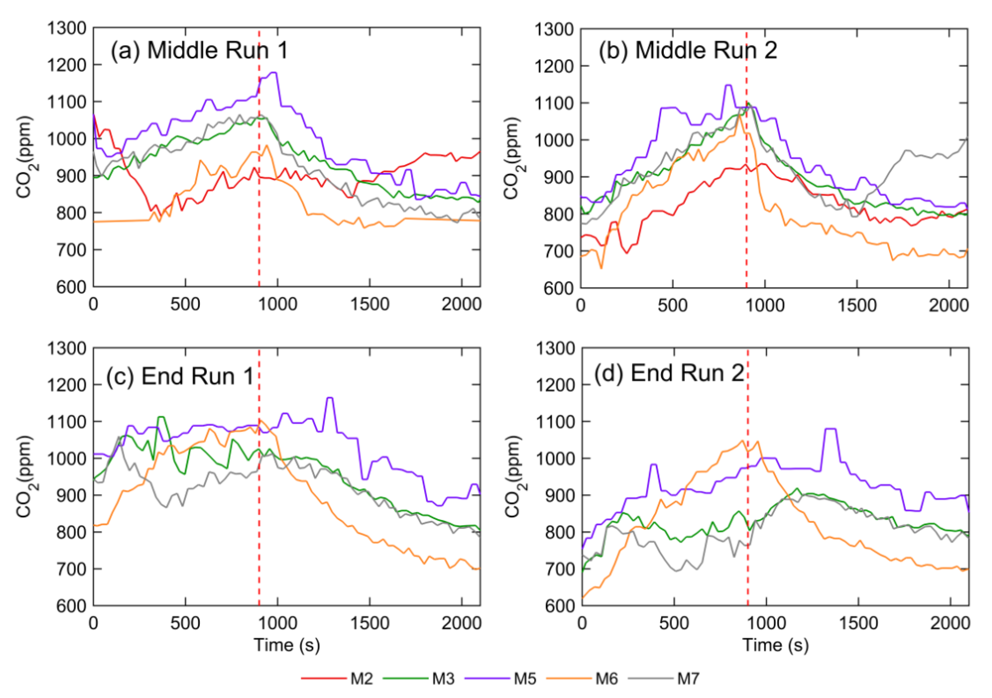
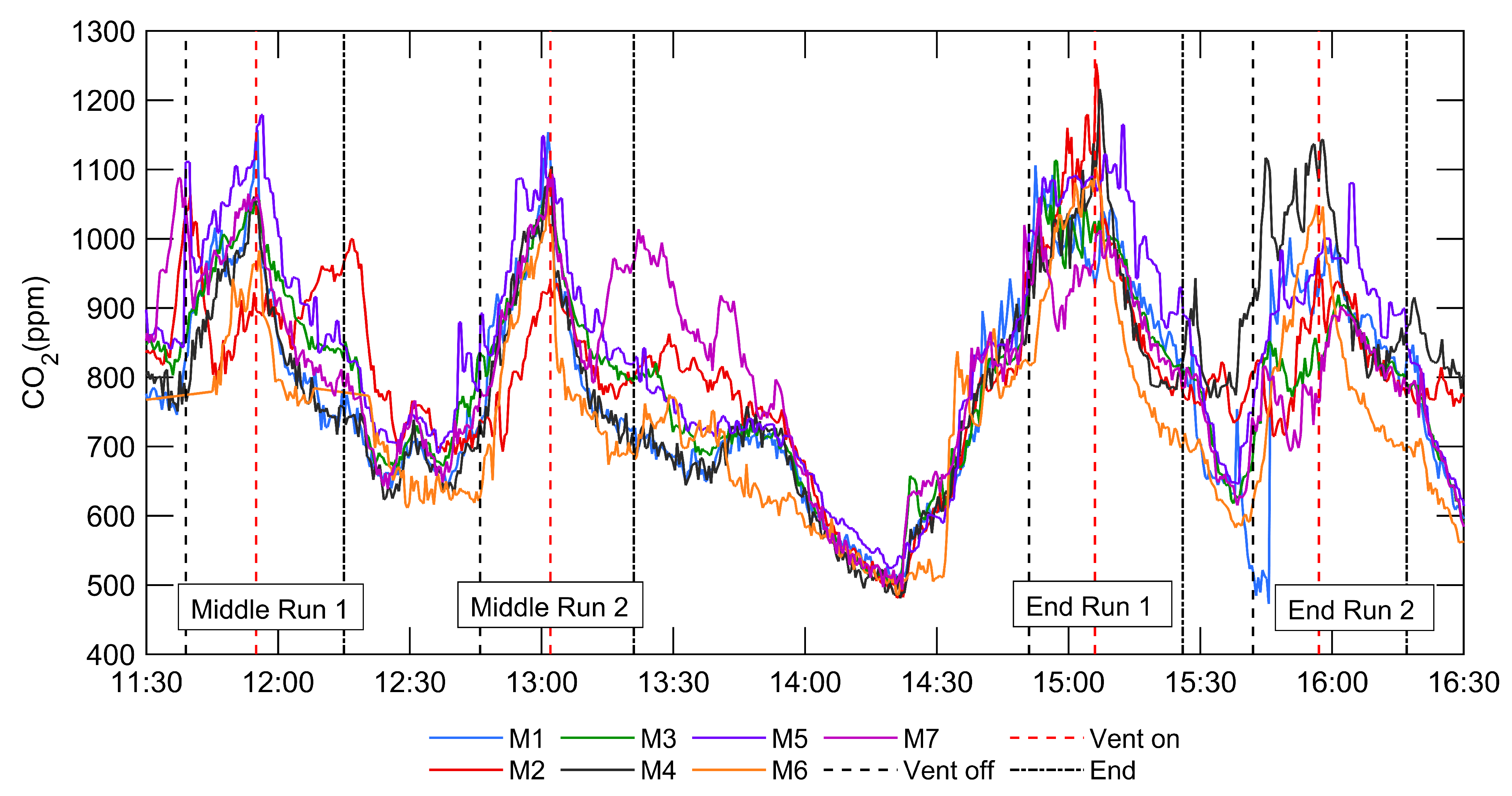
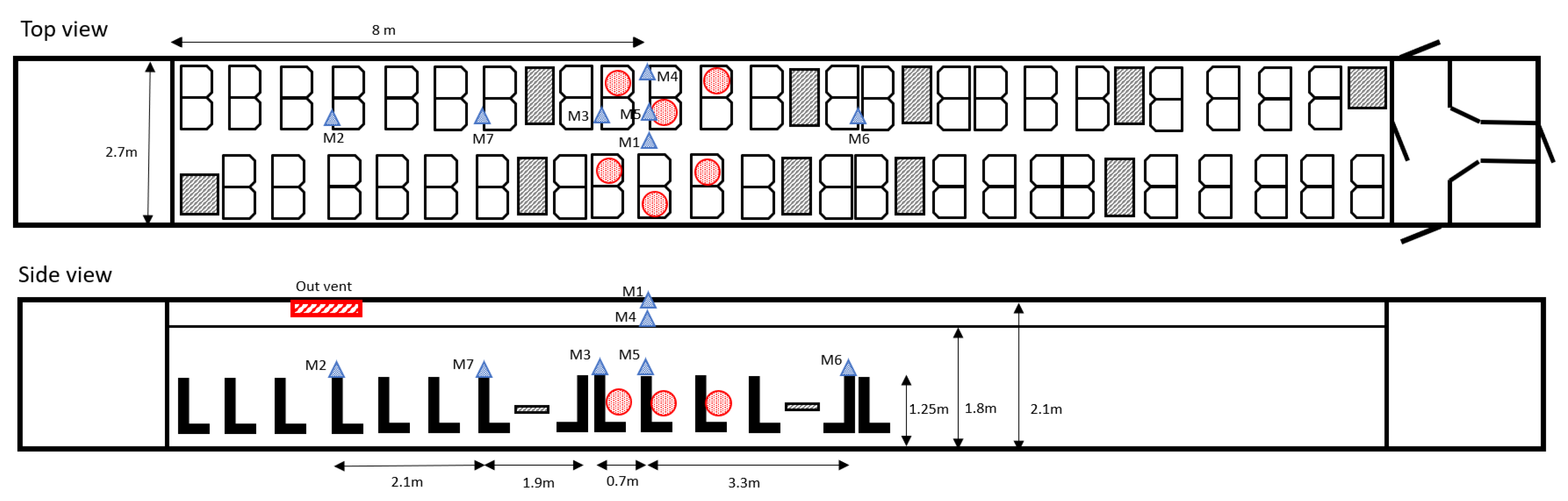
Figure 7 shows the CO${}_2$ measured by all sensors over the period beginning at the start of the first experiment and ending at the end of the last experiment. The figure includes uncontrolled periods in between experiments. The dashed lines indicate the beginning of each experiment when the ventilation was switched off, the time at which the ventilation was switched on, and the end of the experiment when the passengers were permitted to move from their seated positions. 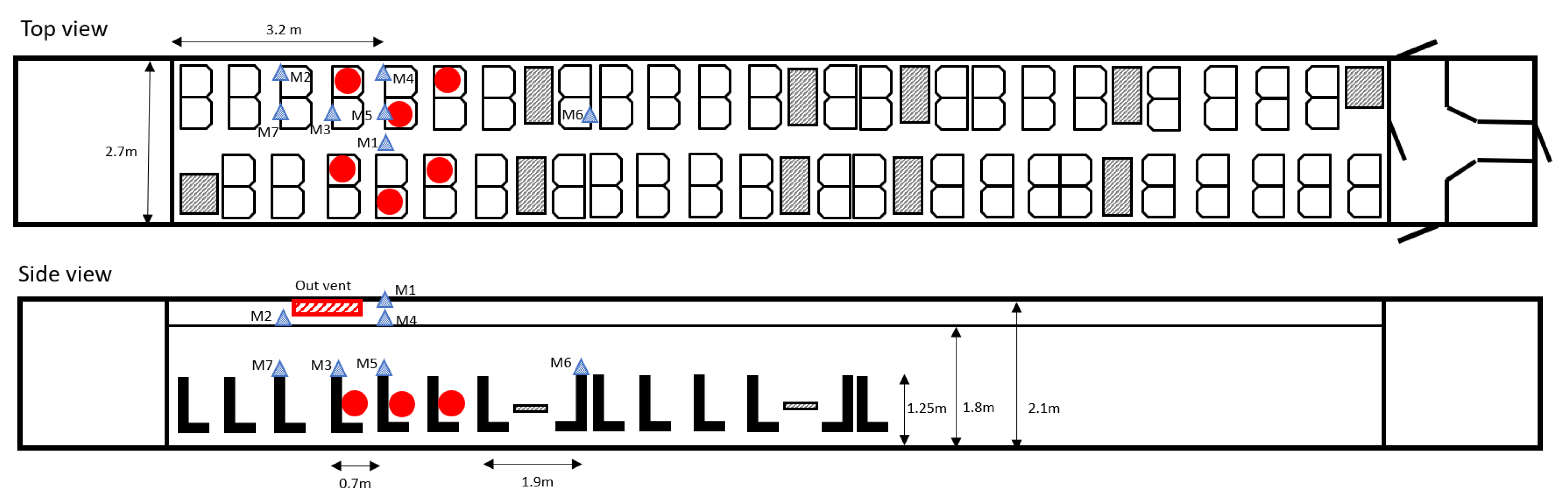The first two experiments, conducted before 1330, were at the middle of the saloon (Figure 3), while the second two experiments, after 1430, were at the end of the saloon (Figure 4).

The period of each experiment is evident from the increase in CO${}_2$ concentrations when the ventilation was switched off, followed by the rapid decrease in concentrations when the ventilation was switched on. These periods are also indicated by the dashed vertical lines. It is also evident that a steady-state was not reached at any point.

It is useful to see the data shortly before the beginning of each experiment as they highlight a limitation, which is that concentrations varied significantly between the start point of each experiment. No effort was made to control the period up to the beginning of each experiment. Therefore, the number of people present prior to each experimental run could vary in addition to the time period and ventilation setting used between each experiment, resulting in a variation in the initial CO${}_2$ concentrations at the beginning of each run. This variation is evident when considering the concentrations at the start of the first and second run for both the middle and end experiments. Concentrations were lower at the start of the second run in both cases as these began shortly after the period of forced ventilation from the first run, which resulted in a significant decrease in concentrations. These differences in initial conditions are reflected in the concentration trends observed during the experiments. For example, the rate of increase in CO${}_2$ was greater for the second run in both cases as the initial concentrations were lower. Despite the higher rate of increase, concentrations were generally still lower after 15 min, with no ventilation for the second runs.

A large decrease in concentrations was observed over the lunch period, between 1330 and 1420, during which time the saloon was empty, and the ventilation was set to automatic mode. At 1420, some people returned to the carriage and sat near the senors, from which point there was a sharp increase in concentrations. The maximum number of people in the saloon at any given time was six.

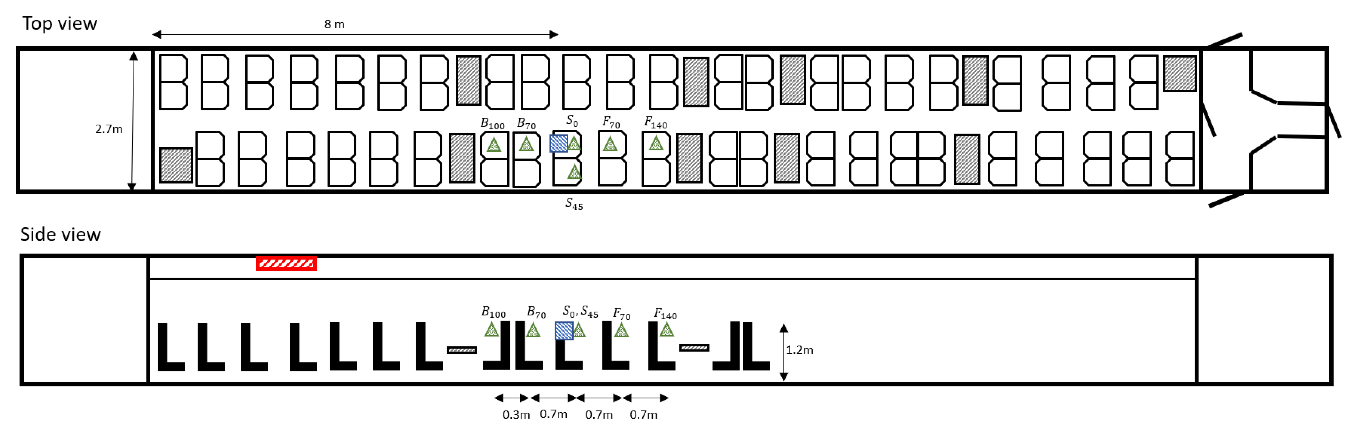
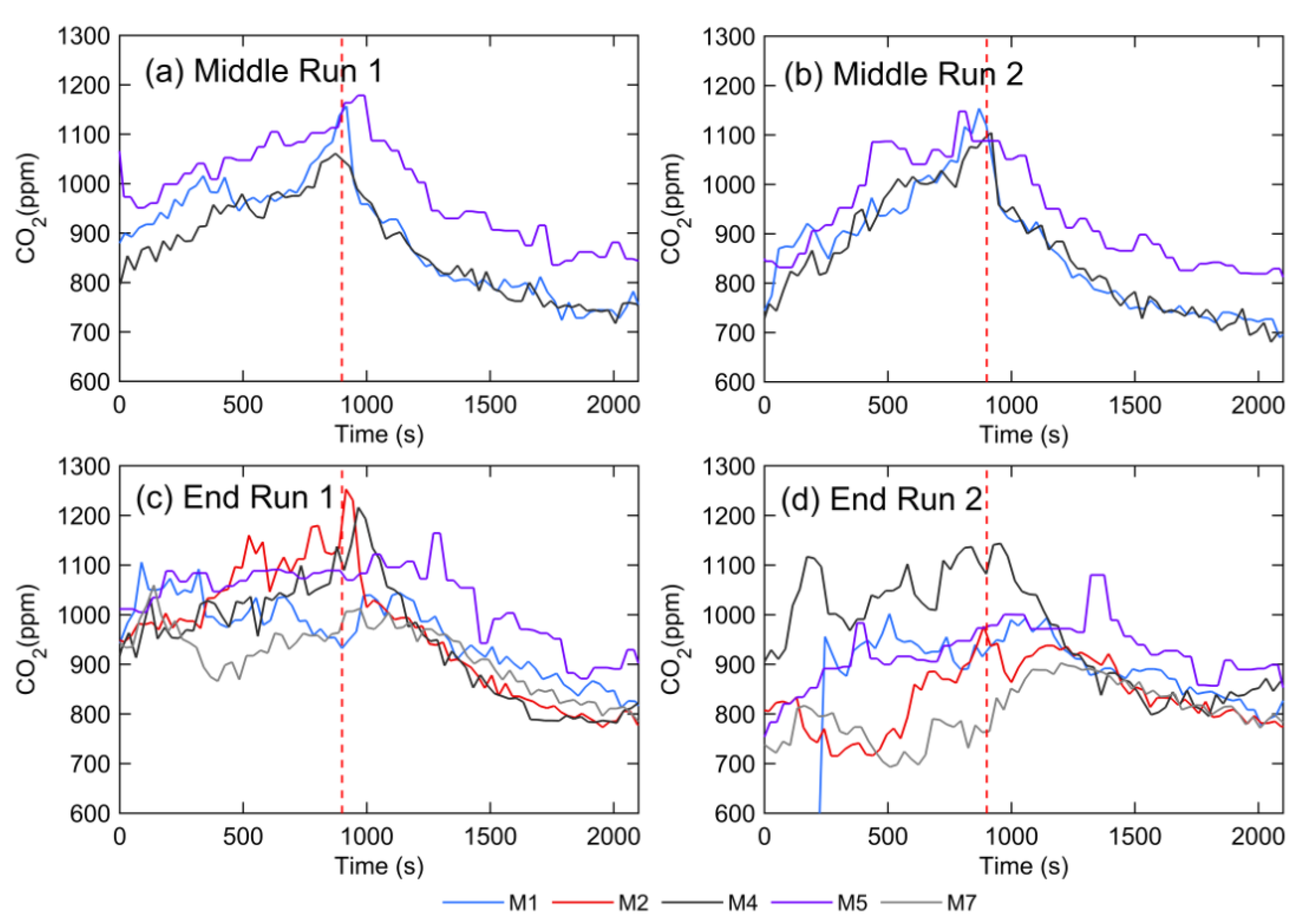
Figure 8 shows the concentrations for the sensors placed at breathing zone height for sitting passengers. The highest concentrations were generally observed for M5 located between two rows of passengers, with the concentrations here consistently above those at M7 and M3. The distance between M3 and M5 is 0.8 m. Once ventilation was switched on at 900 s (15 min), the concentrations began to decrease at each location. The rate of decrease was highest for M6 (the sensor furthest from the nearest extract vent) for all experiment runs. For the experiment at the middle of the saloon, a much lower rate of decay was observed for M2 (the sensor closest to the nearest extract vent) despite being located further from the CO${}_2$ source. In fact, for the first run, an increase in concentrations was observed for M2. This suggests that the CO${}_2$ generated by the passengers travelled towards the nearest extract vent, shown in Figure 3 and Figure 4; when the ventilation was switched on, the elevated CO${}_2$ at M6 quickly diluted, while the reduction due to dilution at M2 was countered by elevated concentrations advected by air flow from the direction of the passengers. The rates of decay for the M3, M5, and M7 sensors are higher at the middle of the carriage than compared to the end. This suggests that the effective ventilation rate is higher at the middle of the carriage, at least initially.

Figure 9 shows the concentrations for sensors placed at different heights at the same location along the length of the saloon. For the experiment at the middle of the carriage, this constituted M1 (ceiling), M4 (luggage rack), and M5 (breathing zone) only. Here, no significant difference was observed between M1 and M4, however, M5 showed consistently higher concentrations. A similar picture was observed for M1, M4, and M5 at the end of the saloon. At the end of the saloon, M2 was located directly above M7. In this case, M2 showed higher concentrations than M7, indicating that there may be stratification during the unventilated period. Once the ventilation was switched on, the concentrations at the two locations quickly converged, suggesting that the ventilation was effective at mixing the air vertically.

The steady-state was not reached for these experiments; threrefore, we were unable to draw firm conclusions based on the absolute differences in concentrations between locations as it was unclear to what extent these differences would have converged given sufficient time. However, it seems likely that the concentration at certain locations would have remained higher than others. For example, it is likely that the steady-state concentration for M6 would have been significantly lower than for all other sensors based on the trends observed in Figure 8. This suggests that the saloon was not well mixed along its length despite the supply of recirculated air throughout the saloon, but it was well mixed over its height.

3.2. Aerosol Dispersion

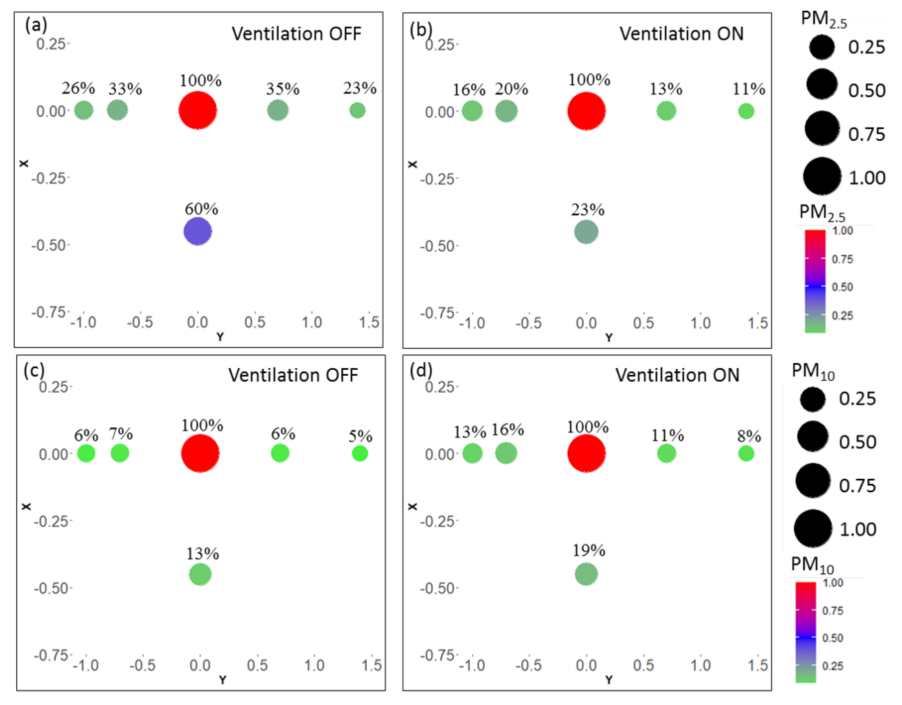
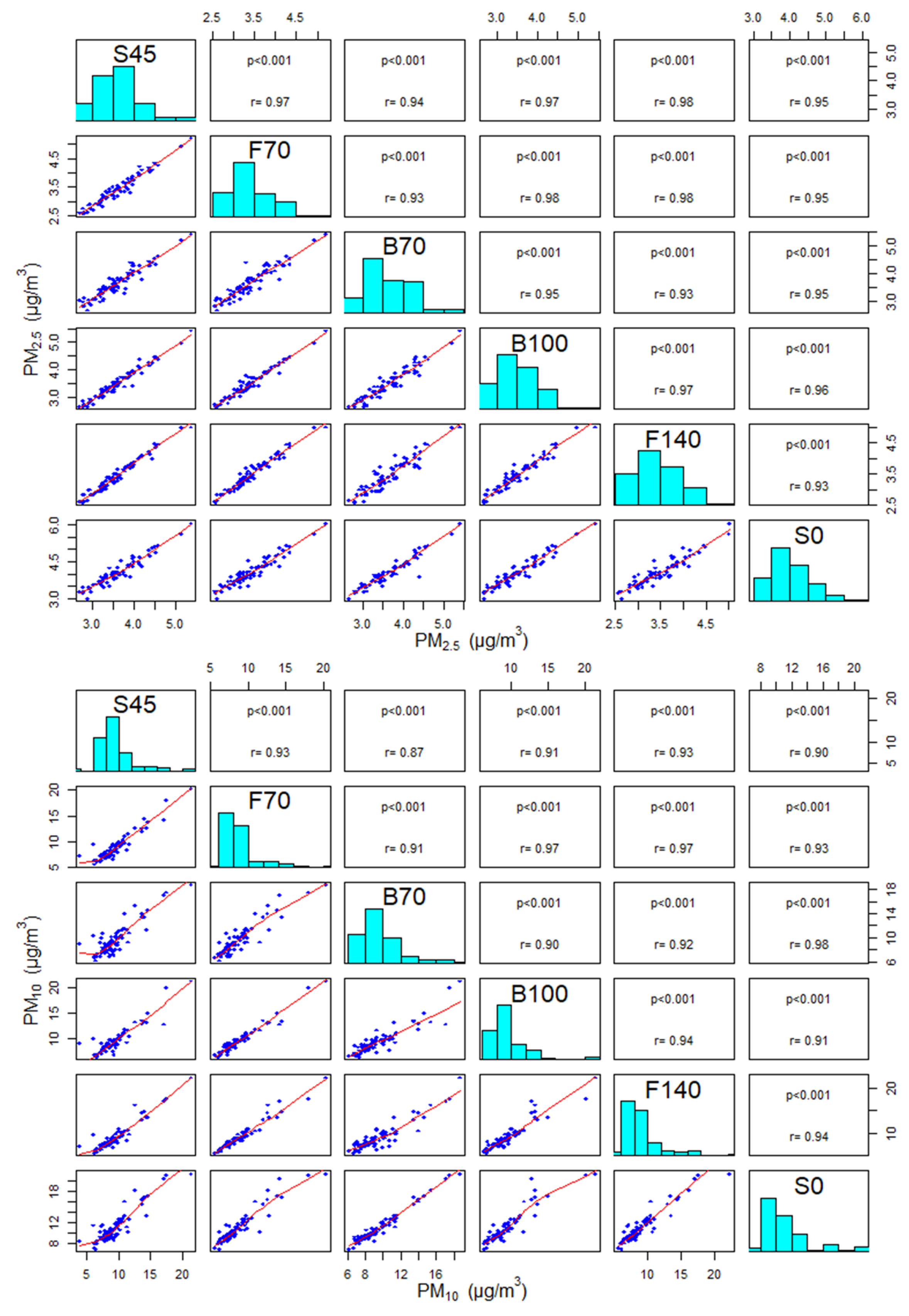
Figure 10 shows the normalised mean concentrations measured for the aerosol released from the nebuliser during the ventilation off and on periods at each location. During the unventilated period, the ${\mathrm{PM}}_{10}$ concentration dropped off very quickly from the source location by a factor of nearly nine between $S_0$ and the next nearest monitor, $S_{45}$. The relative decrease was much greater than that observed for ${\mathrm{PM}}_{2.5}$ concentrations, which decreased by 40% between these two locations. This highlights the difference in the dispersion of the smaller and larger particles. During this unventilated period, there were no advective flows present within the carriage, and the dilution of the aerosol occurs due to diffusion and small scale turbulent mixing. Due to their greater mass, the larger aerosol particles are not dispersed as effectively as the smaller particles under these conditions. The low relative humidity in the carriage and the use of salt solution to generate the aerosols will have resulted in evaporation, resulting in a decrease in droplet size, which will also have contributed to the difference observed between the size fractions as some of the initially larger droplets reduced in size and became attributed to the smaller size fraction.

Switing on the ventilation resulted in a significant reduction in concentrations at all locations (see

Table A1. Mean and standard deviation concentrations ($\mathsf{\mu }$ g m${}^{-3}$) of fine and coarse aerosol concentrations and normalised concentrations at different distances from the source under ventilation off and on conditions.

	${\mathit{S}}_0$	${\mathit{B}}_{100}$	${\mathit{B}}_{70}$	${\mathit{S}}_{45}$	${\mathit{F}}_{70}$	${\mathit{F}}_{140}$
${\mathrm{PM}}_{10}$ Off	1701 ± 511.9	77 ± 16	91 ± 19	194 ± 45	88 ± 18	66 ±  18
$C_{norm}(\%)$	100	6	7	13	6	5
${\mathrm{PM}}_{10}$ On	483 ± 134	48 ± 7	61 ± 10	74 ± 18	39 ± 6	31 ± 3
$C_{norm}(\%)$	100	13	16	19	11	8
${\mathrm{PM}}_{2.5}$ Off	369 ± 216	55 ± 12	65 ± 14	143 ± 34	67 ± 14	49 ± 13
$C_{norm}(\%)$	100	26	33	60	35	23
${\mathrm{PM}}_{2.5}$ On	283 ± 67	38 ± 6	48 ± 8	58 ± 14	32 ± 5	25 ± 3
$C_{norm}(\%)$	100	16	20	23	13	11

); mixing was increased due to advection and increased turbulence within the carriage. The largest relative decrease of 72% was observed at $S_0$ for the coarse aerosol, highlighting the effectiveness of the ventilation in driving the dilution of these larger particles. However, the normalised concentrations of the fine particles remained greater than those of the coarse particles at each location away from the source, indicating the more effective mixing of the finer fraction.

When the ventilation was switched on, higher concentrations were observed for both the coarse and fine fraction in the “backward” direction than compared to the “forward” direction. This suggests that the prevailing flow was directed in the “backwards” direction. This was the direction towards the nearest extract vent in the saloon, as also observed from the CO${}_2$ measurements.

Finally, the concentrations at $S_{45}$, which was located at the seat next to the source, were only marginally greater than those at $B_{70}$ located on the next row. This suggests that, over these short length scales, the degree of mixing across the width of the saloon was similar to that along its length.

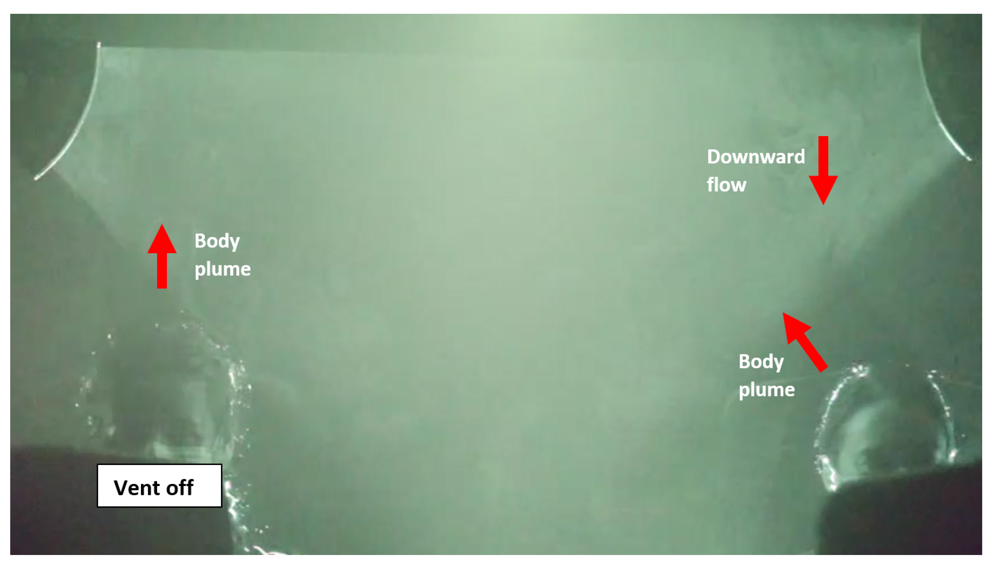
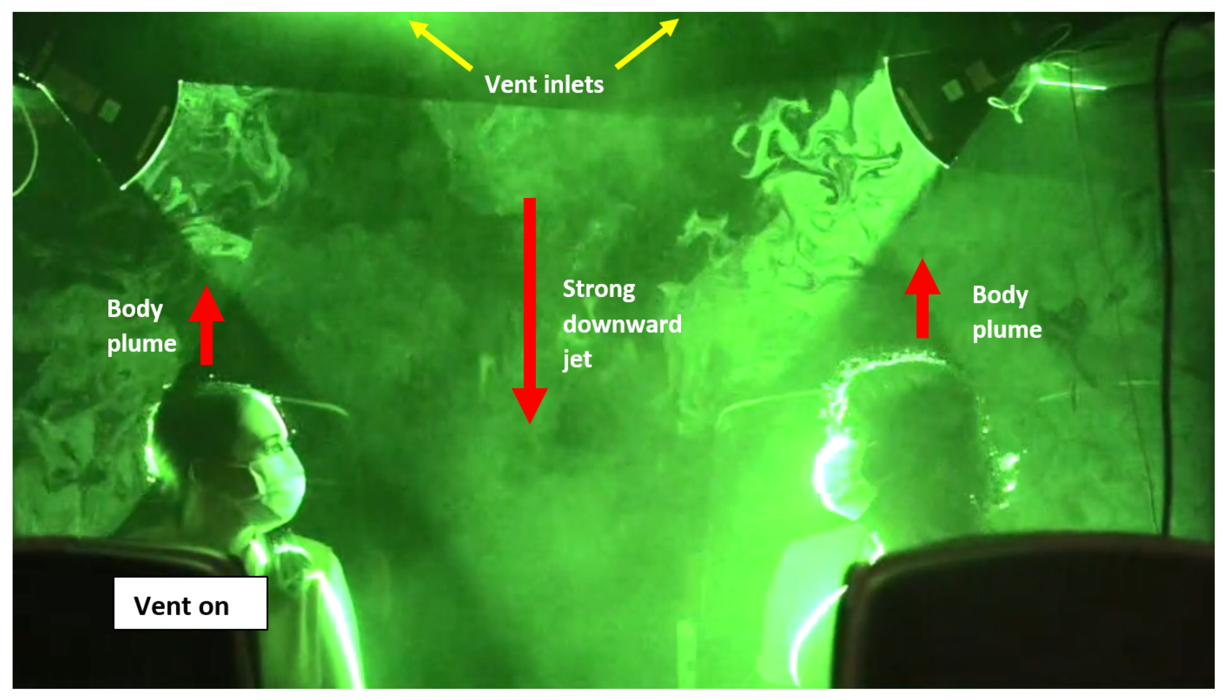
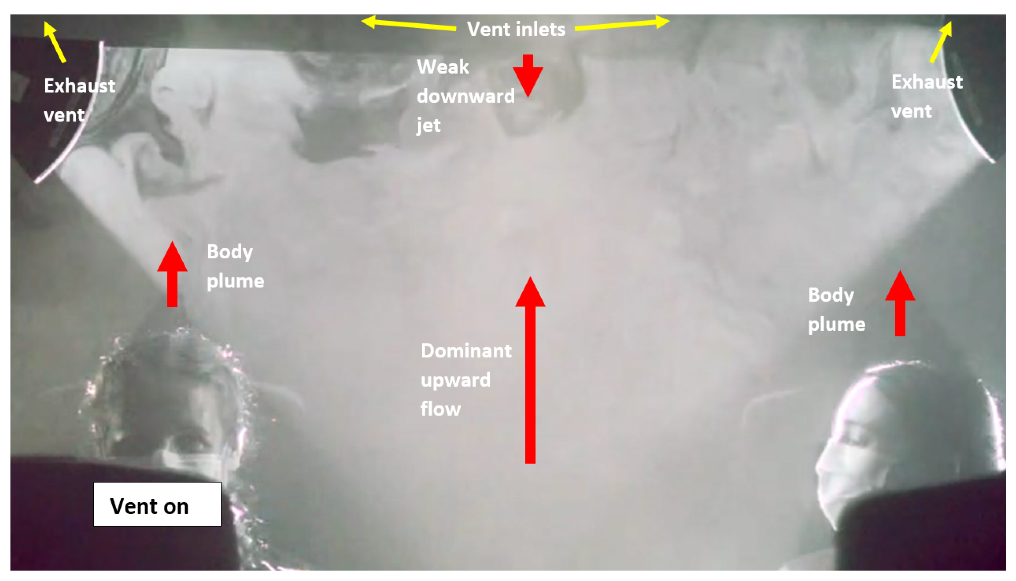
3.3. Flow Visualisation

Figure 11, Figure 12, Figure 13 and Figure 14 show still images of the flow visualisation experiment at the middle and end of the carriage, respectively. Red arrows are used to indicate the direction of persistent air flow. Videos of these flow visualisations are available in the Supplementary Materials for which the airflow patterns are clearer.

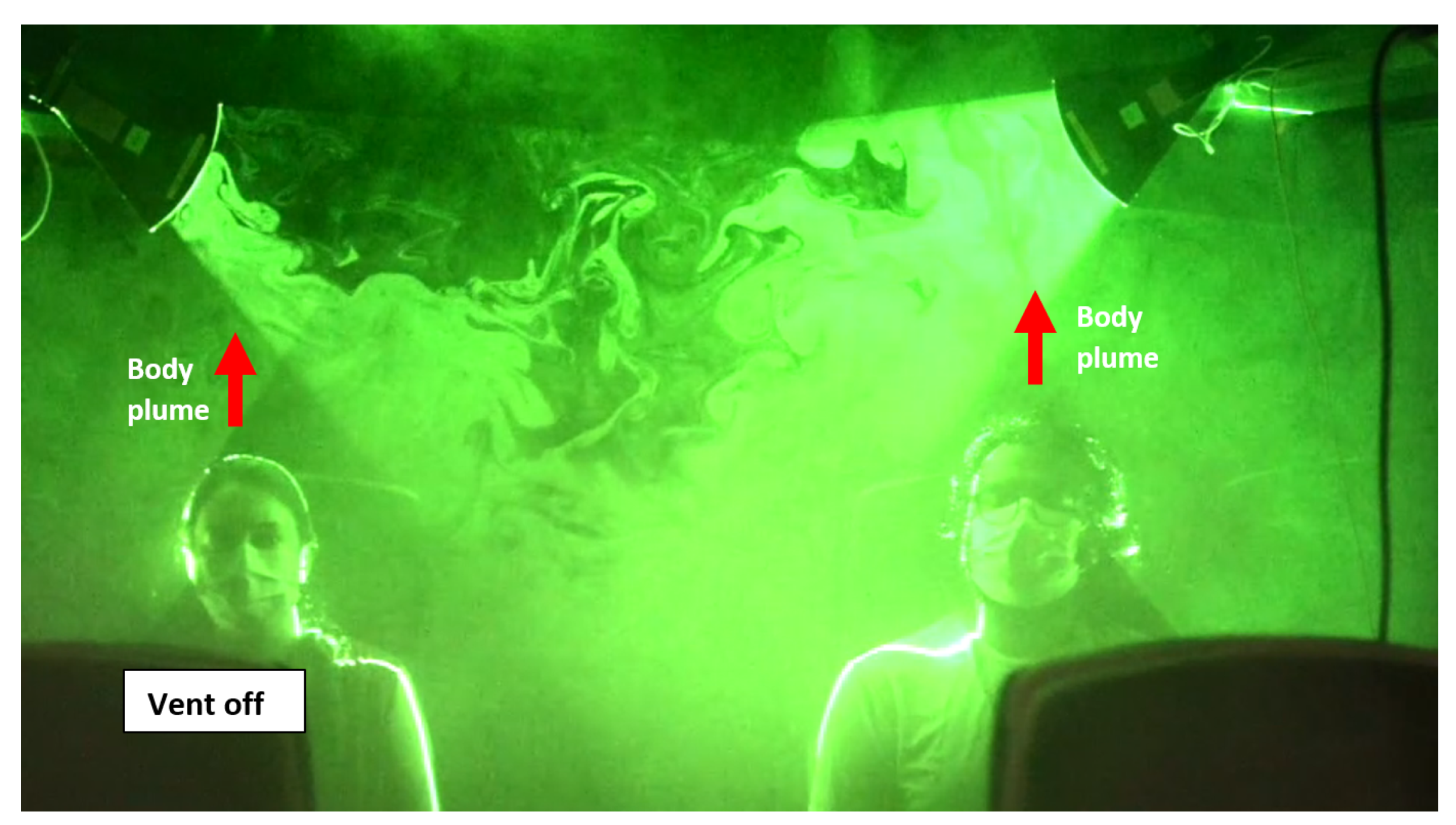
During the unventilated period, the body plumes rising from the two passengers are clearly visible in the video footage for both the middle and end cases. In the middle of the carriage, there were no other persistent flows present other than some turbulent mixing. At the end of the carriage, there was a weak but persistent downward flow from the ceiling above the passenger on the right. This flow in turn forced the body plume from the passenger on the right to rise at an angle towards the centre of the carriage. This downward flow may have been due to an asymmetry in the body plumes generated by the two passengers.

In the middle of the carriage, when the ventilation was switched on, a strong downward jet was observed to flow from the ceiling inlet vents (Figure 2). This downward flow was sufficiently strong to extend between the two passengers and beyond the lower edge of the image, acting as an air curtain between the passengers. The body plumes rising from the two passengers continued to drive an upward flow while the ventilation was switched on, causing significant upward acceleration.

At the end of the carriage, when the ventilation was switched on, the flow patterns were very different compared to those observed in the middle of the carriage. In this case, only a very weak downward jet was observed to flow from the inlet vents, extending only a few centimetres into the space, while a persistent upward flow was observed across the remaining cross section of the carriage. In this case, the passengers were sat directly below the extract vents. The dominant upward flow is driven by the suction of these vents.

4. Discussion

Given that only six people were used for the CO${}_2$ experiments, relatively high concentrations were measured in the carriage. While the steady-state was not reached during the CO${}_2$ experiments, it is clear from Figure 8 and Figure 9 that concentrations near the passengers (M3, M5, and M7) converge towards a value of around 800 ppm. Given that the carriage has a seated occupancy of 88, the concentrations are likely to be considerably higher in a busy carriage. CIBSE recommends an outdoor air flow rate for buildings of 10 L s${}^{-1}$ person${}^{-1}$ (Ls${}^{-1}$p${}^{-1}$) [40]. When achieved, this ensures that CO${}_2$ concentrations are unlikely to exceed 1000 pmmin a well-mixed space (concentrations above which have been related to adverse health impacts [41]). The ventilation flow rate was not known for these experiments, and it is not clear how the provision of fresh air provided by the 75% forced cooling setting used for these experiments compares with that provided by the automatic function of the ventilation system during normal service. 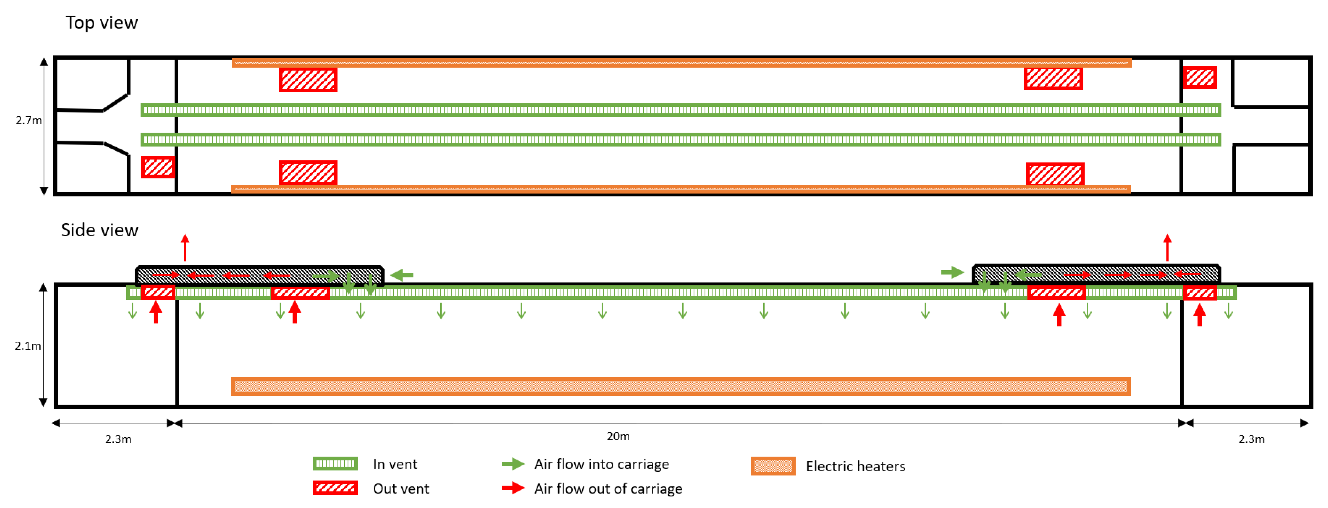While ventilation rates can be estimated from CO${}_2$ decay curves or steady-state concentrations (e.g., [42]), these estimates depend on a well mixed assumption, which is not the case for the CO${}_2$ experiments here. However, the design specification of the HVAC system placed the minimum and maximum ventilation rates, that is, the rate of supply of fresh air, at 22.5–30 m${}^3$ min${}^{-1}$. During normal operation, the exact rate varies within these limits in response to temperature senors; however, the system does not react directly to the occupancy of the carriage. Taking the carriage volume of 140 m${}^3$, this equates to 9.6–12.9 air changes per hour (ACH). If we assume a carriage at half seating occupancy, holding 44 passengers, this works out as 8.5 to 11.4 Ls${}^{-1}$p${}^{-1}$. For a carriage at full seating occupancy, these values will be halved. In a recent review by the National Engineering Policy Centre (NEPC), values as low as 4 to 6 ACH were given for the provision of outdoor air to certain UK rail carriages [43]. Assuming the same carriage volume of 140 m${}^3$ and an occupancy of 44 passengers, this works out as 3.5 to 5.3 Ls${}^{-1}$p${}^{-1}$, which is significantly lower than that recommended by CIBSE for buildings, but comparable to the ASHRAE recommended flow rates for commercial aircraft of 3.5 Ls${}^{-1}$p${}^{-1}$ (ASHRAE Standard 161). However, for a busy carriage, the air flow rate per person will be significantly lower.

Train carriages are not required to meet the same ventilation standards as indoor spaces in buildings. Ventilation systems on train carriages tend to be optimised for energy efficiency and passenger comfort rather than air quality. To minimise the energy consumption of HVAC systems on trains, much of the air supply is recirculated air rather than outdoor air that usually requires a higher degree of heating or cooling in order to maintain passenger comfort. The provision of outdoor air by these HVAC systems can, therefore, be low, and the recirculation of air could result in the dispersion of virus-laden particles throughout the space. While the recirculated air will be passed through a filter within the HVAC unit, most filters are too coarse to remove smaller viral particles [44]. Unlike aircraft, which are fitted with High Efficiency Particle Arrestance (HEPA) filters [28], this is not a requirement for train carriages. It is not clear from the experiments performed in this study what effect the recirculation of air has on the risk of transmission. For trains, European Union (EU) regulations and those adopted by the UK’s Rail Safety and Standards Board specify that CO${}_2$ concentrations should not exceed 5000 ppm (EU regulation No 1302/2014); however, there are no further requirements regarding indoor air quality. Given that CO${}_2$ concentrations, together with the occupancy and HVAC filter efficiency, can be directly related to the risk of airborne transmission [11,12,13], the absence of more stringent regulations may be a cause for concern in terms of mitigating airborne transmission in addition to general air quality considerations. Further investigation is required to determine the efficacy of the HVAC filter in removing viral-laden particles from the air.

Within the context of the current COVID-19 pandemic, it should be noted that the risk of airborne transmission relative to that via droplets or contaminated surfaces is still not well understood. However, it is by now clear that airborne transmission is a significant component, as is now acknowledged by the World Health Organization [45]. The degree to which increasing the fresh air supply rate within a space reduces the risk of airborne transmission depends on the airflow structures within the space [46], the main factor being what proportion of the additional fresh air supplied reaches the breathing zone. However, given the experiments presented here suggesting that the carriage is well mixed along the vertical direction, it is likely that an increase in fresh air supply will result in a reduction in transmission risk. To what extent and whether adjusting the ventilation rates is a sensible measure remain outstanding questions that require further research. Train operators in the UK have taken practical measures currently available towards minimising the risk to passengers while travelling during the pandemic. These measures include the use of antimicrobial surface treatment, encouraging passengers to sit as far as possible from others, and enforcing mask wearing at all times. Furthermore, the risk of airborne transmission is limited by the short time periods typically spent in train carriages relative to other environments, for example, in buildings. It is also worth noting that public transport will, on the whole, have lower viral emission risk factors as most people tend to be passive while travelling rather than talking or exercising, which increase viral emissions considerably [47]. For these reasons, while we have compared the fresh air supply rates on train carriages to those recommended for buildings to provide context, we are not necessarily suggesting that equivalent rates are necessary or practical for train carriages. It is also for these reasons that the risk of infection on an individual basis on a train carriage is likely to be low. However, given the large number of passengers who travel by rail every day, the contribution to the population level “R” rate may be significant and justifies further investigation.

The experiments revealed the complexity of the airflow patterns and, therefore, the dispersion of particles within the carriage saloon. Significant differences were observed in the CO${}_2$ concentrations within the saloon along its length. Therefore, we can conclude that the air within the saloon is not well mixed along its length, at least not while the train is stationary or while travelling at steady speed. Maximising the physical distance between passengers along the length of the carriage is, therefore, likely to be an effective strategy at reducing the risk of airborne transmission. A downward jet observed in the flow visualisation at the middle of the saloon may act as an air curtain along the aisle; however, the aerosol concentrations measured at $S_{45}$ were similar to those measured on the row behind the source. This suggests a similar degree of mixing in both directions in the absence of passengers. therefore, it seems that, in the case of a busy carriage where physical distancing is not possible, there is not much of advantage to either sitting across the aisle on the same row or sitting one row ahead of or behind another passenger.

The ventilation seemed effective at removing any stratification of CO${}_2$ concentrations; therefore, it may be appropriate to consider the saloon as well mixed throughout its height. The airflow visualisations also demonstrated the importance of considering the convective plumes generated by the body heat of the passengers. These were clearly visible both when ventilation was on and off and may have a significant effect on the initial trajectory of exhaled droplets in addition to the general flow patterns within the saloon, particularly when occupancy is high. The experiments also demonstrate the sensitivity of the airflow to the location of the extract vents. Both the CO${}_2$ and aerosol particle dispersion experiments showed a strong bias in dispersion towards the nearest extract vent. Furthermore, significantly different flow patterns were observed at the end and middle of the saloon. The dominant upward flow observed at the end of the saloon is due to the suction of the extract vents that were positioned directly above. The different flow behaviour between the middle and end of the saloon, along with the large differences in CO${}_2$ measured along its length, suggests that the risk of airborne transmission may vary depending on the seating positions of the passengers and the location of any infected passenger.

The aerosol dispersion experiments demonstrated the importance of considering particle size or mass. Measurements suggested a slightly higher degree of dilution for the fine fraction of particles than for the coarse fraction; however, both size fractions were dispersed effectively. This, along with the large decrease in CO${}_2$ measured with distance from passengers, suggests that physical distancing, where possible, is likely to be an effective strategy for reducing the risk of airborne transmission, particularly from larger droplets. The size and mass of viral-laden droplets can cover a wide range [35]. Therefore, it is important to understand the dispersion behaviour for the full range of exhaled droplet sizes (0.01–1000 $\mathsf{\mu }$m). In these experiments, only the difference between two size ranges was considered. Ideally, a more advanced particle counter would be used to achieve insight into a broader range of particle sizes. Furthermore, while CO${}_2$ is a useful indicator of exhaled air, its measurements do not provide insight into dispersion of larger droplets.

There are several limitations to the experiments presented here. First, only a limited number of runs were performed for each experimental method. Second, it was not always possible to allow sufficient time to reach a steady-state during and in between experiments. These limitations were due to the short time period available on the train. Finally, as the experiments took place during the COVID-19 pandemic, the time spent on the carriage was limited in order to mitigate the risk of transmission between those undertaking the experiments.

Despite these factors, the utility of the methods used has been demonstrated for full scale experiments. They have also shown the complexity of the airflow within an intercity train carriage and have provided some useful insights into flow behaviour within the saloon. It is clear that simple approaches such as using the Wells–Riley equation [48], which assumes a well-mixed space, are unlikely to provide accurate estimates of the probability of infection. It is also worth noting that an intercity carriage is likely to represent the simplest case in relation to airflow and droplet dispersion. In this case, journey times tend be longer; therefore, passengers are more likely to remain seated for longer periods of time, there are fewer occurrences of boarding and alighting, and the carriage doors do not open directly into the saloon. This is not the case for regional trains in which the increase in people’s movement, increase in the frequency of stops, carriage accelerations, and decelerations in addition to the exchange of air when doors are opened are likely to significantly increase the complexity of the problem. In order to fully understand the implications of these insights to the risk of airborne transmission in addition to their relevance for different ventilation settings and carriage occupancy, a high fidelity model such as CFD may be required. The data gathered here will prove useful for comparison with and provide confidence in future CFD simulations. Furthermore, the experiments have provided useful insights for the development of a 1D advection–diffusion model which is currently work in progress. An alternative approach for understanding the risk of airborne transmission on the carriage is to deploy CO₂ sensors within the carriage while in service; the measurements can be used to estimate transmission risk [13].

5. Conclusions

The experiments presented in this paper were performed at short notice and during somewhat challenging conditions during the COVID-19 pandemic (during the August of 2020). Therefore, they do not represent a comprehensive analysis of the airborne transmission on the carriage; nevertheless, they are a rare example of experiments conducted at full-scale on an operational train carriage. Three experiments were performed on a stationary intercity train carriage using a single ventilation setting (75% forced cooling). The data obtained consisted of CO${}_2$ measurements of exhaled air, measurements of aerosol particles from a nebuliser, and flow visualisations of fog illuminated using lasers. All three experiments were successful in providing useful insights into the flow and dispersion behaviour on the carriage and also demonstrated the “proof of concept” for these methods for full-scale experiments. For example, it was found that the carriage saloon is not well mixed along its length; however, it is likely to be well mixed along its height and width. This is useful information for the rail operator when considering suitable seating restrictions to enforce physical distancing. Based on the findings reported here, it is recommended that in order to mitigate the risk of airborne transmission, mask wearing should be encouraged on intercity train carriages, and any practical measures available to encourage physical distancing between passengers during periods of low occupancy should be implemented. While some of the insights may seem intuitive, there is value in their verification. These findings will inform further experiments that are planned.

The suitability of the fresh air supply rates on UK train carriages is also discussed by drawing on the CO₂ concentrations measured during these experiments.

References

1. DfT. Transport Use by Mode: Great Britain, Since 1 March 2020. 2020. Available online: https://www.gov.uk/government/statistics/transport-use-during-the-coronavirus-covid-19-pandemic (accessed on 23 September 2020).
2. The Royal Society. Face Masks for the General Public | Royal Society DELVE Initiative; The Royal Society: London, UK, 2020. [Google Scholar]
3. Burridge, H.C.; Bhagat, R.K.; Stettler, M.E.J.; Kumar, P.; De Mel, I.; Demis, P.; Hart, A.; Johnson-Llambias, Y.; Felipe King, M.; Klymenko, O.; et al. The ventilation of buildings and other mitigating measures for COVID-19: A focus on wintertime. Proc. R. Soc. A 2021, 477, 20200855. [Google Scholar] [CrossRef]
4. Morawska, L.; Tang, J.W.; Bahnfleth, W.; Bluyssen, P.M.; Boerstra, A.; Buonanno, G.; Cao, J.; Dancer, S.; Floto, A.; Franchimon, F.; et al. How can airborne transmission of COVID-19 indoors be minimised? Environ. Int. 2020, 142, 105832. [Google Scholar] [CrossRef]
5. Morawska, L.; Cao, J. Airborne transmission of SARS-CoV-2: The world should face the reality. Environ. Int. 2020, 139, 105730. [Google Scholar] [CrossRef] [PubMed]
6. Mittal, R.; Ni, R.; Seo, J.H. The flow physics of COVID-19. J. Fluid Mech. 2020, 894. [Google Scholar] [CrossRef]
7. Bourouiba, L.; Dehandschoewercker, E.; Bush, J. Violent expiratory events: On coughing and sneezing. J. Fluid Mech. 2014, 745, 537–563. [Google Scholar] [CrossRef]
8. Lindsley, W.G.; Noti, J.D.; Blachere, F.M.; Szalajda, J.V.; Beezhold, D.H. Efficacy of face shields against cough aerosol droplets from a cough simulator. J. Occup. Environ. Hyg. 2014, 11, 509–518. [Google Scholar] [CrossRef] [PubMed]
9. Van Doremalen, N.; Bushmaker, T.; Morris, D.H.; Holbrook, M.G.; Gamble, A.; Williamson, B.N.; Tamin, A.; Harcourt, J.L.; Thornburg, N.J.; Gerber, S.I.; et al. Aerosol and surface stability of SARS-CoV-2 as compared with SARS-CoV-1. N. Engl. J. Med. 2020, 382, 1564–1567. [Google Scholar] [CrossRef] [PubMed]
10. Kumar, P.; Morawska, L. Could fighting airborne transmission be the next line of defence against COVID-19 spread? City Environ. Interact. 2019, 4, 100033. [Google Scholar] [CrossRef]
11. Rudnick, S.N.; Milton, D.K. Risk of indoor airborne infection transmission estimated from carbon dioxide concentration. Indoor Air 2003, 13, 237–245. [Google Scholar] [CrossRef]
12. Vouriot, C.V.M.; Burridge, H.C.; Noakes, C.J.; Linden, P.F. Seasonal variation in airborne infection risk in schools due to changes in ventilation inferred from monitored carbon dioxide. Indoor Air 2021. [Google Scholar] [CrossRef]
13. Burridge, H.C.; Fan, S.; Jones, R.L.; Noakes, C.J.; Linden, P.F. Predictive and retrospective modelling of airborne infection risk using monitored carbon dioxide. Indoor Built Environ. 2021, accept. [Google Scholar] [CrossRef]
14. Conceição, E.Z.; Silva, M.C.; Viegas, D.X. Airflow Around a Passenger Seated in a Bus. HVAC R Res. 1997, 3, 311–323. [Google Scholar] [CrossRef]
15. Conceicao, E.; Silva, M.; Viegas, D. Evaluation of the thermal comfort level perceived by a passenger in a bus compartment. In Proceedings of the Fifth International Conference on Air Distribution in Rooms, ROOMVENT, Yokohama, Japan, 17–19 July 1996; Volume 96, pp. 403–413. [Google Scholar]
16. Li, J.; Cao, X.; Liu, J.; Mohanarangam, K.; Yang, W. PIV measurement of human thermal convection flow in a simplified vehicle cabin. Build. Environ. 2018, 144, 305–315. [Google Scholar] [CrossRef]
17. Pawar, S.; Gade, U.R.; Dixit, A.; Tadigadapa, S.B.; Jaybhay, S. Evaluation of Cabin Comfort in Air Conditioned Buses Using CFD. In Proceedings of the SAE 2014 World Congress & Exhibition, Detroit, MI, USA, 8–10 April 2014. [Google Scholar] [CrossRef]
18. Konstantinov, M.; Wagner, C. Numerical Simulation of the Thermal Comfort in a Train Cabin. Int. J. Railw. Technol. 2015, 4, 69–88. [Google Scholar] [CrossRef]
19. Yang, L.; Li, X.; Tu, J. Thermal comfort analysis of a high-speed train cabin considering the solar radiation effects. Indoor Built Environ. 2020, 29, 1101–1117. [Google Scholar] [CrossRef]
20. Mingotti, N.; Wood, R.; Noakes, C.; Woods, A.W. The mixing of airborne contaminants by the repeated passage of people along a corridor. J. Fluid Mech. 2020, 903, A52. [Google Scholar] [CrossRef]
21. Wang, H.; Lin, M.; Chen, Y. Performance evaluation of air distribution systems in three different China railway high-speed train cabins using numerical simulations. Build. Simul. 2019, 7, 629–638. [Google Scholar] [CrossRef]
22. Zhang, L.; Li, Y. Dispersion of coughed droplets in a fully-occupied high-speed rail cabin. Build. Environ. 2012, 47, 58–66. [Google Scholar] [CrossRef]
23. Yang, X.; Ou, C.; Yang, H.; Liu, L.; Song, T.; Kang, M.; Lin, H.; Hang, J. Transmission of pathogen-laden expiratory droplets in a coach bus. J. Hazard. Mater. 2020, 397, 122609. [Google Scholar] [CrossRef]
24. Zhu, S.; Srebric, J.; Spengler, J.D.; Demokritou, P. An advanced numerical model for the assessment of airborne transmission of influenza in bus microenvironments. Build. Environ. 2012, 47, 67–75. [Google Scholar] [CrossRef]
25. Olsen, S.J.; Chang, H.L.; Cheung, T.Y.Y.; Tang, A.F.Y.; Fisk, T.L.; Ooi, S.P.L.; Kuo, H.W.; Jiang, D.D.S.; Chen, K.T.; Lando, J.; et al. Transmission of the Severe Acute Respiratory Syndrome on Aircraft. N. Engl. J. Med. 2003, 349, 2416–2422. [Google Scholar] [CrossRef] [PubMed]
26. Yan, W.; Zhang, Y.; Sun, Y.; Li, D. Experimental and CFD study of unsteady airborne pollutant transport within an aircraft cabin mock-up. Build. Environ. 2009, 44, 34–43. [Google Scholar] [CrossRef]
27. Mazumdar, S.; Chen, Q. A one-dimensional analytical model for airborne contaminant transport in airliner cabins. Indoor Air 2009, 19, 3–13. [Google Scholar] [CrossRef]
28. Elmaghraby, H.A.; Chiang, Y.W.; Aliabadi, A.A. Ventilation strategies and air quality management in passenger aircraft cabins: A review of experimental approaches and numerical simulations. Sci. Technol. Built Environ. 2018, 24, 160–175. [Google Scholar] [CrossRef]
29. Ryan, P.; Spengler, J.D.; Halfpenny, P.F. Sequential box models for indoor air quality: Application to airliner cabin air quality. Atmos. Environ. 1988, 22, 1031–1038. [Google Scholar] [CrossRef]
30. Ko, G.; Thompson, K.M.; Nardell, E.A. Estimation of Tuberculosis Risk on a Commercial Airliner. Risk Anal. 2004, 24, 379–388. [Google Scholar] [CrossRef] [PubMed]
31. Silcott, D.; Kinahan, S.; Santarpia, J.; Silcott, R.; Silcott, P.; Silcott, B.; Distelhorst, S.; Herrera, V.; Rivera, D.; Crown, K.; et al. TRANSCOM/AMC Commercial Aircraft Cabin Aerosol Dispersion Tests; United States Transportation Command (USTRANSCOM): Belleville, IL, USA; Air Mobility Command (AMC): Scott Air Force Base, IL, USA, 2020. [Google Scholar]
32. Elmaghraby, H.A.; Chiang, Y.W.; Aliabadi, A.A. Are aircraft acceleration-induced body forces effective on contaminant dispersion in passenger aircraft cabins? Sci. Technol. Built Environ. 2019, 25, 858–872. [Google Scholar] [CrossRef]
33. Elmaghraby, H.A.; Chiang, Y.W.; Aliabadi, A.A. Airflow design and source control strategies for reducing airborne contaminant exposure in passenger aircraft cabins during the climb leg. Sci. Technol. Built Environ. 2020, 26, 901–923. [Google Scholar] [CrossRef]
34. Elmaghraby, H.A.; Chiang, Y.W.; Aliabadi, A.A. Normal and extreme aircraft accelerations and the effects on exposure to expiratory airborne contaminant inside commercial aircraft cabins. Sci. Technol. Built Environ. 2020, 26, 924–927. [Google Scholar] [CrossRef]
35. Bake, B.; Larsson, P.; Ljungkvist, G.; Ljungström, E.; Olin, A. Exhaled particles and small airways. Respir. Res. 2019, 8. [Google Scholar] [CrossRef] [Green Version]
36. Kannan, R. Breathing Rates and Breathing Air Constituents. Int. J. Innov. Sci. Eng. Technol. 2015, 2, 557–558. [Google Scholar]
37. Kumar, P.; Rivas, I.; Sachdeva, L. Exposure of in-pram babies to airborne particles during morning drop-in and afternoon pick-up of school children. Environ. Pollut. 2017, 224, 407–420. [Google Scholar] [CrossRef]
38. Kumar, P.; Hama, S.; Nogueira, T.; Abbass, R.A.; Brand, V.S.; de Fatima Andrade, M.; Asfaw, A.; Aziz, K.H.; Cao, S.J.; El-Gendy, A.; et al. In-car particulate matter exposure across ten global cities. Sci. Total Environ. 2021, 750, 141395. [Google Scholar] [CrossRef]
39. Carslaw, D.C.; Ropkins, K. Openair—An R package for air quality data analysis. Environ. Model. Softw. 2012, 27–28, 52–61. [Google Scholar] [CrossRef]
40. CIBSE. Chartered Institution of Building Services Engineers (CIBSE) Guide A: Environmental Design. 2015. Available online: https://cibse.org/Knowledge-by-publication-type/Guides (accessed on 31 August 2021).
41. Wargocki, P. The Effects of Ventilation in Homes on Health. Int. J. Vent. 2013, 12, 101–118. [Google Scholar] [CrossRef]
42. Batterman, S. Review and Extension of CO2 Based Methods to Determine Ventilation Rates with Application to School Classrooms. Int. J. Environ. Res. Public Health 2004, 14, 145. [Google Scholar] [CrossRef]
43. National Engineering Policy Centre. A Rapid Review of the Engineering Approaches to Mitigate the Risk of COVID-19 Transmission on Public Transport. 2020. Available online: httpswww.raeng.org.ukpublicationsreportsa-rapid-review-of-the-engineering-approaches-to-mi (accessed on 31 August 2021).
44. REHVA. How to Operate HVAC and Other Building Service Systems to Prevent the Spread of the Coronavirus (SARS-CoV-2) Disease (COVID-19) in Workplaces. REHVA COVID-19 Guidance Document. 2020. Available online: httpswww.rehva.eufileadminuser_uploadREHVA_COVID-19_guidance_document_V4_23112020_V2.pdf (accessed on 31 August 2021).
45. World Health Organisation. Available online: https://www.who.int/news-room/q-a-detail/coronavirus-disease-covid-19-how-is-it-transmitted (accessed on 20 September 2021).
46. Aliabadi, A.A.; Rogak, S.N.; Bartlett, K.H.; Green, S.I. Preventing Airborne Disease Transmission: Review of Methods for Ventilation Design in Health Care Facilities. Adv. Prev. Med. 2011, 2011, 124064. [Google Scholar] [CrossRef] [PubMed]
47. Buonanno, G.; Stabile, L.; Morawska, L. Estimation of airborne viral emission: Quanta emission rate of SARS-CoV-2 for infection risk assessment. Environ. Int. 2020, 141, 105794. [Google Scholar] [CrossRef] [PubMed]
48. Riley, E.C.; Murphy, G.; Riley, R.L. Airborne spread of measles in a suburban elementary school. Am. J. Epidemiol. 1978, 107, 421–432. [Google Scholar] [CrossRef]
Figure 1. Schematic of carriage seat layout and experimental layouts for this study. Red circles indicate the position of passengers for the end experiments (full) and middle experiments (shaded).
Atmosphere 12 01267 g001
Figure 2. Schematic of carriage ventilation. Air is supplied from the ceiling along the entire length of the carriage. Extract vents are located at either end of the saloon and in each vestibule. A large proportion of the air is recirculated back into the carriage.
Atmosphere 12 01267 g002
Figure 3. CO 2 experiment set up for middle of carriage. Red circles indicate position of passengers, and blue triangles indicate position of CO 2 sensors.
Atmosphere 12 01267 g003
Figure 4. CO 2 experiment set up for end of carriage. Red circles indicate position of passengers, and blue triangles indicate position of CO 2 sensors.
Atmosphere 12 01267 g004
Figure 5. Aerosol dispersion experiment setup. The location of the nebuliser is shown by the blue square and the PM sensors are shown by green triangles.
Atmosphere 12 01267 g005
Figure 6. Schematic of the flow visualisation setup. A 2 m long section of the carriage was isolated using curtains and filled with inert smoke. Once the section was filled with smoke, the curtains were removed, allowing passengers to enter the section and sit across the aisle from each other on seats illuminated with laser lights. The body heat of the passengers produce thermal plumes, andventilation was subsequently switched on. Cameras were used to record the movement of the tracer smoke along with the dominant flows.
Atmosphere 12 01267 g006
Figure 7. CO 2 measurements for all sensors between the start of the first experiment and the end of the last experiment. The first two experimental runs were conducted near the middle of the carriage, while the last two were conducted near the end of the carriage and an extract vent. Following “Middle Run 2”, the occupancy of the carriage reduced to zero, resulting in a large drop in CO 2 . Passengers returned to the carriage shortly before 14:30, resulting in an increase in CO 2 .
Atmosphere 12 01267 g007
Figure 8. CO 2 concentrations for sensors placed within breathing zone for (a) middle run 1, (b) middle run 2, (c) end run 1 and (d) end run 2. Red dashed lines show time at which ventilation is switched on.
Atmosphere 12 01267 g008
Figure 9. CO 2 concentrations for sensors placed at different heights for (a) middle run 1, (b) middle run 2, (c) end run 1 and (d) end run 2. Red dashed lines show time point at which ventilation is switched on.
Atmosphere 12 01267 g009
Figure 10. Spatial distribution of averaged normalised (a,b) fine and (c,d) coarse aerosol particle concentrations at each location under unventilated and ventilated conditions.
Atmosphere 12 01267 g010
Figure 11. Snapshot of flow visualisation experiment at the middle of carriage during unventilated conditions. Red arrows indicate direction of persistent air flow.
Atmosphere 12 01267 g011
Figure 12. Snapshot of flow visualisation experiment at middle of carriage during ventilated conditions. Red arrows indicate direction of persistent air flow. Yellow lines indicate location of inlet and extract vents.
Atmosphere 12 01267 g012
Figure 13. Snapshot of flow visualisation experiment at end of carriage during unventilated conditions. Red arrows indicate direction of persistent air flow.
Atmosphere 12 01267 g013
Figure 14. Snapshot of flow visualisation experiment at end of carriage during ventilated conditions. Red arrows indicate direction of persistent air flow. Yellow lines indicate location of inlet and extract vents.
Atmosphere 12 01267 g014
Publisher’s Note: MDPI stays neutral with regard to jurisdictional claims in published maps and institutional affiliations.