
The Spatial Distribution Characteristics of Carbon Emissions at County Level in the Harbin–Changchun Urban Agglomeration

Abstract
:1. Introduction
2. Materials and Methods
2.1. Original Sample Data
2.2. Global Spatial Autocorrelation Analysis
2.3. Local Spatial Autocorrelation Analysis
3. Results and Discussion
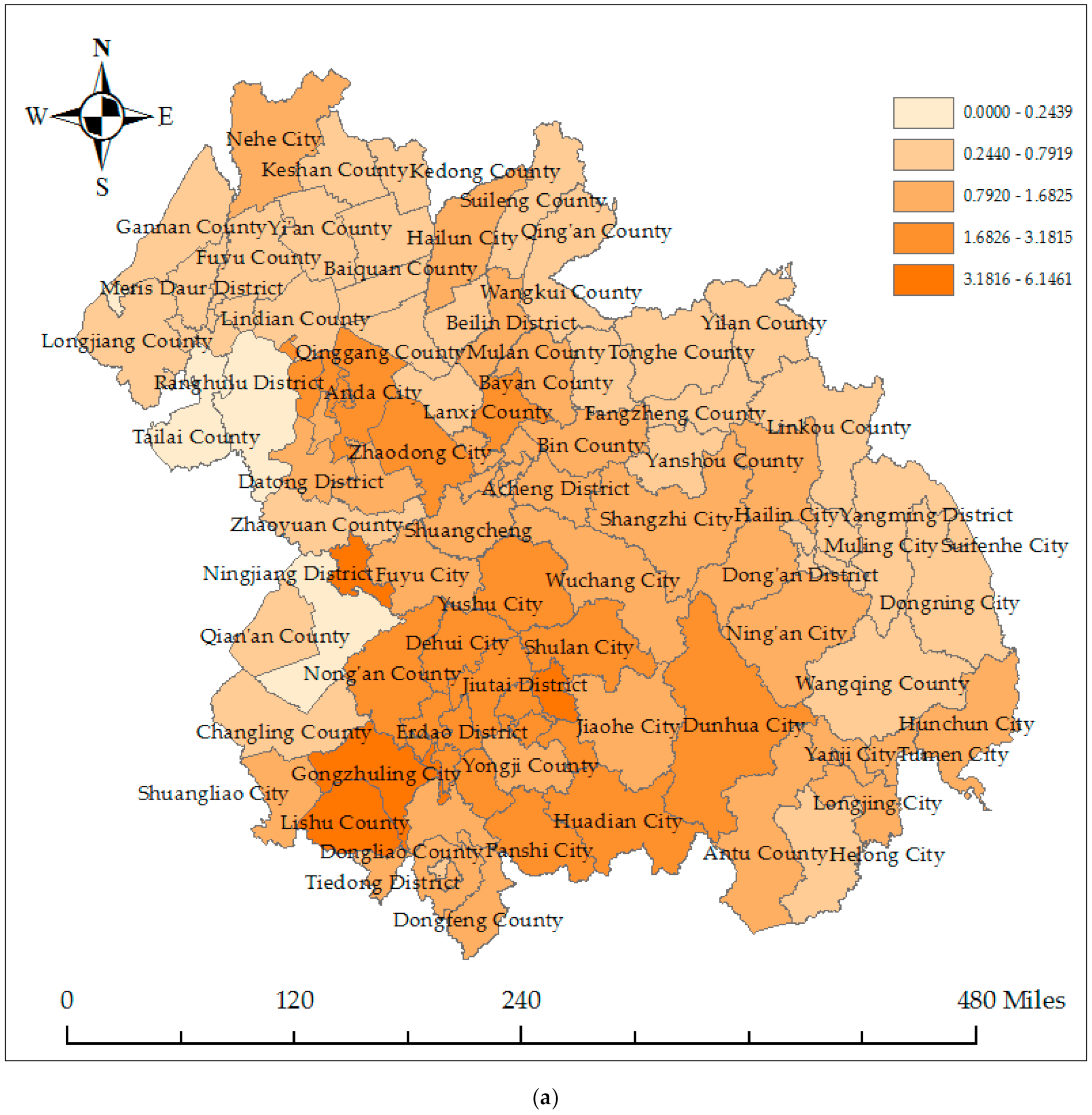
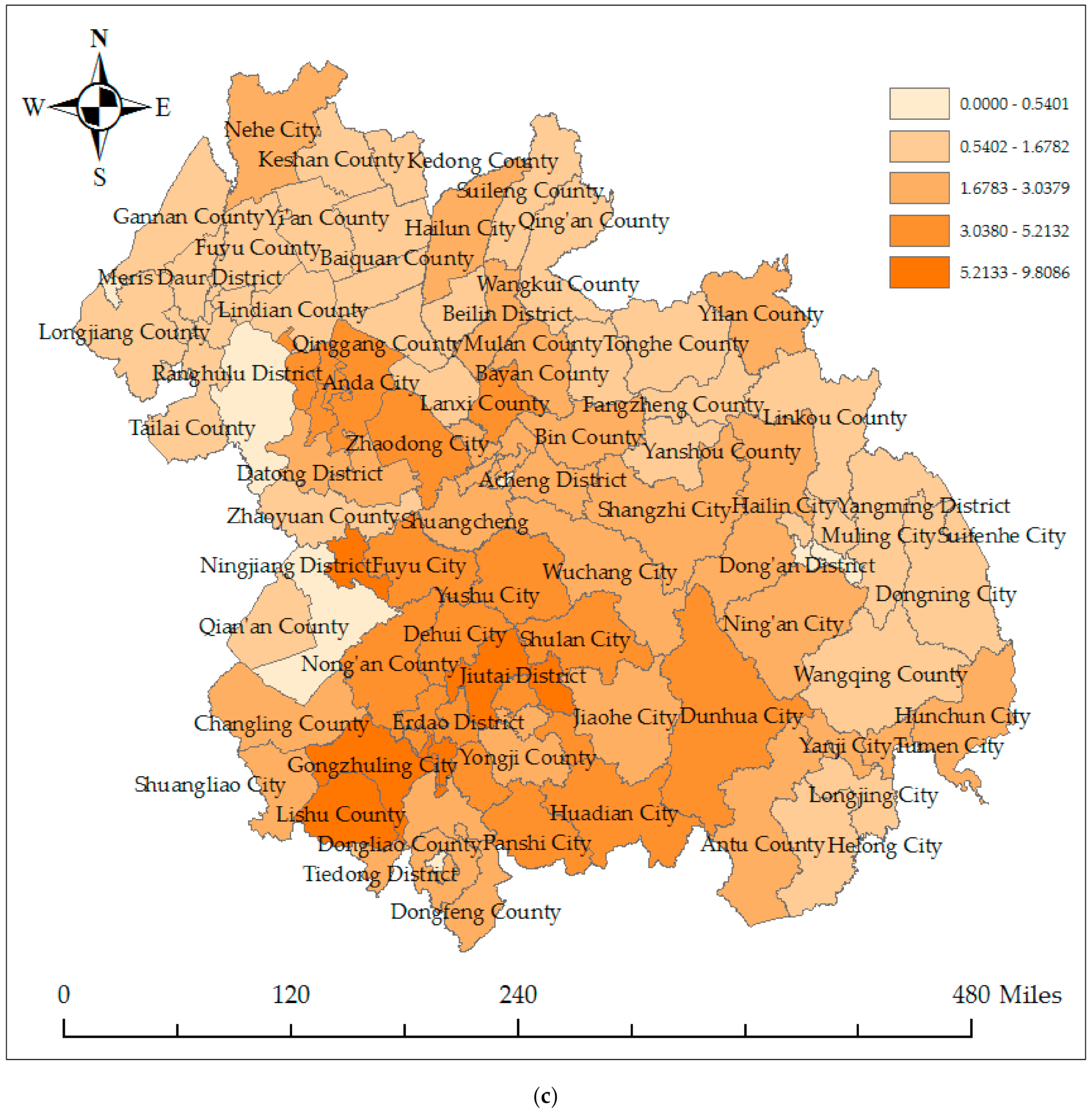
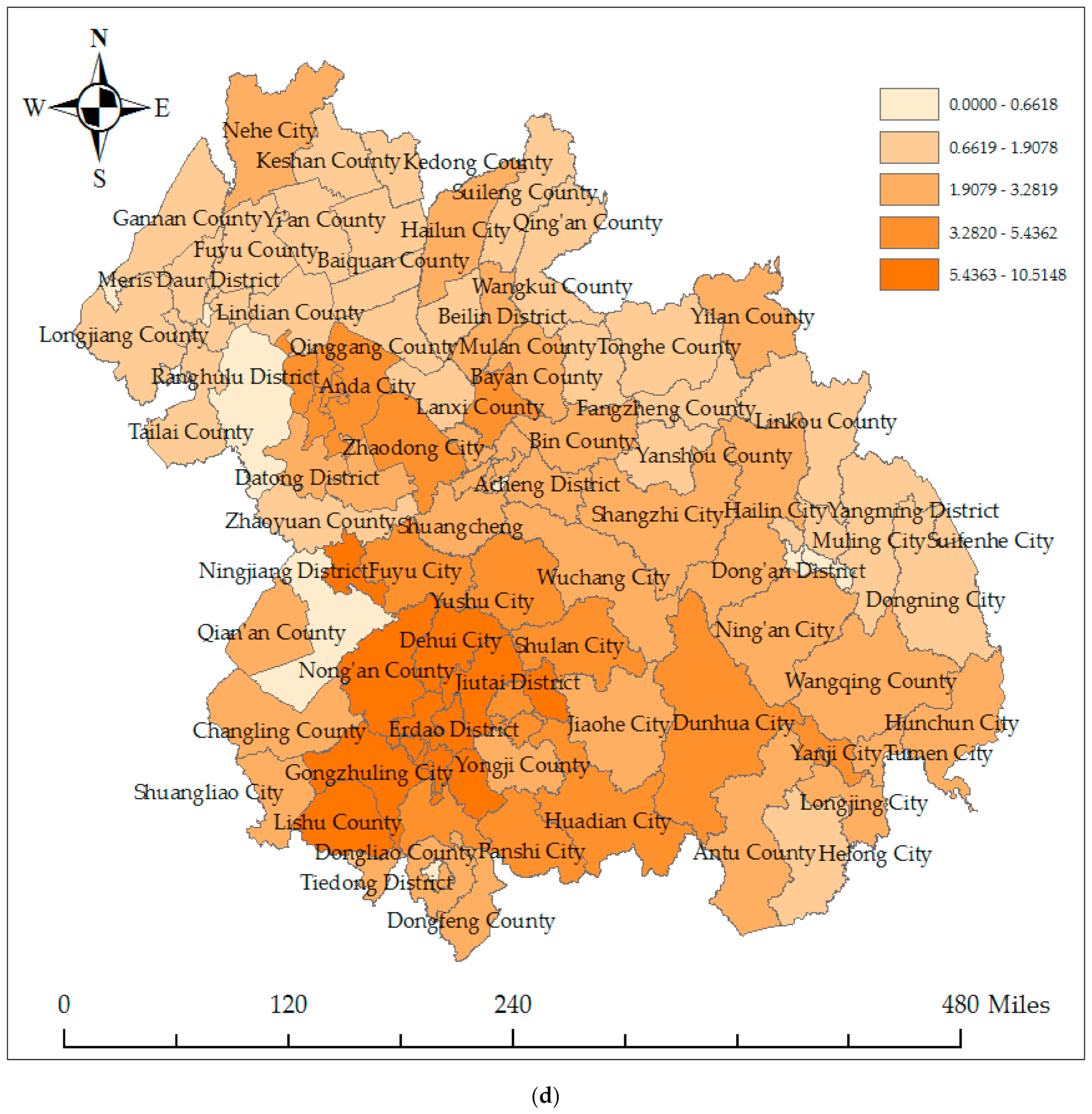
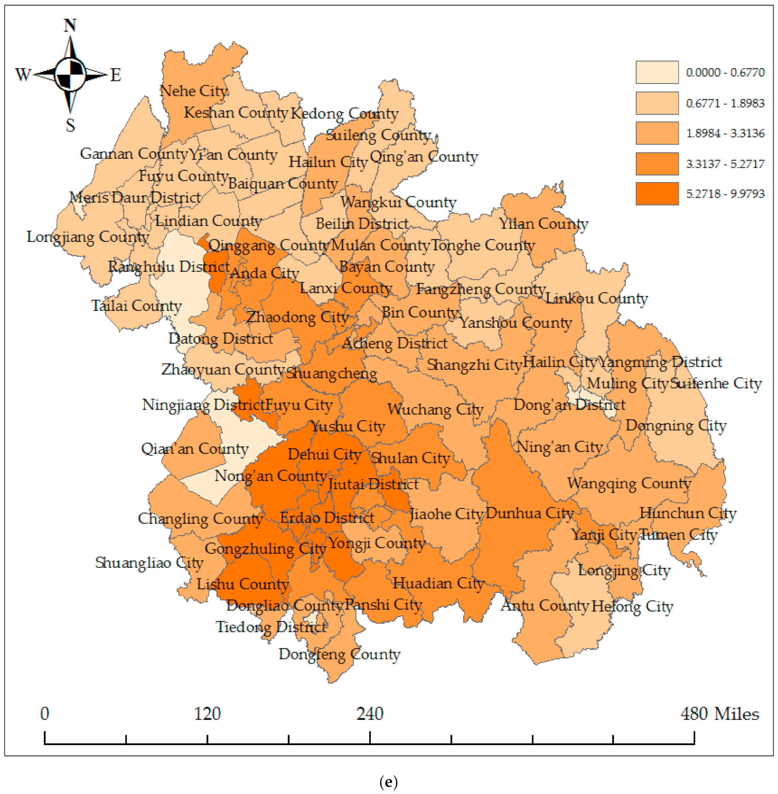
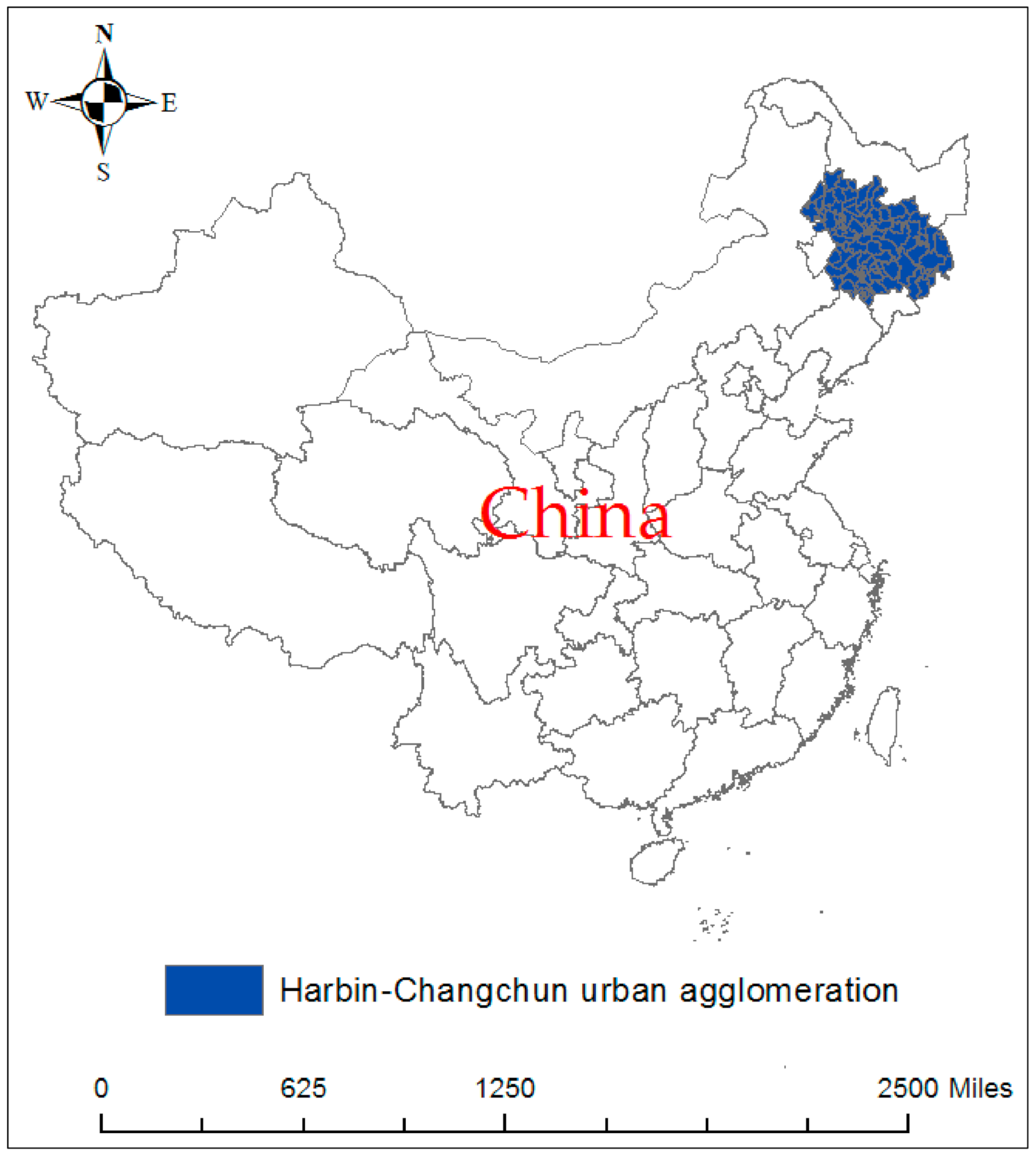
3.1. The Overall Distribution Characteristics and Patterns of County-Level Carbon Emissions in the Harbin–Changchun Urban Agglomeration
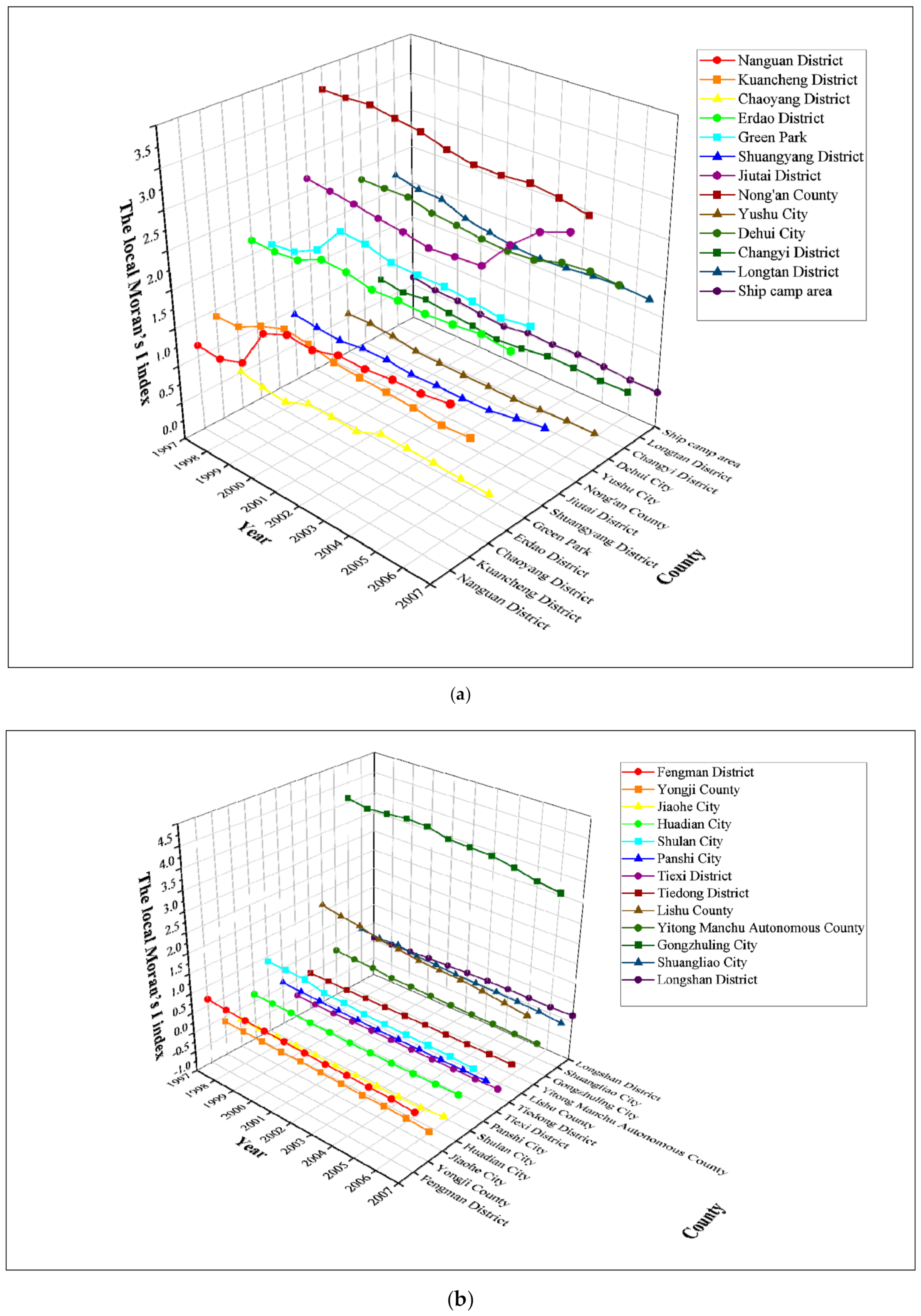
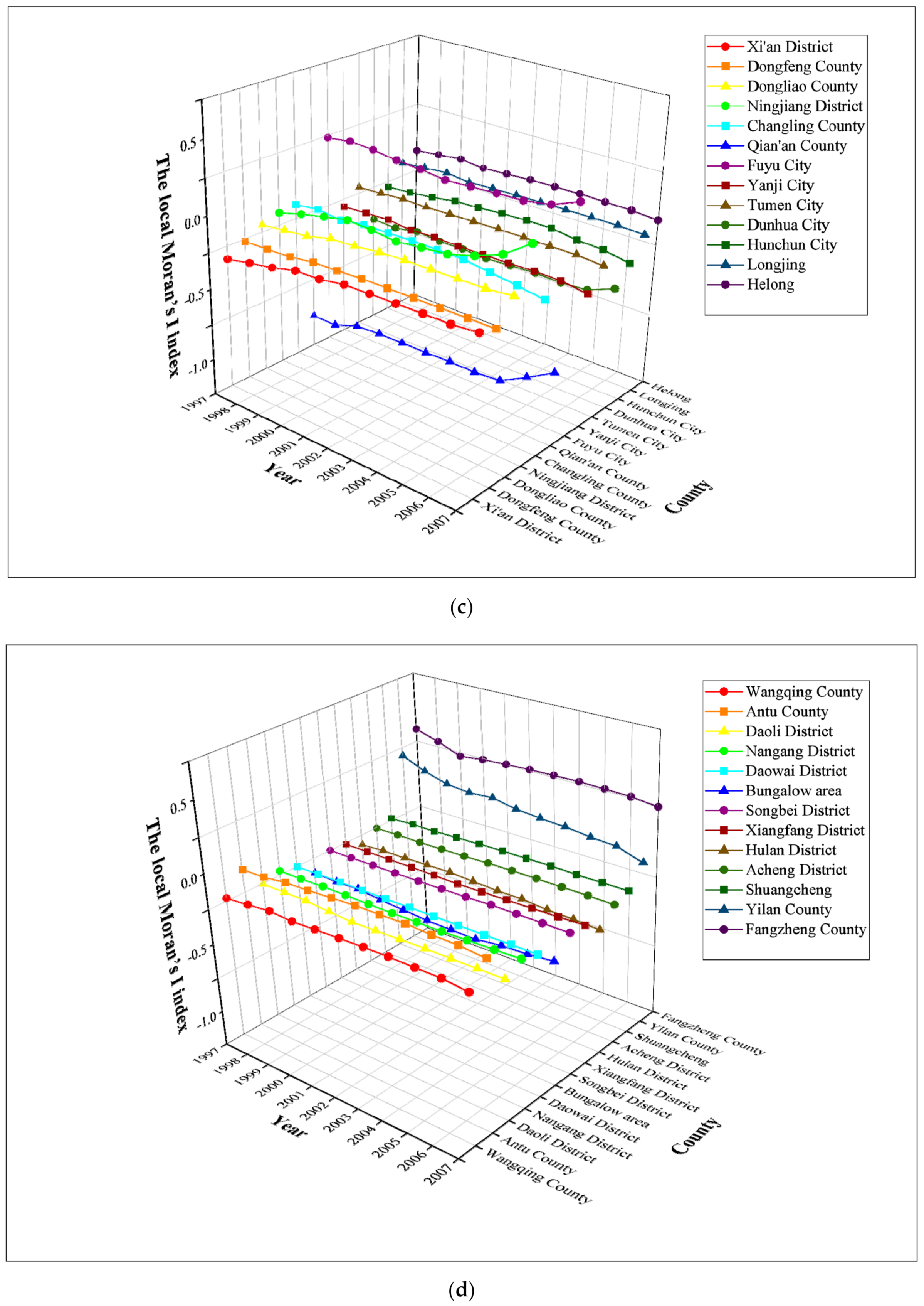
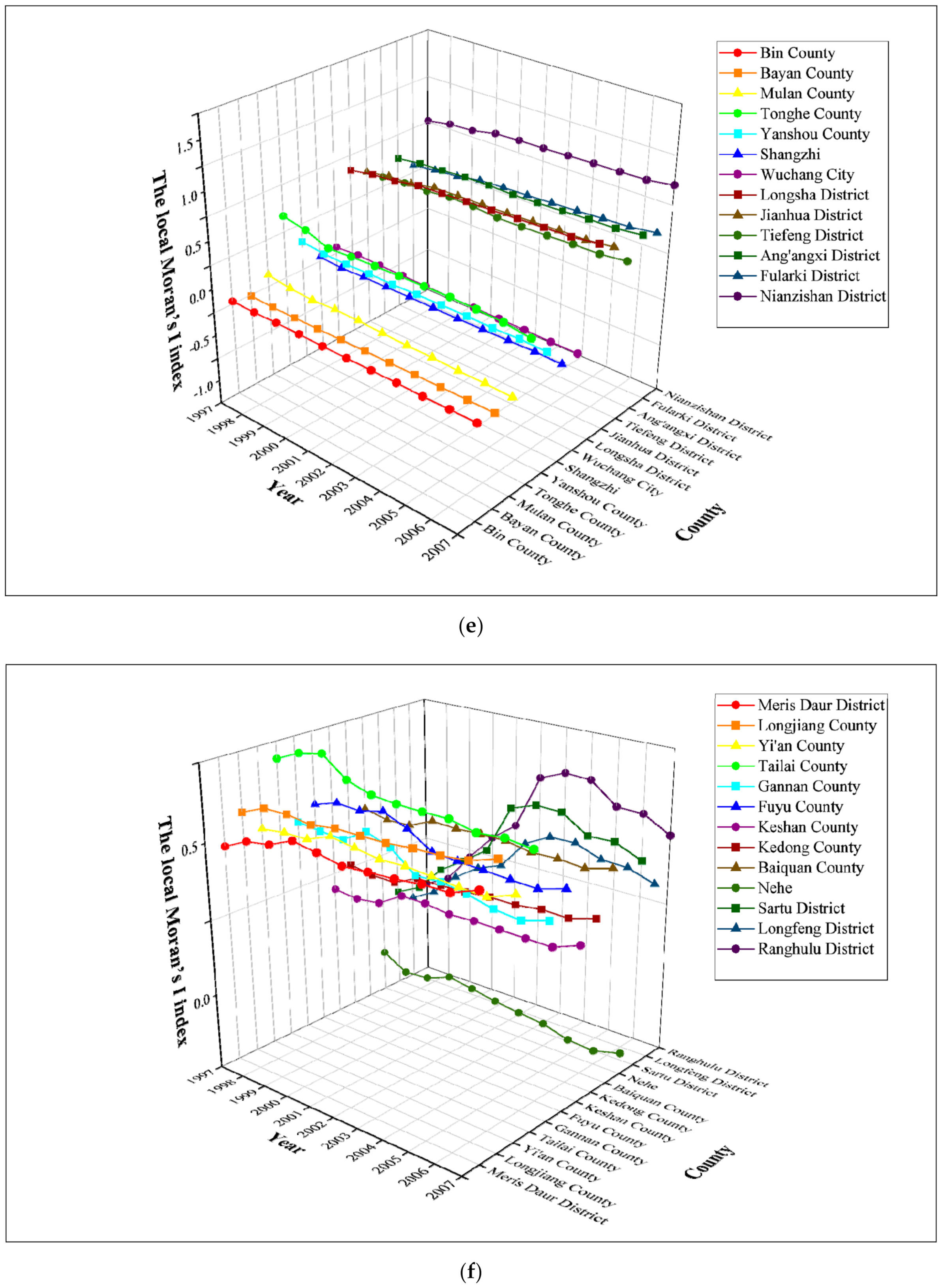
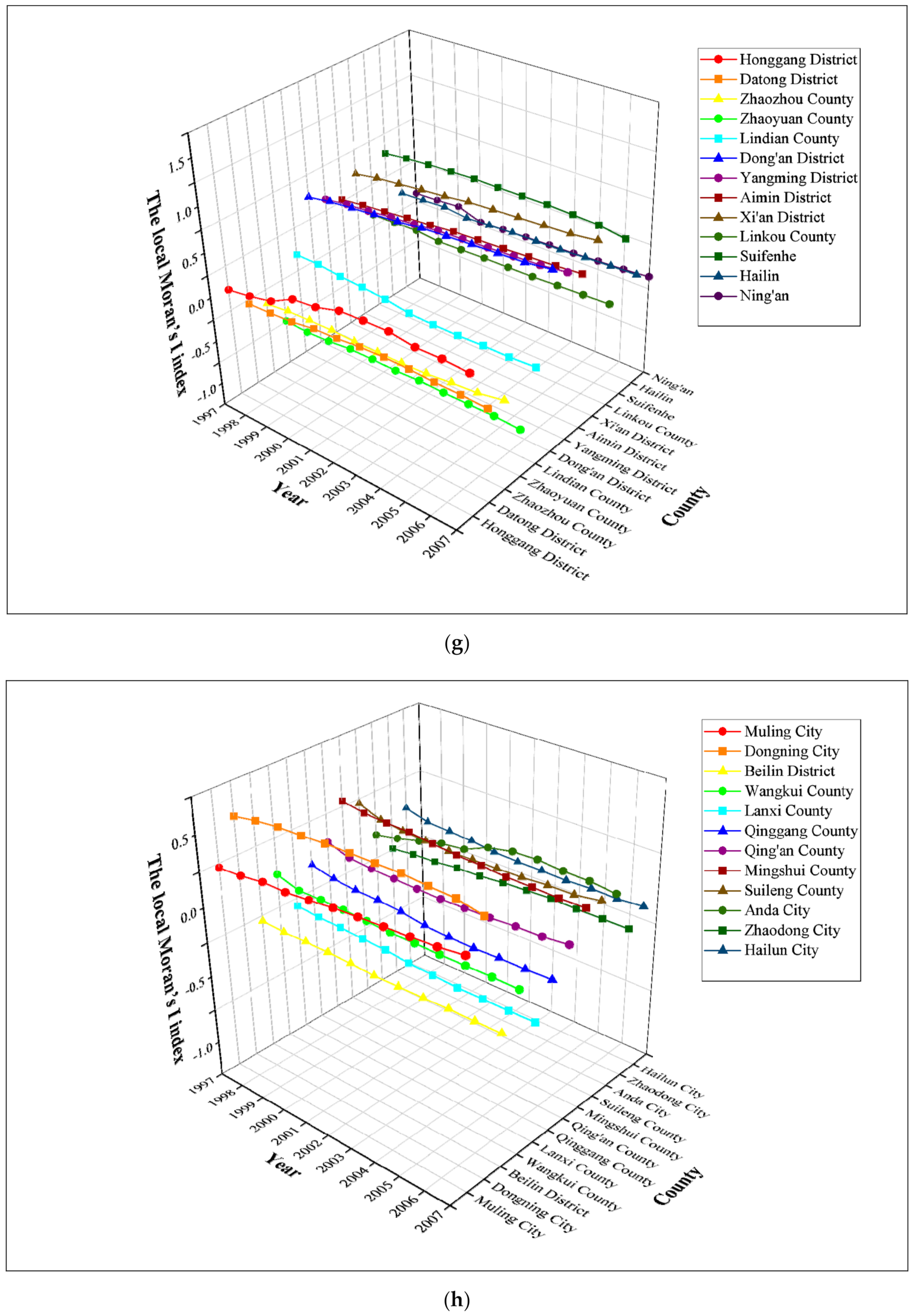
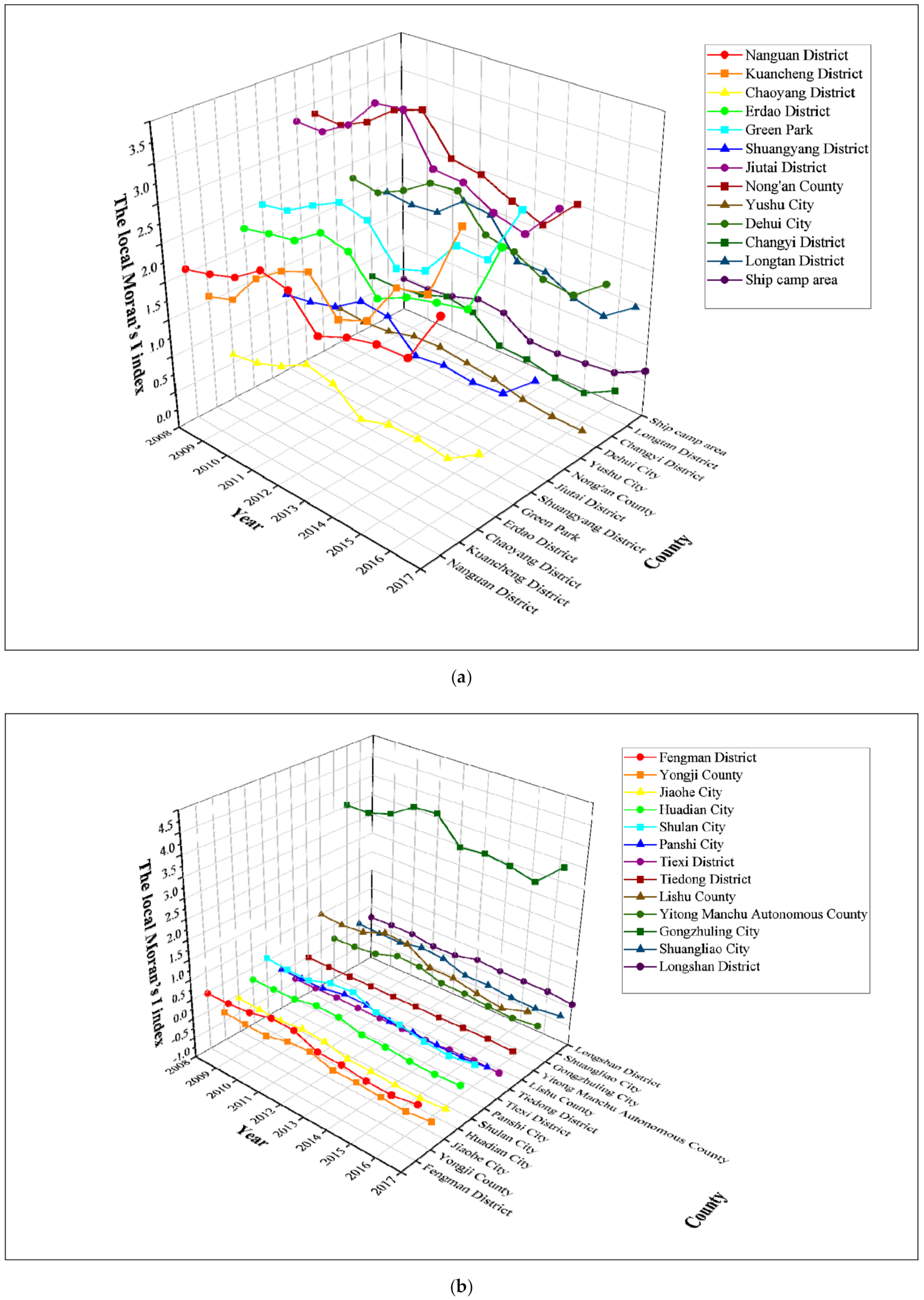
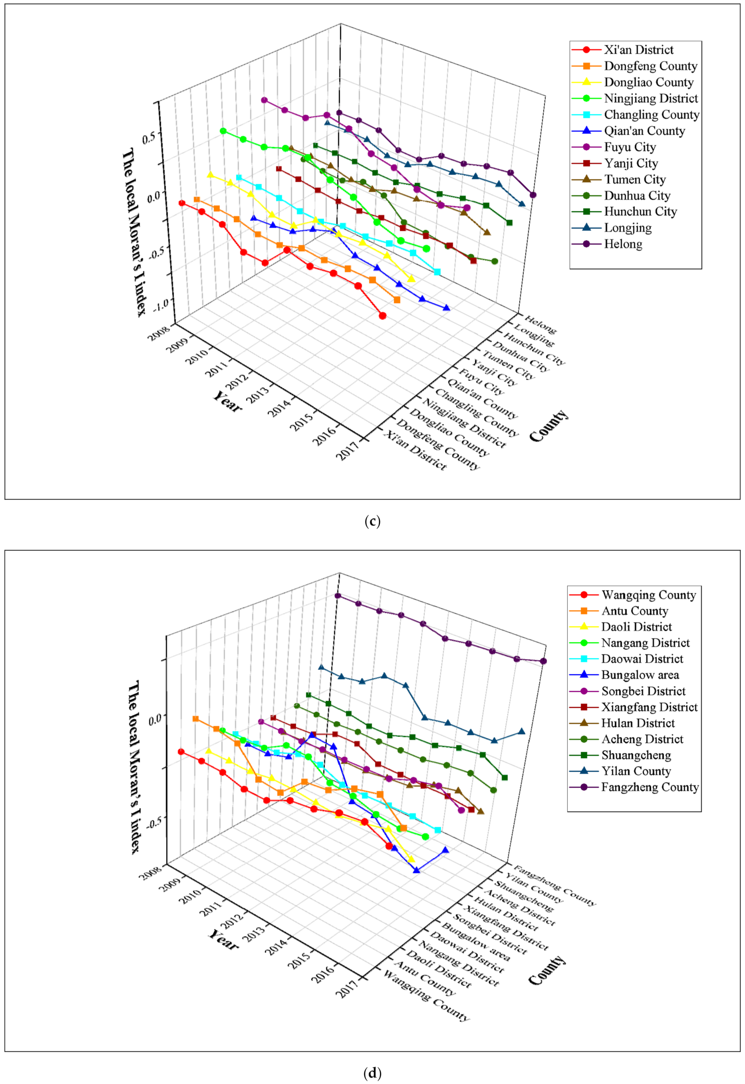
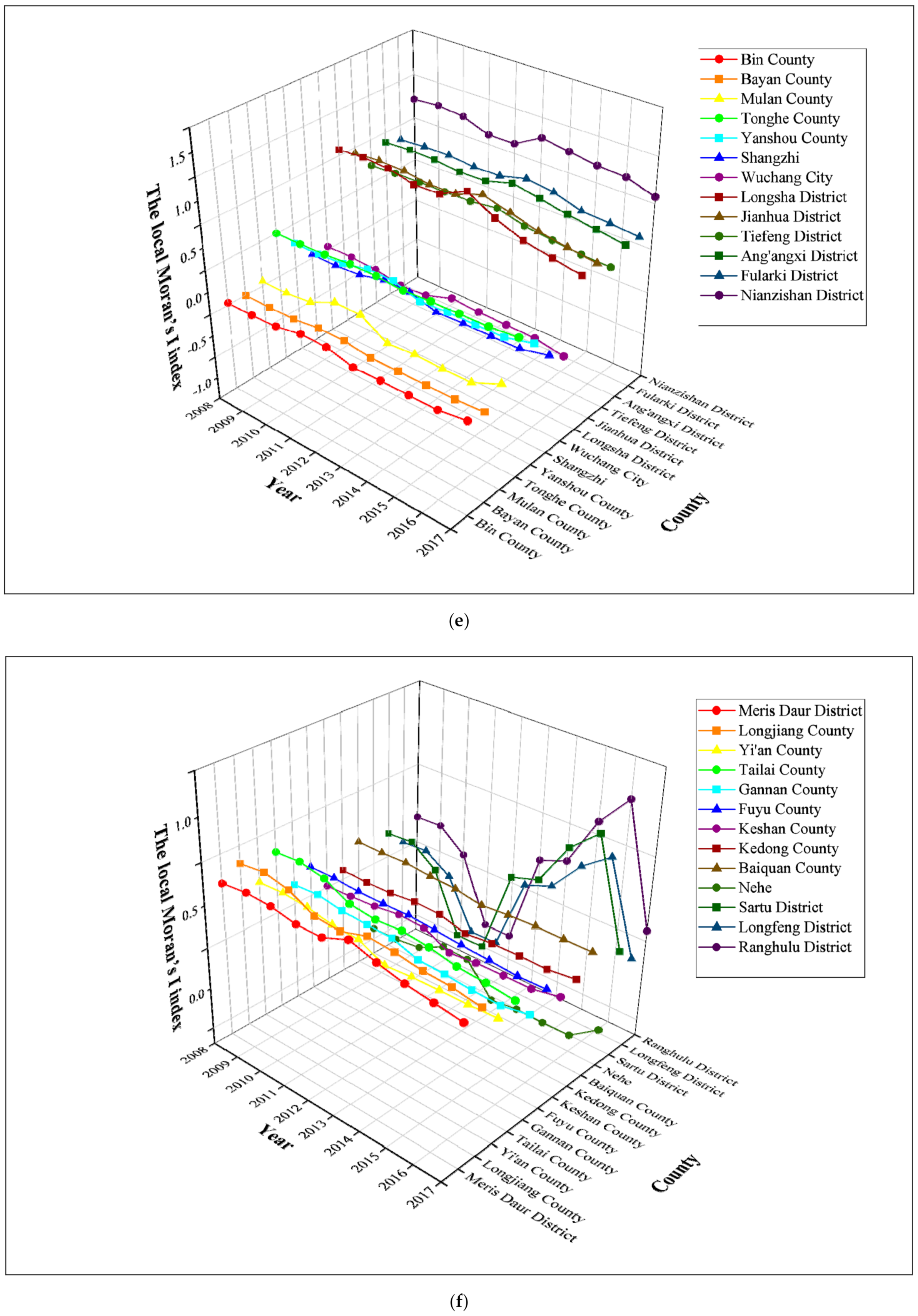
3.2. The Local Distribution Characteristics and Patterns of County-Level Carbon Emissions in the Harbin–Changchun Urban Agglomeration
4. Conclusions
Funding
Institutional Review Board Statement
Informed Consent Statement
Data Availability Statement
Conflicts of Interest
Appendix A. The Spatial Distribution of the Carbon Emissions in Harbin–Changchun Urban Agglomeration in 1997

Appendix B. Establish the Spatial Weight Matrix
Appendix C

| Year | The Global Moran’s I Indexes |
|---|---|
| 1997 | 0.4852 |
| 1998 | 0.4831 |
| 1999 | 0.4928 |
| 2000 | 0.5071 |
| 2001 | 0.5067 |
| 2002 | 0.5022 |
| 2003 | 0.5065 |
| 2004 | 0.5083 |
| 2005 | 0.5114 |
| 2006 | 0.5143 |
| 2007 | 0.5202 |
| 2008 | 0.5236 |
| 2009 | 0.5237 |
| 2010 | 0.5389 |
| 2011 | 0.5724 |
| 2012 | 0.5687 |
| 2013 | 0.5089 |
| 2014 | 0.5127 |
| 2015 | 0.5145 |
| 2016 | 0.5111 |
| 2017 | 0.5527 |
| 1997 | 1998 | 1999 | 2000 | 2001 | 2002 | 2003 | 2004 | 2005 | 2006 | 2007 | |
|---|---|---|---|---|---|---|---|---|---|---|---|
| Nanguan District | 1.1472 | 1.1229 | 1.2333 | 1.7679 | 1.9064 | 1.8735 | 1.9701 | 1.9629 | 1.9984 | 2.0023 | 2.0497 |
| Kuancheng District | 1.4101 | 1.4195 | 1.5842 | 1.7003 | 1.6623 | 1.5881 | 1.5579 | 1.5403 | 1.5182 | 1.4775 | 1.5026 |
| Chaoyang District | 0.5172 | 0.4594 | 0.4206 | 0.5652 | 0.5582 | 0.5418 | 0.6803 | 0.6722 | 0.6660 | 0.6462 | 0.6425 |
| Erdao District | 2.1768 | 2.1643 | 2.1903 | 2.3354 | 2.3161 | 2.2385 | 2.2513 | 2.2349 | 2.2592 | 2.2968 | 2.2516 |
| Green Park | 2.0109 | 2.0496 | 2.2101 | 2.5766 | 2.5501 | 2.4561 | 2.4430 | 2.4449 | 2.4114 | 2.3607 | 2.4119 |
| Shuangyang District | 0.9306 | 0.8921 | 0.8689 | 0.9104 | 0.9175 | 0.8793 | 0.8944 | 0.8898 | 0.9022 | 0.9671 | 1.0225 |
| Jiutai District | 2.6626 | 2.6197 | 2.5774 | 2.5189 | 2.4771 | 2.4075 | 2.4321 | 2.4606 | 2.8466 | 3.1332 | 3.2639 |
| Nong’an County | 3.7080 | 3.7104 | 3.7266 | 3.6664 | 3.6161 | 3.5145 | 3.4446 | 3.4404 | 3.4692 | 3.4202 | 3.3435 |
| Yushu City | 0.5579 | 0.5671 | 0.5345 | 0.4763 | 0.4652 | 0.4546 | 0.4565 | 0.4500 | 0.4720 | 0.4947 | 0.5030 |
| Dehui City | 2.3409 | 2.3463 | 2.3499 | 2.2625 | 2.2295 | 2.1819 | 2.1596 | 2.1812 | 2.2841 | 2.3136 | 2.2852 |
| Changyi District | 0.8172 | 0.7713 | 0.8110 | 0.7654 | 0.7325 | 0.6916 | 0.7200 | 0.7752 | 0.7729 | 0.7562 | 0.7698 |
| Longtan District | 2.1984 | 2.1211 | 2.1073 | 1.9698 | 1.9088 | 1.8486 | 1.8247 | 1.8385 | 1.8747 | 1.8845 | 1.8566 |
| Ship camp area | 0.6130 | 0.5577 | 0.5429 | 0.4922 | 0.4675 | 0.5202 | 0.5114 | 0.5260 | 0.5120 | 0.4893 | 0.4821 |
| Fengman District | 0.6664 | 0.6206 | 0.5963 | 0.5781 | 0.5614 | 0.5357 | 0.5189 | 0.5145 | 0.5070 | 0.4968 | 0.4572 |
| Yongji County | −0.1160 | −0.1421 | −0.1515 | −0.1732 | −0.1588 | −0.1747 | −0.1940 | −0.2047 | −0.2043 | −0.2178 | −0.2512 |
| Jiaohe City | −0.2824 | −0.2801 | −0.2455 | −0.2303 | −0.2239 | −0.2360 | −0.2263 | −0.2177 | −0.2188 | −0.2054 | −0.1340 |
| Huadian City | 0.1935 | 0.1788 | 0.1758 | 0.1567 | 0.1507 | 0.1380 | 0.1361 | 0.1341 | 0.1391 | 0.1430 | 0.1607 |
| Shulan City | 0.8738 | 0.8730 | 0.8456 | 0.7278 | 0.7046 | 0.6631 | 0.6393 | 0.6309 | 0.6224 | 0.6045 | 0.5644 |
| Panshi City | 0.1166 | 0.0956 | 0.0789 | 0.0526 | 0.0481 | 0.0381 | 0.0344 | 0.0316 | 0.0311 | 0.0346 | 0.0373 |
| Tiexi District | −0.4386 | −0.4552 | −0.4600 | −0.4335 | −0.4388 | −0.4412 | −0.4420 | −0.4427 | −0.4335 | −0.4269 | −0.4112 |
| Tiedong District | −0.0062 | −0.0116 | −0.0181 | −0.0168 | −0.0119 | −0.0107 | −0.0091 | −0.0090 | −0.0098 | −0.0110 | −0.0135 |
| Lishu County | 1.6621 | 1.5647 | 1.5013 | 1.3565 | 1.3159 | 1.2366 | 1.2132 | 1.1971 | 1.1363 | 1.0657 | 0.9989 |
| Yitong Manchu Autonomous County | 0.2486 | 0.2137 | 0.1929 | 0.1434 | 0.1368 | 0.1151 | 0.1046 | 0.0975 | 0.0887 | 0.0759 | 0.0797 |
| Gongzhuling City | 4.1096 | 4.0099 | 4.0441 | 4.0850 | 4.0603 | 3.9234 | 3.9010 | 3.8767 | 3.7765 | 3.6419 | 3.5585 |
| Shuangliao City | 0.4887 | 0.4313 | 0.4571 | 0.3640 | 0.3464 | 0.3046 | 0.2944 | 0.2868 | 0.2626 | 0.2343 | 0.1821 |
| Longshan District | 0.0604 | 0.0790 | 0.0963 | 0.1283 | 0.1372 | 0.1566 | 0.1632 | 0.1638 | 0.1624 | 0.1554 | 0.1681 |
| Xi’an District | −0.0904 | −0.0556 | −0.0259 | 0.0162 | 0.0223 | 0.0499 | 0.0548 | 0.0576 | 0.0610 | 0.0620 | 0.0788 |
| Dongfeng County | −0.0180 | −0.0116 | −0.0039 | 0.0202 | 0.0260 | 0.0348 | 0.0373 | 0.0384 | 0.0401 | 0.0417 | 0.0426 |
| Dongliao County | 0.0486 | 0.0689 | 0.0863 | 0.1288 | 0.1376 | 0.1581 | 0.1657 | 0.1673 | 0.1697 | 0.1729 | 0.1904 |
| Ningjiang District | 0.0867 | 0.1328 | 0.1716 | 0.2043 | 0.1954 | 0.1778 | 0.1968 | 0.2137 | 0.2635 | 0.3333 | 0.4601 |
| Changling County | 0.0989 | 0.1192 | 0.1009 | 0.1262 | 0.1272 | 0.1328 | 0.1319 | 0.1289 | 0.1068 | 0.0833 | 0.0558 |
| Qian’an County | −0.7776 | −0.7806 | −0.7201 | −0.7102 | −0.7081 | −0.7072 | −0.7027 | −0.7057 | −0.6914 | −0.5949 | −0.4891 |
| Fuyu City | 0.4841 | 0.5077 | 0.4971 | 0.4760 | 0.4672 | 0.4458 | 0.4545 | 0.4646 | 0.4717 | 0.5010 | 0.5745 |
| Yanji City | −0.0560 | −0.0452 | −0.0389 | −0.0573 | −0.0496 | −0.0542 | −0.0525 | −0.0518 | −0.0450 | −0.0484 | −0.0737 |
| Tumen City | 0.0426 | 0.0523 | 0.0632 | 0.0607 | 0.0669 | 0.0697 | 0.0738 | 0.0760 | 0.0750 | 0.0756 | 0.0614 |
| Dunhua City | −0.2454 | −0.2532 | −0.2244 | −0.2388 | −0.2355 | −0.2451 | −0.2353 | −0.2263 | −0.2325 | −0.2196 | −0.1471 |
| Hunchun City | −0.0431 | −0.0309 | −0.0146 | 0.0131 | 0.0210 | 0.0336 | 0.0400 | 0.0419 | 0.0166 | 0.0090 | −0.0255 |
| Longjing | 0.0946 | 0.1115 | 0.1244 | 0.1066 | 0.1141 | 0.1194 | 0.1223 | 0.1251 | 0.1270 | 0.1276 | 0.1214 |
| Helong | 0.1494 | 0.1673 | 0.1844 | 0.1674 | 0.1776 | 0.1869 | 0.1889 | 0.1922 | 0.1892 | 0.1853 | 0.1725 |
| Wangqing County | 0.0196 | 0.0335 | 0.0505 | 0.0400 | 0.0487 | 0.0536 | 0.0595 | 0.0622 | 0.0591 | 0.0589 | 0.0398 |
| Antu County | 0.1608 | 0.1637 | 0.1853 | 0.1898 | 0.1979 | 0.2073 | 0.2079 | 0.2117 | 0.2022 | 0.1999 | 0.1836 |
| Daoli District | −0.0043 | −0.0052 | −0.0055 | −0.0225 | −0.0340 | −0.0290 | −0.0260 | −0.0227 | −0.0229 | −0.0219 | −0.0228 |
| Nangang District | 0.0289 | 0.0289 | 0.0323 | 0.0289 | 0.0262 | 0.0246 | 0.0248 | 0.0243 | 0.0302 | 0.0321 | 0.0380 |
| Daowai District | −0.0007 | 0.0002 | 0.0000 | 0.0000 | −0.0001 | −0.0001 | −0.0005 | −0.0011 | −0.0023 | −0.0026 | −0.0028 |
| Bungalow area | −0.1092 | −0.1178 | −0.1120 | −0.1319 | −0.1452 | −0.1600 | −0.1626 | −0.1659 | −0.1447 | −0.1372 | −0.1193 |
| Songbei District | 0.0001 | 0.0002 | 0.0003 | 0.0001 | −0.0002 | 0.0020 | 0.0039 | 0.0092 | 0.0076 | 0.0066 | 0.0041 |
| Xiangfang District | −0.0129 | −0.0130 | −0.0155 | −0.0185 | −0.0209 | −0.0246 | −0.0229 | −0.0210 | −0.0181 | −0.0165 | −0.0124 |
| Hulan District | −0.0743 | −0.0652 | −0.0658 | −0.0624 | −0.0592 | −0.0691 | −0.0789 | −0.0783 | −0.0941 | −0.1006 | −0.1104 |
| Acheng District | −0.0050 | −0.0036 | −0.0070 | −0.0048 | −0.0013 | 0.0027 | 0.0042 | 0.0051 | 0.0027 | 0.0011 | −0.0023 |
| Shuangcheng | 0.0144 | 0.0202 | 0.0185 | 0.0254 | 0.0294 | 0.0320 | 0.0328 | 0.0347 | 0.0285 | 0.0296 | 0.0298 |
| Yilan County | 0.4380 | 0.3679 | 0.3187 | 0.3024 | 0.3130 | 0.2806 | 0.2647 | 0.2546 | 0.2343 | 0.2237 | 0.1637 |
| Fangzheng County | 0.5903 | 0.5382 | 0.4732 | 0.4924 | 0.5020 | 0.5102 | 0.5151 | 0.5170 | 0.5132 | 0.5084 | 0.4879 |
| Bin County | 0.0272 | 0.0242 | 0.0279 | 0.0267 | 0.0196 | 0.0206 | 0.0190 | 0.0196 | 0.0115 | 0.0142 | 0.0149 |
| Bayan County | −0.0094 | −0.0206 | −0.0205 | −0.0183 | −0.0161 | −0.0128 | −0.0106 | −0.0089 | −0.0057 | −0.0046 | −0.0055 |
| Mulan County | 0.1252 | 0.0877 | 0.0732 | 0.0859 | 0.0834 | 0.0706 | 0.0602 | 0.0605 | 0.0480 | 0.0490 | 0.0387 |
| Tonghe County | 0.6691 | 0.6217 | 0.5304 | 0.5469 | 0.5578 | 0.5639 | 0.5686 | 0.5728 | 0.5647 | 0.5506 | 0.5127 |
| Yanshou County | 0.3055 | 0.2758 | 0.2687 | 0.2751 | 0.2709 | 0.2775 | 0.2795 | 0.2815 | 0.2741 | 0.2835 | 0.2744 |
| Shangzhi | 0.0450 | 0.0288 | 0.0360 | 0.0357 | 0.0391 | 0.0362 | 0.0357 | 0.0378 | 0.0407 | 0.0483 | 0.0397 |
| Wuchang City | 0.0639 | 0.0828 | 0.0733 | 0.0666 | 0.0623 | 0.0561 | 0.0550 | 0.0520 | 0.0497 | 0.0441 | 0.0426 |
| Longsha District | 0.8353 | 0.8814 | 0.9013 | 0.9498 | 0.9599 | 0.9716 | 0.9822 | 0.9937 | 1.0053 | 1.0144 | 1.0503 |
| Jianhua District | 0.7399 | 0.7821 | 0.7943 | 0.8460 | 0.8545 | 0.8569 | 0.8664 | 0.8769 | 0.8893 | 0.8957 | 0.9271 |
| Tiefeng District | 0.6035 | 0.6318 | 0.6351 | 0.6614 | 0.6578 | 0.6353 | 0.6380 | 0.6470 | 0.6590 | 0.6625 | 0.6943 |
| Ang’angxi District | 0.7344 | 0.7696 | 0.7815 | 0.8006 | 0.8047 | 0.7994 | 0.8070 | 0.8180 | 0.8316 | 0.8375 | 0.8681 |
| Fularki District | 0.5800 | 0.6172 | 0.6388 | 0.6851 | 0.7009 | 0.7113 | 0.7233 | 0.7362 | 0.7541 | 0.7666 | 0.8041 |
| Nianzishan District | 1.0104 | 1.0550 | 1.0687 | 1.1210 | 1.1321 | 1.1361 | 1.1452 | 1.1544 | 1.1585 | 1.1665 | 1.2049 |
| Meris Daur District | 0.7199 | 0.7575 | 0.7694 | 0.8035 | 0.7895 | 0.7720 | 0.7776 | 0.7815 | 0.7899 | 0.7902 | 0.8216 |
| Longjiang County | 0.8093 | 0.8425 | 0.8434 | 0.8316 | 0.8426 | 0.8416 | 0.8417 | 0.8489 | 0.8500 | 0.8584 | 0.8861 |
| Yi’an County | 0.7358 | 0.7453 | 0.7452 | 0.7759 | 0.7625 | 0.7493 | 0.7515 | 0.7441 | 0.7357 | 0.7311 | 0.7629 |
| Tailai County | 0.9439 | 0.9792 | 0.9952 | 0.9321 | 0.9054 | 0.8973 | 0.8943 | 0.8939 | 0.8744 | 0.8808 | 0.8702 |
| Gannan County | 0.7187 | 0.7093 | 0.7034 | 0.7501 | 0.7213 | 0.6550 | 0.6586 | 0.6455 | 0.6235 | 0.6141 | 0.6388 |
| Fuyu County | 0.7581 | 0.7828 | 0.7772 | 0.7956 | 0.7613 | 0.7084 | 0.7015 | 0.6967 | 0.6910 | 0.6866 | 0.7111 |
| Keshan County | 0.4438 | 0.4344 | 0.4445 | 0.4935 | 0.4934 | 0.4819 | 0.4854 | 0.4834 | 0.4816 | 0.4801 | 0.5133 |
| Kedong County | 0.5081 | 0.4946 | 0.4927 | 0.5313 | 0.5304 | 0.5341 | 0.5410 | 0.5401 | 0.5508 | 0.5475 | 0.5727 |
| Baiquan County | 0.6860 | 0.6675 | 0.6696 | 0.7049 | 0.7006 | 0.7045 | 0.7041 | 0.6884 | 0.6910 | 0.6829 | 0.7062 |
| Nehe | 0.1360 | 0.0895 | 0.0966 | 0.1285 | 0.1145 | 0.0984 | 0.0869 | 0.0784 | 0.0529 | 0.0465 | 0.0710 |
| Sartu District | 0.3422 | 0.3827 | 0.4710 | 0.5252 | 0.5857 | 0.7500 | 0.7805 | 0.7779 | 0.7219 | 0.7244 | 0.6863 |
| Longfeng District | 0.2975 | 0.3430 | 0.4223 | 0.4788 | 0.5112 | 0.6104 | 0.6546 | 0.6562 | 0.6236 | 0.6196 | 0.5894 |
| Ranghulu District | 0.3275 | 0.3717 | 0.4741 | 0.5659 | 0.6306 | 0.8148 | 0.8499 | 0.8455 | 0.7771 | 0.7745 | 0.7254 |
| Honggang District | 0.2309 | 0.2737 | 0.3335 | 0.4735 | 0.5041 | 0.5843 | 0.6012 | 0.6094 | 0.5696 | 0.5775 | 0.5616 |
| Datong District | −0.0478 | −0.0365 | −0.0186 | 0.0234 | 0.0372 | 0.0684 | 0.0825 | 0.0811 | 0.0681 | 0.0684 | 0.0558 |
| Zhaozhou County | −0.1668 | −0.1356 | −0.1234 | −0.1168 | −0.1224 | −0.1189 | −0.1138 | −0.1015 | −0.0704 | −0.0474 | 0.0077 |
| Zhaoyuan County | −0.4936 | −0.5085 | −0.4942 | −0.4610 | −0.4561 | −0.4610 | −0.4455 | −0.4499 | −0.4466 | −0.4426 | −0.4564 |
| Lindian County | 0.1860 | 0.1833 | 0.1531 | 0.1413 | 0.1209 | 0.0778 | 0.0701 | 0.0711 | 0.0824 | 0.0836 | 0.1009 |
| Dong’an District | 0.7520 | 0.7967 | 0.8245 | 0.8505 | 0.8737 | 0.9084 | 0.9246 | 0.9398 | 0.9549 | 0.9704 | 1.0074 |
| Yangming District | 0.6260 | 0.6646 | 0.6894 | 0.7202 | 0.7410 | 0.7713 | 0.7854 | 0.7989 | 0.8151 | 0.8301 | 0.8652 |
| Aimin District | 0.5224 | 0.5567 | 0.5802 | 0.6076 | 0.6285 | 0.6560 | 0.6693 | 0.6814 | 0.6980 | 0.7113 | 0.7359 |
| Xi’an District | 0.7241 | 0.7686 | 0.7956 | 0.8246 | 0.8479 | 0.8822 | 0.8980 | 0.9127 | 0.9270 | 0.9417 | 0.9762 |
| Linkou County | 0.1326 | 0.1372 | 0.1488 | 0.1198 | 0.1280 | 0.1368 | 0.1394 | 0.1419 | 0.1544 | 0.1638 | 0.1746 |
| Suifenhe | 0.7718 | 0.8018 | 0.8239 | 0.8350 | 0.8485 | 0.8450 | 0.8463 | 0.8492 | 0.8376 | 0.8256 | 0.7785 |
| Hailin | 0.1979 | 0.2084 | 0.2246 | 0.1920 | 0.2062 | 0.2201 | 0.2252 | 0.2303 | 0.2493 | 0.2616 | 0.2738 |
| Ning’an | 0.0972 | 0.1080 | 0.1283 | 0.0367 | 0.0481 | 0.0615 | 0.0722 | 0.0808 | 0.0971 | 0.1114 | 0.1373 |
| Muling City | 0.4701 | 0.4813 | 0.5063 | 0.5064 | 0.5241 | 0.5441 | 0.5565 | 0.5675 | 0.5772 | 0.5896 | 0.6139 |
| Dongning City | 0.7629 | 0.7939 | 0.8131 | 0.8197 | 0.8309 | 0.8347 | 0.8357 | 0.8398 | 0.8285 | 0.8226 | 0.7857 |
| Beilin District | −0.0397 | −0.0482 | −0.0454 | −0.0449 | −0.0484 | −0.0581 | −0.0540 | −0.0509 | −0.0442 | −0.0440 | −0.0411 |
| Wangkui County | 0.2384 | 0.1891 | 0.1925 | 0.1923 | 0.1849 | 0.1768 | 0.1776 | 0.1760 | 0.1790 | 0.1809 | 0.1784 |
| Lanxi County | −0.0585 | −0.0710 | −0.0743 | −0.0846 | −0.0908 | −0.1093 | −0.1187 | −0.1275 | −0.1259 | −0.1252 | −0.1208 |
| Qinggang County | 0.1857 | 0.1490 | 0.1330 | 0.1317 | 0.1193 | 0.0924 | 0.0837 | 0.0806 | 0.0883 | 0.0891 | 0.0961 |
| Qing’an County | 0.2940 | 0.2415 | 0.2277 | 0.2227 | 0.2182 | 0.2154 | 0.2211 | 0.2263 | 0.2395 | 0.2430 | 0.2628 |
| Mingshui County | 0.5393 | 0.5108 | 0.5009 | 0.4974 | 0.4777 | 0.4618 | 0.4566 | 0.4433 | 0.4425 | 0.4377 | 0.4420 |
| Suileng County | 0.4650 | 0.4051 | 0.3845 | 0.3764 | 0.3666 | 0.3695 | 0.3745 | 0.3789 | 0.3933 | 0.3963 | 0.4244 |
| Anda City | 0.1750 | 0.2097 | 0.2546 | 0.2992 | 0.3203 | 0.3965 | 0.4329 | 0.4409 | 0.4277 | 0.4261 | 0.4075 |
| Zhaodong City | 0.0103 | 0.0296 | 0.0371 | 0.0577 | 0.0630 | 0.0811 | 0.0915 | 0.1012 | 0.0974 | 0.0990 | 0.0994 |
| Hailun City | 0.2666 | 0.2200 | 0.2107 | 0.2011 | 0.1810 | 0.1750 | 0.1743 | 0.1703 | 0.1796 | 0.1758 | 0.1919 |
| 2008 | 2009 | 2010 | 2011 | 2012 | 2013 | 2014 | 2015 | 2016 | 2017 | |
|---|---|---|---|---|---|---|---|---|---|---|
| Nanguan District | 2.0534 | 2.1459 | 2.2621 | 2.5088 | 2.4225 | 2.0186 | 2.1763 | 2.2697 | 2.2862 | 2.9442 |
| Kuancheng District | 1.5671 | 1.6855 | 2.1242 | 2.3795 | 2.5288 | 2.0948 | 2.2516 | 2.8109 | 2.8981 | 3.8136 |
| Chaoyang District | 0.6229 | 0.6798 | 0.8125 | 1.0219 | 0.9455 | 0.6462 | 0.7722 | 0.7828 | 0.7314 | 0.9955 |
| Erdao District | 2.2452 | 2.3231 | 2.3827 | 2.6291 | 2.5453 | 2.1079 | 2.2886 | 2.3878 | 2.4711 | 3.3565 |
| Green Park | 2.4558 | 2.5175 | 2.7235 | 2.9061 | 2.8244 | 2.3677 | 2.4941 | 2.9599 | 2.9399 | 3.6616 |
| Shuangyang District | 1.0957 | 1.1530 | 1.2484 | 1.4911 | 1.4483 | 1.0870 | 1.1369 | 1.0968 | 1.1356 | 1.4871 |
| Jiutai District | 3.3477 | 3.3334 | 3.5439 | 3.9332 | 3.9719 | 3.3809 | 3.3515 | 3.1254 | 3.0152 | 3.4565 |
| Nong’an County | 3.3543 | 3.3263 | 3.4882 | 3.7594 | 3.8796 | 3.4048 | 3.3435 | 3.1599 | 3.0129 | 3.4014 |
| Yushu City | 0.5081 | 0.4796 | 0.5055 | 0.6062 | 0.6256 | 0.5731 | 0.5291 | 0.4283 | 0.3843 | 0.3827 |
| Dehui City | 2.2871 | 2.2236 | 2.3912 | 2.6224 | 2.6621 | 2.2185 | 2.1481 | 1.9383 | 1.8899 | 2.1927 |
| Changyi District | 0.7520 | 0.7388 | 0.7981 | 0.9338 | 0.8649 | 0.5537 | 0.5354 | 0.4544 | 0.4197 | 0.6427 |
| Longtan District | 1.8821 | 1.8361 | 1.8707 | 2.1707 | 2.1225 | 1.6213 | 1.6361 | 1.4386 | 1.3563 | 1.6459 |
| Ship camp area | 0.4669 | 0.4658 | 0.5212 | 0.6438 | 0.6017 | 0.3484 | 0.3475 | 0.3802 | 0.4300 | 0.6355 |
| Fengman District | 0.4538 | 0.4728 | 0.5213 | 0.6654 | 0.6450 | 0.4066 | 0.3954 | 0.3118 | 0.2898 | 0.3904 |
| Yongji County | −0.2631 | −0.2918 | −0.3083 | −0.1603 | −0.1213 | −0.2918 | −0.2903 | −0.3408 | −0.3695 | −0.2853 |
| Jiaohe City | −0.0990 | −0.1252 | −0.1347 | −0.0620 | −0.0976 | −0.2386 | −0.2508 | −0.2841 | −0.2965 | −0.2398 |
| Huadian City | 0.1918 | 0.2048 | 0.2150 | 0.3284 | 0.3090 | 0.1509 | 0.1331 | 0.0759 | 0.0550 | 0.1004 |
| Shulan City | 0.5635 | 0.5178 | 0.5008 | 0.6976 | 0.7335 | 0.5062 | 0.4696 | 0.3465 | 0.2889 | 0.3696 |
| Panshi City | 0.0544 | 0.0587 | 0.0734 | 0.1887 | 0.1909 | 0.0406 | 0.0423 | 0.0049 | 0.0005 | 0.0578 |
| Tiexi District | −0.4128 | −0.4004 | −0.3803 | −0.3916 | −0.3809 | −0.3817 | −0.3855 | −0.3439 | −0.3185 | −0.3300 |
| Tiedong District | −0.0132 | −0.0133 | −0.0177 | −0.0123 | −0.0175 | −0.0114 | −0.0110 | 0.0043 | 0.0136 | −0.0132 |
| Lishu County | 0.9812 | 0.9385 | 0.9872 | 1.2104 | 1.1682 | 0.8092 | 0.7998 | 0.6725 | 0.5812 | 0.7732 |
| Yitong Manchu Autonomous County | 0.1223 | 0.1467 | 0.2061 | 0.3984 | 0.3755 | 0.1982 | 0.1864 | 0.1288 | 0.1032 | 0.1864 |
| Gongzhuling City | 3.5228 | 3.5171 | 3.6880 | 4.0480 | 4.0831 | 3.4750 | 3.5325 | 3.4528 | 3.2950 | 3.8554 |
| Shuangliao City | 0.1669 | 0.1339 | 0.1297 | 0.2418 | 0.1912 | −0.0105 | −0.0072 | −0.0734 | −0.0883 | 0.0004 |
| Longshan District | 0.1692 | 0.1837 | 0.1739 | 0.0846 | 0.0866 | 0.2188 | 0.1641 | 0.1610 | 0.1585 | 0.0845 |
| Xi’an District | 0.0748 | 0.0900 | 0.0707 | −0.0791 | −0.0717 | 0.1415 | 0.1043 | 0.1496 | 0.1493 | 0.0089 |
| Dongfeng County | 0.0380 | 0.0491 | 0.0467 | 0.0057 | 0.0084 | 0.0820 | 0.0786 | 0.1089 | 0.1192 | 0.0592 |
| Dongliao County | 0.1942 | 0.2102 | 0.1984 | 0.1035 | 0.1028 | 0.2455 | 0.2223 | 0.2497 | 0.2402 | 0.1480 |
| Ningjiang District | 0.5236 | 0.5319 | 0.5472 | 0.6191 | 0.6251 | 0.5260 | 0.4704 | 0.3524 | 0.2935 | 0.3273 |
| Changling County | 0.0414 | 0.0418 | 0.0319 | −0.0003 | −0.0018 | 0.0548 | 0.0578 | 0.0970 | 0.1149 | 0.0526 |
| Qian’an County | −0.4226 | −0.3973 | −0.3620 | −0.2434 | −0.1657 | −0.2943 | −0.3077 | −0.3538 | −0.3827 | −0.3553 |
| Fuyu City | 0.6217 | 0.6094 | 0.6184 | 0.7207 | 0.6831 | 0.5539 | 0.5196 | 0.4224 | 0.3756 | 0.4470 |
| Yanji City | −0.0724 | −0.0834 | −0.1020 | −0.1174 | −0.1172 | −0.0865 | −0.0849 | −0.0600 | −0.0486 | −0.0854 |
| Tumen City | 0.0602 | 0.0663 | 0.0618 | 0.0161 | 0.0173 | 0.0935 | 0.1080 | 0.1540 | 0.1692 | 0.0873 |
| Dunhua City | −0.1072 | −0.1348 | −0.1411 | −0.0656 | −0.1061 | −0.2733 | −0.2784 | −0.3036 | −0.3081 | −0.2451 |
| Hunchun City | −0.0339 | −0.0248 | −0.0235 | −0.0440 | −0.0462 | 0.0092 | 0.0215 | 0.0700 | 0.0959 | 0.0332 |
| Longjing | 0.1222 | 0.1313 | 0.1231 | 0.0521 | 0.0527 | 0.1422 | 0.1543 | 0.2017 | 0.2190 | 0.1278 |
| Helong | 0.1667 | 0.1716 | 0.1546 | 0.0452 | 0.0400 | 0.1579 | 0.1702 | 0.2328 | 0.2602 | 0.1480 |
| Wangqing County | 0.0405 | 0.0451 | 0.0418 | 0.0127 | 0.0128 | 0.0665 | 0.0815 | 0.1192 | 0.1345 | 0.0824 |
| Antu County | 0.1690 | 0.1671 | 0.1470 | 0.0245 | 0.0140 | 0.1180 | 0.1318 | 0.1919 | 0.2204 | 0.1237 |
| Daoli District | −0.0245 | −0.0225 | −0.0249 | −0.0066 | −0.0085 | −0.0195 | −0.0257 | −0.0055 | 0.0201 | −0.0631 |
| Nangang District | 0.0483 | 0.0488 | 0.0593 | 0.1215 | 0.1166 | 0.0416 | 0.0313 | −0.0026 | −0.0146 | 0.0046 |
| Daowai District | −0.0005 | −0.0008 | 0.0041 | 0.0454 | 0.0440 | −0.0023 | −0.0026 | 0.0030 | 0.0062 | −0.0045 |
| Bungalow area | −0.0874 | −0.0873 | −0.0541 | 0.1048 | 0.0971 | −0.1252 | −0.1412 | −0.2531 | −0.3054 | −0.1446 |
| Songbei District | 0.0001 | −0.0001 | −0.0055 | 0.0029 | 0.0005 | 0.0040 | 0.0082 | 0.0530 | 0.0783 | 0.0145 |
| Xiangfang District | −0.0098 | −0.0079 | −0.0005 | 0.0477 | 0.0482 | −0.0048 | −0.0063 | −0.0083 | −0.0079 | −0.0203 |
| Hulan District | −0.1212 | −0.1170 | −0.1217 | −0.1277 | −0.1281 | −0.1112 | −0.1000 | −0.0444 | −0.0187 | −0.0699 |
| Acheng District | −0.0068 | −0.0072 | −0.0108 | −0.0034 | −0.0049 | −0.0007 | 0.0021 | 0.0235 | 0.0349 | 0.0023 |
| Shuangcheng | 0.0226 | 0.0217 | 0.0144 | −0.0046 | −0.0051 | 0.0353 | 0.0404 | 0.0771 | 0.0919 | 0.0293 |
| Yilan County | 0.1388 | 0.1318 | 0.1511 | 0.2233 | 0.2196 | 0.1009 | 0.1216 | 0.1215 | 0.1273 | 0.2219 |
| Fangzheng County | 0.4859 | 0.4830 | 0.4846 | 0.5026 | 0.4997 | 0.4680 | 0.4846 | 0.4899 | 0.4949 | 0.5268 |
| Bin County | 0.0223 | 0.0191 | 0.0315 | 0.0901 | 0.0880 | 0.0117 | 0.0187 | 0.0152 | 0.0146 | 0.0611 |
| Bayan County | −0.0046 | −0.0057 | −0.0029 | 0.0377 | 0.0385 | −0.0061 | −0.0039 | −0.0029 | −0.0018 | 0.0214 |
| Mulan County | 0.0509 | 0.0450 | 0.0776 | 0.2103 | 0.2093 | 0.0312 | 0.0554 | 0.0455 | 0.0481 | 0.1895 |
| Tonghe County | 0.5004 | 0.5010 | 0.5056 | 0.5289 | 0.5259 | 0.5011 | 0.5178 | 0.5241 | 0.5293 | 0.5564 |
| Yanshou County | 0.2839 | 0.2792 | 0.2986 | 0.3665 | 0.3629 | 0.2660 | 0.2874 | 0.2890 | 0.2944 | 0.3729 |
| Shangzhi | 0.0413 | 0.0394 | 0.0564 | 0.1283 | 0.1213 | 0.0306 | 0.0430 | 0.0422 | 0.0455 | 0.1183 |
| Wuchang City | 0.0333 | 0.0292 | 0.0118 | −0.0435 | −0.0289 | 0.0723 | 0.0539 | 0.0481 | 0.0414 | −0.0155 |
| Longsha District | 1.0656 | 1.0855 | 1.0711 | 1.0039 | 1.0131 | 1.1563 | 0.9869 | 0.8681 | 0.8048 | 0.7472 |
| Jianhua District | 0.9370 | 0.9575 | 0.9512 | 0.9098 | 0.9174 | 1.0243 | 0.9465 | 0.8626 | 0.8142 | 0.7703 |
| Tiefeng District | 0.7046 | 0.7214 | 0.7294 | 0.7318 | 0.7394 | 0.7781 | 0.7003 | 0.6630 | 0.6283 | 0.6203 |
| Ang’angxi District | 0.8847 | 0.9006 | 0.8960 | 0.8648 | 0.8731 | 0.9601 | 0.9053 | 0.8447 | 0.8002 | 0.7559 |
| Fularki District | 0.8284 | 0.8503 | 0.8539 | 0.8295 | 0.8367 | 0.9156 | 0.8765 | 0.7839 | 0.7672 | 0.7368 |
| Nianzishan District | 1.2157 | 1.2408 | 1.2140 | 1.1062 | 1.1094 | 1.2763 | 1.2315 | 1.1880 | 1.1707 | 1.0717 |
| Meris Daur District | 0.8302 | 0.8471 | 0.8412 | 0.8124 | 0.8148 | 0.8788 | 0.8312 | 0.7947 | 0.7728 | 0.7504 |
| Longjiang County | 0.8957 | 0.9143 | 0.8821 | 0.8057 | 0.7934 | 0.8421 | 0.8299 | 0.8062 | 0.7981 | 0.7699 |
| Yi’an County | 0.7348 | 0.7419 | 0.7290 | 0.7002 | 0.6913 | 0.6190 | 0.6316 | 0.6366 | 0.6388 | 0.6455 |
| Tailai County | 0.8659 | 0.8760 | 0.8468 | 0.7680 | 0.7498 | 0.7609 | 0.7440 | 0.7125 | 0.7003 | 0.6826 |
| Gannan County | 0.6186 | 0.6278 | 0.6024 | 0.5918 | 0.5868 | 0.5354 | 0.5289 | 0.5155 | 0.5080 | 0.5389 |
| Fuyu County | 0.6783 | 0.6784 | 0.6654 | 0.6638 | 0.6674 | 0.6563 | 0.6430 | 0.6309 | 0.6188 | 0.6240 |
| Keshan County | 0.5071 | 0.5129 | 0.5226 | 0.5444 | 0.5369 | 0.4618 | 0.4781 | 0.4818 | 0.4838 | 0.5176 |
| Kedong County | 0.5574 | 0.5495 | 0.5529 | 0.5697 | 0.5652 | 0.5232 | 0.5389 | 0.5421 | 0.5400 | 0.5609 |
| Baiquan County | 0.6891 | 0.6857 | 0.6909 | 0.6759 | 0.6680 | 0.6402 | 0.6543 | 0.6614 | 0.6609 | 0.6619 |
| Nehe | 0.0663 | 0.0711 | 0.0918 | 0.1746 | 0.1687 | −0.0205 | 0.0020 | −0.0009 | 0.0036 | 0.1248 |
| Sartu District | 0.6469 | 0.6582 | 0.5452 | 0.1939 | 0.1959 | 0.7065 | 0.7606 | 1.0164 | 1.1622 | 0.5512 |
| Longfeng District | 0.5442 | 0.5538 | 0.4552 | 0.1603 | 0.1638 | 0.6072 | 0.6704 | 0.8596 | 0.9806 | 0.4491 |
| Ranghulu District | 0.6621 | 0.6683 | 0.5439 | 0.1515 | 0.1529 | 0.7121 | 0.7738 | 1.0739 | 1.2628 | 0.5618 |
| Honggang District | 0.5208 | 0.5290 | 0.4517 | 0.1566 | 0.1570 | 0.5786 | 0.6143 | 0.8396 | 0.9503 | 0.4337 |
| Datong District | 0.0375 | 0.0314 | 0.0111 | −0.0415 | −0.0407 | 0.0400 | 0.0334 | 0.0592 | 0.0658 | −0.0441 |
| Zhaozhou County | −0.0097 | −0.0130 | −0.0252 | −0.0737 | −0.0710 | 0.0080 | −0.0105 | 0.0107 | 0.0155 | −0.0640 |
| Zhaoyuan County | −0.4456 | −0.4345 | −0.4133 | −0.4115 | −0.3951 | −0.3935 | −0.4012 | −0.4153 | −0.4277 | −0.4495 |
| Lindian County | 0.1115 | 0.1137 | 0.1392 | 0.2392 | 0.2411 | 0.1030 | 0.0770 | 0.0167 | −0.0216 | 0.0969 |
| Dong’an District | 1.0218 | 0.9950 | 0.9821 | 0.9151 | 0.9128 | 0.9939 | 0.9976 | 0.9926 | 0.9812 | 0.9206 |
| Yangming District | 0.8831 | 0.8646 | 0.8586 | 0.8115 | 0.8070 | 0.8538 | 0.8568 | 0.8372 | 0.8309 | 0.7974 |
| Aimin District | 0.7556 | 0.7494 | 0.7416 | 0.7292 | 0.7296 | 0.7560 | 0.7557 | 0.7186 | 0.6938 | 0.6811 |
| Xi’an District | 0.9952 | 0.9852 | 0.9701 | 0.9162 | 0.9159 | 0.9984 | 1.0022 | 0.9934 | 0.9828 | 0.9259 |
| Linkou County | 0.1702 | 0.1398 | 0.1304 | 0.1916 | 0.1804 | 0.0512 | 0.0673 | 0.0665 | 0.0709 | 0.1552 |
| Suifenhe | 0.8011 | 0.7523 | 0.7357 | 0.7106 | 0.6970 | 0.6999 | 0.7122 | 0.7157 | 0.7112 | 0.7056 |
| Hailin | 0.2613 | 0.2130 | 0.1937 | 0.2674 | 0.2522 | 0.0862 | 0.1102 | 0.1068 | 0.1117 | 0.2207 |
| Ning’an | 0.1727 | 0.1827 | 0.2019 | 0.2837 | 0.2614 | 0.1040 | 0.1313 | 0.1299 | 0.1363 | 0.2510 |
| Muling City | 0.6411 | 0.5195 | 0.5031 | 0.5201 | 0.5049 | 0.4307 | 0.4507 | 0.4497 | 0.4521 | 0.5065 |
| Dongning City | 0.8044 | 0.7644 | 0.7471 | 0.7172 | 0.7041 | 0.7115 | 0.7236 | 0.7287 | 0.7261 | 0.7165 |
| Beilin District | −0.0427 | −0.0483 | −0.0399 | 0.0289 | 0.0297 | −0.0490 | −0.0454 | −0.0503 | −0.0530 | 0.0079 |
| Wangkui County | 0.1688 | 0.1597 | 0.1765 | 0.2513 | 0.2485 | 0.1550 | 0.1677 | 0.1624 | 0.1599 | 0.2345 |
| Lanxi County | −0.1062 | −0.1107 | −0.0893 | 0.0263 | 0.0236 | −0.1337 | −0.1392 | −0.1916 | −0.2138 | −0.1030 |
| Qinggang County | 0.0927 | 0.0878 | 0.1165 | 0.2172 | 0.2158 | 0.0757 | 0.0742 | 0.0470 | 0.0307 | 0.1459 |
| Qing’an County | 0.2705 | 0.2576 | 0.2721 | 0.3322 | 0.3270 | 0.2499 | 0.2650 | 0.2648 | 0.2664 | 0.3325 |
| Mingshui County | 0.4264 | 0.4226 | 0.4381 | 0.4805 | 0.4781 | 0.3845 | 0.3932 | 0.3792 | 0.3708 | 0.4361 |
| Suileng County | 0.4367 | 0.4170 | 0.4294 | 0.4653 | 0.4569 | 0.3972 | 0.4169 | 0.4217 | 0.4272 | 0.4798 |
| Anda City | 0.3705 | 0.3757 | 0.3004 | 0.0798 | 0.0818 | 0.4247 | 0.4314 | 0.5299 | 0.5831 | 0.2325 |
| Zhaodong City | 0.0775 | 0.0805 | 0.0521 | −0.0361 | −0.0336 | 0.1057 | 0.1109 | 0.1854 | 0.2139 | 0.0632 |
| Hailun City | 0.1992 | 0.1692 | 0.1803 | 0.2373 | 0.2284 | 0.1203 | 0.1388 | 0.1384 | 0.1419 | 0.2272 |
References
- Gao, H.; Yang, W.; Yang, Y.; Yuan, G. Analysis of the Air Quality and the Effect of Governance Policies in China’s Pearl River Delta, 2015–2018. Atmosphere 2019, 10, 412. [Google Scholar] [CrossRef] [Green Version]
- Panov, A.; Prokushkin, A.; Kübler, K.; Korets, M.; Urban, A.; Bondar, M.; Heimann, M. Continuous CO2 and CH4 Observations in the Coastal Arctic Atmosphere of the Western Taimyr Peninsula, Siberia: The First Results from a New Measurement Station in Dikson. Atmosphere 2021, 12, 876. [Google Scholar] [CrossRef]
- Refaat, T.; Petros, M.; Antill, C.; Singh, U.; Choi, Y.; Plant, J.; Digangi, J.; Noe, A. Airborne Testing of 2-μm Pulsed IPDA Lidar for Active Remote Sensing of Atmospheric Carbon Dioxide. Atmosphere 2021, 12, 412. [Google Scholar] [CrossRef]
- International Energy Agency. Global CO2 Emissions in 2019. Available online: https://www.iea.org/articles/global−co2−emissions−in−2019 (accessed on 5 September 2021).
- The State Council of the People’s Republic of China. Xi Attends Video Summit with French, German Leaders. Available online: http://english.www.gov.cn/news/topnews/202104/16/content_WS60798d1ec6d0df57f98d800e.html (accessed on 5 September 2021).
- Liu, Z.; Guan, D.; Wei, W.; Davis, S.J.; Ciais, P.; Bai, J.; Peng, S.; Zhang, Q.; Vogt-Schilb, A.; Marland, G.; et al. Reduced carbon emission estimates from fossil fuel combustion and cement production in China. Nature 2015, 524, 335–338. [Google Scholar] [CrossRef] [Green Version]
- Yang, W.; Yang, Y. Research on Air Pollution Control in China: From the Perspective of Quadrilateral Evolutionary Games. Sustainability 2020, 12, 1756. [Google Scholar] [CrossRef] [Green Version]
- Yoon, Y.; Kim, Y.-K.; Kim, J. Embodied CO2 Emission Changes in Manufacturing Trade: Structural Decomposition Analysis of China, Japan, and Korea. Atmosphere 2020, 11, 597. [Google Scholar] [CrossRef]
- Zhang, Y.; Li, S.; Luo, T.; Gao, J. The effect of emission trading policy on carbon emission reduction: Evidence from an integrated study of pilot regions in China. J. Clean. Prod. 2020, 265, 121843. [Google Scholar] [CrossRef]
- Yang, W.; Yuan, G.; Han, J. Is China’s air pollution control policy effective? Evidence from Yangtze River Delta cities. J. Clean. Prod. 2019, 220, 110–133. [Google Scholar] [CrossRef]
- The State Council of the People’s Republic of China. National New Urbanization Plan (2014−2020). Available online: http://www.gov.cn/zhengce/2014−03/16/content_2640075.htm (accessed on 5 September 2021).
- The State Council of People’s Republic of China. The Approval of the State Council on the Development Plan of Harbin−Changsha City Group. Available online: http://www.gov.cn/zhengce/content/2016−02/29/content_5047197.htm (accessed on 2 June 2021).
- Yuan, G.; Yang, W. Evaluating China’s Air Pollution Control Policy with Extended AQI Indicator System: Example of the Beijing-Tianjin-Hebei Region. Sustainability 2019, 11, 939. [Google Scholar] [CrossRef] [Green Version]
- Liu, K.; Xue, M.; Peng, M.; Wang, C. Impact of spatial structure of urban agglomeration on carbon emissions: An analysis of the Shandong Peninsula, China. Technol. Forecast. Soc. Chang. 2020, 161, 120313. [Google Scholar] [CrossRef]
- Gao, H.; Yang, W.; Wang, J.; Zheng, X. Analysis of the Effectiveness of Air Pollution Control Policies Based on Historical Evaluation and Deep Learning Forecast: A Case Study of Chengdu-Chongqing Region in China. Sustainability 2020, 13, 206. [Google Scholar] [CrossRef]
- Miguez, M.G.; Veról, A.P.; Rêgo, A.Q.D.S.F.; Lourenço, I.B. Urban Agglomeration and Supporting Capacity: The Role of Open Spaces within Urban Drainage Systems as a Structuring Condition for Urban Growth. In Urban Agglomeration; IntechOpen: London, UK, 2018; pp. 3–28. [Google Scholar]
- Liu, H.; Liu, J.; Yang, W.; Chen, J.; Zhu, M. Analysis and Prediction of Land Use in Beijing-Tianjin-Hebei Region: A Study Based on the Improved Convolutional Neural Network Model. Sustainability 2020, 12, 3002. [Google Scholar] [CrossRef] [Green Version]
- Yang, W.; Li, L. Efficiency evaluation of industrial waste gas control in China: A study based on data envelopment analysis (DEA) model. J. Clean. Prod. 2018, 179, 1–11. [Google Scholar] [CrossRef]
- Jiang, B.; Li, Y.; Yang, W. Evaluation and Treatment Analysis of Air Quality Including Particulate Pollutants: A Case Study of Shandong Province, China. Int. J. Environ. Res. Public Health 2020, 17, 9476. [Google Scholar] [CrossRef] [PubMed]
- Ahmad, M.; Khan, Z.; Anser, M.K.; Jabeen, G. Do rural−urban migration and industrial agglomeration mitigate the environmental degradation across China’s regional development levels? Sustain. Prod. Consum. 2021, 27, 679–697. [Google Scholar] [CrossRef]
- Yang, W.; Li, L. Energy Efficiency, Ownership Structure, and Sustainable Development: Evidence from China. Sustainability 2017, 9, 912. [Google Scholar] [CrossRef] [Green Version]
- Liu, X.; Duan, Z.; Shan, Y.; Duan, H.; Wang, S.; Song, J.; Wang, X. Low-carbon developments in Northeast China: Evidence from cities. Appl. Energy 2019, 236, 1019–1033. [Google Scholar] [CrossRef] [Green Version]
- Shen, X.; Yang, W.; Sun, S. Analysis of the Impact of China’s Hierarchical Medical System and Online Appointment Diagnosis System on the Sustainable Development of Public Health: A Case Study of Shanghai. Sustainability 2019, 11, 6564. [Google Scholar] [CrossRef] [Green Version]
- Yang, Y.; Yang, W. Does Whistleblowing Work for Air Pollution Control in China? A Study Based on Three-party Evolutionary Game Model under Incomplete Information. Sustainability 2019, 11, 324. [Google Scholar] [CrossRef] [Green Version]
- The State Council of the People’s Republic of China. Several Opinions of the State Council on Further Implementing the Revitalization Strategy of Old Industrial Bases in Northeast China. Available online: http://www.gov.cn/zwgk/2009−09/11/content_1415572.htm (accessed on 5 September 2021).
- The State Council of People’s Republic of China. Several Opinions of the Central Committee of the Communist Party of China and the State Council on the Comprehensive Revitalization of Old Industrial Bases in Northeast China. Available online: http://www.gov.cn/zhengce/2016−04/26/content_5068242.htm (accessed on 5 September 2021).
- The State Council of People’s Republic of China. Premier Li Keqiang Presided over the Meeting of the State Council Leading Group for Revitalizing Northeast China and Other Old Industrial Bases. Available online: http://www.gov.cn/premier/2021−08/25/content_5633262.htm (accessed on 5 September 2021).
- Bian, J.; Ren, H.; Liu, P. Evaluation of urban ecological well-being performance in China: A case study of 30 provincial capital cities. J. Clean. Prod. 2020, 254, 120109. [Google Scholar] [CrossRef]
- Chen, Y.; Tian, W.; Zhou, Q.; Shi, T. Spatiotemporal and driving forces of Ecological Carrying Capacity for high-quality development of 286 cities in China. J. Clean. Prod. 2021, 293, 126186. [Google Scholar] [CrossRef]
- Yang, W.; Li, L. Efficiency Evaluation and Policy Analysis of Industrial Wastewater Control in China. Energies 2017, 10, 1201. [Google Scholar] [CrossRef]
- Gao, X.-L.; Xu, Z.-N.; Niu, F.-Q.; Long, Y. An evaluation of China’s urban agglomeration development from the spatial perspective. Spat. Stat. 2017, 21, 475–491. [Google Scholar] [CrossRef]
- Wang, B.; Mu, C.; Lu, H.; Li, N.; Zhang, Y.; Ma, L. Ecosystem carbon storage and sink/source of temperate forested wetlands in Xiaoxing’anling, northeast China. J. For. Res. 2021, 1–11. [Google Scholar] [CrossRef]
- Chamberlain, S.D.; Ingraffea, A.R.; Sparks, J.P. Sourcing methane and carbon dioxide emissions from a small city: Influence of natural gas leakage and combustion. Environ. Pollut. 2016, 218, 102–110. [Google Scholar] [CrossRef] [PubMed]
- Requia, W.; Adams, M.D.; Arain, A.; Koutrakis, P.; Ferguson, M. Carbon dioxide emissions of plug-in hybrid electric vehicles: A life-cycle analysis in eight Canadian cities. Renew. Sustain. Energy Rev. 2017, 78, 1390–1396. [Google Scholar] [CrossRef]
- Ježek, I.; Blond, N.; Skupinski, G.; Močnik, G. The traffic emission-dispersion model for a Central-European city agrees with measured black carbon apportioned to traffic. Atmos. Environ. 2018, 184, 177–190. [Google Scholar] [CrossRef]
- Zhu, H.; Pan, K.; Liu, Y.; Chang, Z.; Jiang, P.; Li, Y. Analyzing Temporal and Spatial Characteristics and Determinant Factors of Energy-Related CO2 Emissions of Shanghai in China Using High-Resolution Gridded Data. Sustainability 2019, 11, 4766. [Google Scholar] [CrossRef] [Green Version]
- Harris, S.; Weinzettel, J.; Bigano, A.; Källmén, A. Low carbon cities in 2050? GHG emissions of European cities using production-based and consumption-based emission accounting methods. J. Clean. Prod. 2020, 248, 119206. [Google Scholar] [CrossRef]
- Zhao, J.; Zhang, S.; Yang, K.; Zhu, Y.; Ma, Y. Spatio-Temporal Variations of CO2 Emission from Energy Consumption in the Yangtze River Delta Region of China and Its Relationship with Nighttime Land Surface Temperature. Sustainability 2020, 12, 8388. [Google Scholar] [CrossRef]
- Falahatkar, S.; Rezaei, F.; Afzali, A. Towards low carbon cities: Spatio-temporal dynamics of urban form and carbon dioxide emissions. Remote. Sens. Appl. Soc. Environ. 2020, 18, 100317. [Google Scholar] [CrossRef]
- Zhang, F.; Jin, G.; Li, J.; Wang, C.; Xu, N. Study on Dynamic Total Factor Carbon Emission Efficiency in China’s Urban Agglomerations. Sustainability 2020, 12, 2675. [Google Scholar] [CrossRef] [Green Version]
- Ahmad, M.; Akram, W.; Ikram, M.; Shah, A.A.; Rehman, A.; Chandio, A.A.; Jabeen, G. Estimating dynamic interactive linkages among urban agglomeration, economic performance, carbon emissions, and health expenditures across developmental disparities. Sustain. Prod. Consum. 2021, 26, 239–255. [Google Scholar] [CrossRef]
- Chen, J.; Gao, M.; Cheng, S.; Hou, W.; Song, M.; Liu, X.; Liu, Y.; Shan, Y. County-level CO2 emissions and sequestration in China during 1997–2017. Sci. Data 2020, 7, 1–12. [Google Scholar] [CrossRef]
- Liu, Z.; He, C.; Zhang, Q.; Huang, Q.; Yang, Y. Extracting the dynamics of urban expansion in China using DMSP-OLS nighttime light data from 1992 to 2008. Landsc. Urban Plan. 2012, 106, 62–72. [Google Scholar] [CrossRef]
- Ismail, A.; Jeng, D.-S.; Zhang, L. An optimised product-unit neural network with a novel PSO–BP hybrid training algorithm: Applications to load–deformation analysis of axially loaded piles. Eng. Appl. Artif. Intell. 2013, 26, 2305–2314. [Google Scholar] [CrossRef]
- Meng, L.; Graus, W.; Worrell, E.; Huang, B. Estimating CO2 (carbon dioxide) emissions at urban scales by DMSP/OLS (Defense Meteorological Satellite Program’s Operational Linescan System) nighttime light imagery: Methodological challenges and a case study for China. Energy 2014, 71, 468–478. [Google Scholar] [CrossRef]
- Yuan, G.; Yang, W. Study on optimization of economic dispatching of electric power system based on Hybrid Intelligent Algorithms (PSO and AFSA). Energy 2019, 183, 926–935. [Google Scholar] [CrossRef]
- Ma, J.; Guo, J.; Ahmad, S.; Li, Z.; Hong, J. Constructing a New Inter-Calibration Method for DMSP-OLS and NPP-VIIRS Nighttime Light. Remote Sens. 2020, 12, 937. [Google Scholar] [CrossRef] [Green Version]
- Central Document Translation Department of the Compilation and Translation Bureau of the CPC Central Committee. The Twelfth Five-Year Plan of National Economic and Social Development of the People’s Repubilic of China; Central Compilation & Translation Press: Beijing, China, 2011; ISBN 9787511709271. [Google Scholar]
- The State Council of the People’s Republic of China. Notice of the State Council on Issuing the Twelfth Five-Year Plan for Energy Conservation and Emission Reduction. Available online: http://www.gov.cn/zwgk/2012−08/21/content_2207867.htm (accessed on 5 September 2021).
- Yang, W.; Li, L. Analysis of Total Factor Efficiency of Water Resource and Energy in China: A Study Based on DEA-SBM Model. Sustainability 2017, 9, 1316. [Google Scholar] [CrossRef] [Green Version]
- Liu, E.-N.; Wang, Y.; Chen, W.; Chen, W.; Ning, S. Evaluating the transformation of China’s resource-based cities: An integrated sequential weight and TOPSIS approach. Socio-Econ. Plan. Sci. 2021, 77, 101022. [Google Scholar] [CrossRef]
- Li, L.; Yang, W. Total Factor Efficiency Study on China’s Industrial Coal Input and Wastewater Control with Dual Target Variables. Sustainability 2018, 10, 2121. [Google Scholar] [CrossRef] [Green Version]
- Heilongjiang Provincial Bureau of Statistics. Statistical Communiqué on National Economic and Social Development of Heilongjiang Province in 2014. Available online: http://tjj.hlj.gov.cn/tjsj/tjgb/shgb/201508/t20150813_32502.html (accessed on 5 September 2021).
- Li, Y.; Yang, W.; Shen, X.; Yuan, G.; Wang, J. Water Environment Management and Performance Evaluation in Central China: A Research Based on Comprehensive Evaluation System. Water 2019, 11, 2472. [Google Scholar] [CrossRef] [Green Version]
- Zhang, Y.; Zhao, F.; Zhang, J.; Wang, Z. Fluctuation in the transformation of economic development and the coupling mechanism with the environmental quality of resource-based cities—A case study of Northeast China. Resour. Policy 2021, 72, 102128. [Google Scholar] [CrossRef]
- Ren, W.; Xue, B.; Yang, J.; Lu, C. Effects of the Northeast China Revitalization Strategy on Regional Economic Growth and Social Development. Chin. Geogr. Sci. 2020, 30, 791–809. [Google Scholar] [CrossRef]
- Chen, Y.; Zhang, D. Evaluation and driving factors of city sustainability in Northeast China: An analysis based on interaction among multiple indicators. Sustain. Cities Soc. 2021, 67, 102721. [Google Scholar] [CrossRef]
- Changchun City Statistics Bureau. 2017 Statistical Communiqué on National Economic and Social Development of Changchun City. Available online: http://www.changchun.gov.cn/zw_33994/xxgk/xxgkflzy/tjsj/201804/t20180428_1991693.html (accessed on 5 September 2021).
- Qiqihar City Statistics Bureau. 2017 Qiqihar City National Economic and Social Development Statistical Communiqué. Available online: http://www.qqhr.gov.cn/News_showNews.action?messagekey=152404 (accessed on 5 September 2021).
- Mudanjiang Municipal Statistics Bureau. 2018 Mudanjiang Statistical Yearbook. Available online: http://www.mdj.gov.cn/jjdsj/szmdj/tjnj/202104/t20210416_318703.html (accessed on 5 September 2021).
- Qiqihar City Statistics Bureau. Qiqihaer Economic Statistical Yearbook 2018; China Statistics Press: Beijing, China, 2018; ISBN 9787503787164.
- Yang, Y.; Yang, W.; Chen, H.; Li, Y. China’s energy whistleblowing and energy supervision policy: An evolutionary game perspective. Energy 2020, 213, 118774. [Google Scholar] [CrossRef]
- Lu, S.; Zhao, Y.; Chen, Z.; Dou, M.; Zhang, Q.; Yang, W. Association between Atrial Fibrillation Incidence and Temperatures, Wind Scale and Air Quality: An Exploratory Study for Shanghai and Kunming. Sustainability 2021, 13, 5247. [Google Scholar] [CrossRef]

| Variable | Definition |
|---|---|
| The x-coordinate of the county | |
| The y-coordinate of the county |
Publisher’s Note: MDPI stays neutral with regard to jurisdictional claims in published maps and institutional affiliations. |
© 2021 by the author. Licensee MDPI, Basel, Switzerland. This article is an open access article distributed under the terms and conditions of the Creative Commons Attribution (CC BY) license (https://creativecommons.org/licenses/by/4.0/).
Share and Cite
Wang, Y. The Spatial Distribution Characteristics of Carbon Emissions at County Level in the Harbin–Changchun Urban Agglomeration. Atmosphere 2021, 12, 1268. https://doi.org/10.3390/atmos12101268
Wang Y. The Spatial Distribution Characteristics of Carbon Emissions at County Level in the Harbin–Changchun Urban Agglomeration. Atmosphere. 2021; 12(10):1268. https://doi.org/10.3390/atmos12101268
Chicago/Turabian StyleWang, Yixia. 2021. "The Spatial Distribution Characteristics of Carbon Emissions at County Level in the Harbin–Changchun Urban Agglomeration" Atmosphere 12, no. 10: 1268. https://doi.org/10.3390/atmos12101268
APA StyleWang, Y. (2021). The Spatial Distribution Characteristics of Carbon Emissions at County Level in the Harbin–Changchun Urban Agglomeration. Atmosphere, 12(10), 1268. https://doi.org/10.3390/atmos12101268