Rayleigh Lidar Observations and Comparisons with TIMED/SABER of Typical Case Studies in Beijing (40.5° N, 116.2° E), China

Abstract

Based on 139 nights of observational data of the Rayleigh lidar site in Beijing, China (40.5° N, 116.2° E), typical lower MIL cases and their temperature inversion evolution process were reported and compared with the SABER data from the same time. Meanwhile, the seasonal distribution of lower MIL cases over North China was also statistically analyzed. The average inversion temperature of the low MIL is 23.4 K, and the average layer thickness is 4.78 km with an average MIL bottom altitude of 68.2 km. Meanwhile, 65% of the MIL propagates vertically, most of which goes downward. These results show the temperature behavior properties of the lower MIL over North China, which may be helpful for us to further understand middle atmosphere chemical and dynamics processes.

1. Introduction

The middle atmosphere affects human activity significantly in the solar–terrestrial system and has the most variety regarding chemical and physical processes. Due to the gravity waves and planet waves often breaking and transmitting huge energy in this region, the atmosphere density, wind, instability, and perturbations tend to be focused. As an important parameter, temperature investigation also attracts much attention in middle atmosphere studies. It is well known that the common detection techniques for temperature include rocket [1,2,3], SABER (The Sounding of the Atmosphere using Broadband Emission Radiometry), and Na fluorescence lidar [4,5]. Rayleigh lidar possesses various detection functions and has considerably high resolution; thus, it is used widely for the middle atmospheric thermal structure detection with the atmospheric temperature and complex chemical–dynamic detection processes, and it is also suitable for those studies that focus on gravity waves, Rossby waves, atmospheric tide, etc. [6,7,8,9].

The Mesosphere Inversion Layer (MIL), which is a significant phenomenon in middle atmosphere studies, has attracted a large amount of attention in the study of the instability of atmosphere over the last few decades [10,11,12,13,14,15]. Generally speaking, the MIL itself means a sudden change of vertical temperature slope in a relatively short distance (usually about 10 km) according to Meriwether and Gerrard [16]. According to the previous studies, the MIL phenomenon can be defined as the Upper MIL, which often occurs at the latitude of 95 km, and another was often called the Lower MIL that occurs near 70 km, which could last a relatively long time from several hours to a few days and was observed quite frequently (Fadnavis and Beig, 2004) [17].

Due to the significance of the MIL phenomenon, much attention has been focused on the MIL seasonal characteristic by Rayleigh lidar. To further investigate the behavior of the lower MIL at middle and low latitude, the TIMED/SABER technique has also been used [1,3,14]. Seasonal and annual distribution worldwide and their large-scale temperature inversion were dependent on the latitude. Collins et al. (2011) [9] reported a lower MIL that shows a direct influence caused by the vertical turbulent diffusion. Ramesh et al. indicated that the lower MIL often accompanies the dynamic process of planetary wave–gravity wave interactions [18]. Li et al. has studied the MIL hole over Beijing by TIMED/SABER data [19], Rayleigh lidar, and Airglow images. Most of the previous studies focused on the lower MIL cases under 65 km due to the limitation of the detection [20,21,22,23]; and Wang et al. showed the middle atmosphere reaching about 70 km but also failed in further studies of MIL to detect the much higher latitude in Qingdao, China (37° N, 125° E) [24]. Our previous work reported the MIL seasonal climate characteristics (Yue et al. [15]) and (Li et al. [19]) and some case studies. However, there is still little research on this topic with Rayleigh lidar and TIMED/SABER data comparison in North China, and comprehensive observation and research on the MLT temperature in the North China region based on a high-resolution detection technique is also quite scarce.

In this work, an advanced Rayleigh lidar observation system was introduced, and some typical lower MIL cases were reported based on 139 Rayleigh lidar observations and comparison with the SABER data. The seasonal distribution of lower MIL cases was statistical, and the reason for these cases was discussed. These results are from the ground-based case studies of middle latitude of China, which are quite helpful for us to further understand the temperature behavior of the lower MIL over North China.

2. Materials and Methods

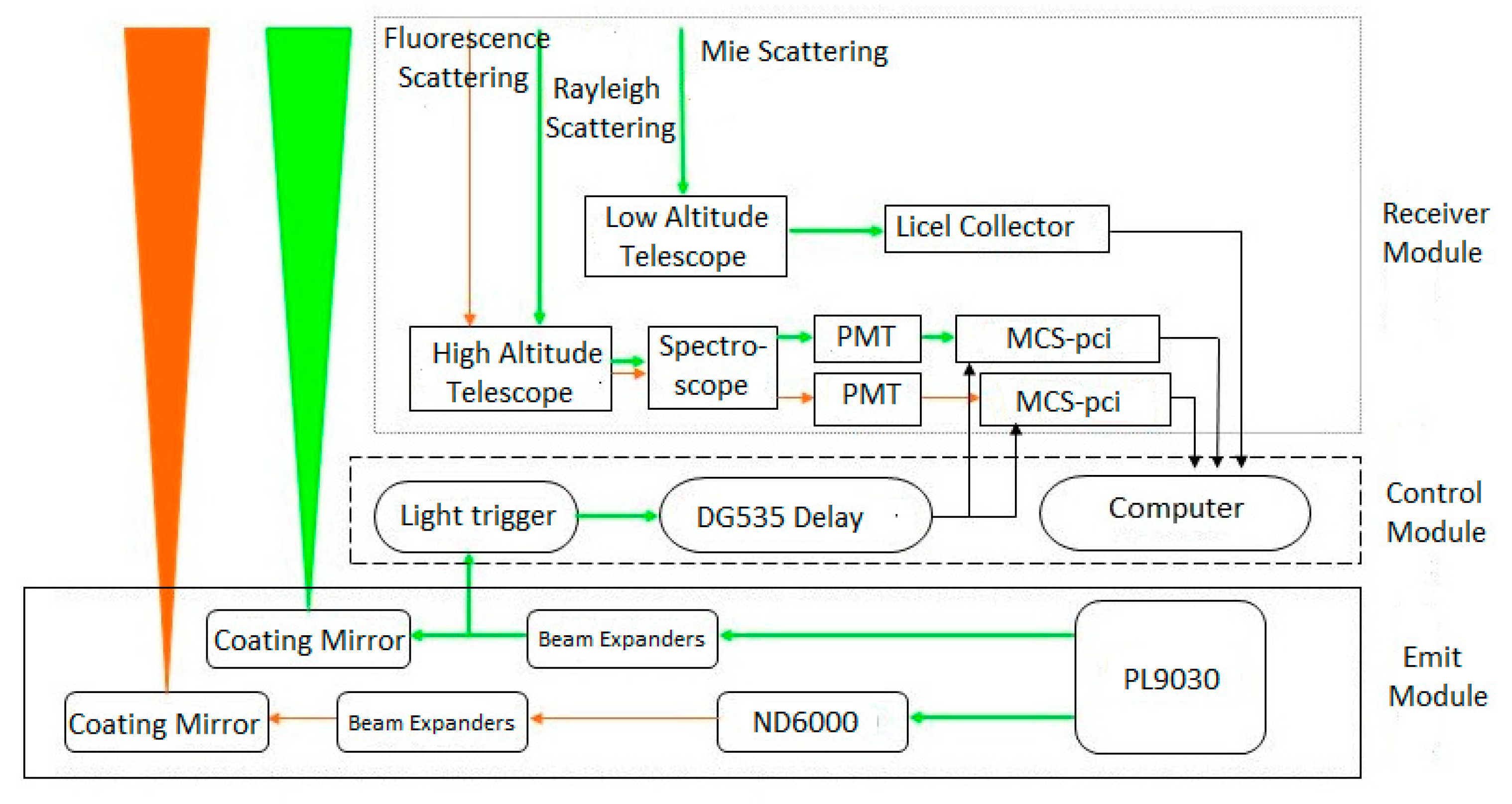
Based on the Rayleigh lidar observatory of the Meridian Project of China located in Beijing, China (40.5° N, 116.2° E), we were able to take the measurement of the original sodium density data in the lower MIL and further study the density and temperature variations of the middle atmosphere. The detailed characteristics of our lidar are presented in Figure 1 and

Table 1. Parameters of Rayleigh lidar in Beijing.

Transmitter	Nd:YAG Laser	DYE Laser
Wavelength	532 nm	589 nm
Pulse energy	320 mJ	60 mJ
Repetition rate	30 Hz	30 Hz
Pulse width	10 ns	10 ns
Beam divergence	<0.5 mrad	<0.5 mrad
Receiver
Telescope aperture	1 m
Field of view	1 mrad
Bandwidth	1.0 nm
Data acquisition
MCS-pci count rate	150 MHz
Bin width	640 ns

.

For our Rayleigh lidar, the two-channel (532 nm and 589 nm) detector that received signals from two lasers with different energy sources (320 mJ@532 nm, 60 mJ@589 nm) respectively was designed. Based on the multi-channel scalar (MCS) software, the backscattered signals could be processed, and the instrument accuracy was with a spatial resolution at 96 m and a temporal resolution of 166.7 s (5000 integrated laser shots). We refer to the method of Guan et al. [25] to calibrate the signal-induced noise (SIN) (Yue et al., 2014).

It is worth mentioning that our Rayleigh lidar could obtain the backscattered signals, which can help us acquire the atmospheric temperature information up to 85 km by the high-power aperture transceiver system, and the backscattered signals from two channels are used together to increase the dynamic range of the detector. The atmospheric density from 35 to 55 km was detected by the channel of 589 nm and those from 55 to 90 km were obtained by the 532 nm channel, which has a relative high sensitivity. The density profiles of 35–90 km and temperature profiles of the whole altitude range (35–85 km) could be calculated by choosing the NRLMSISE-00 [26] model data at about 60 km, and an initial temperature value from the NRLMSISE-00 model data was designated at 90 km, respectively. Based on the hydrostatic equation and ideal gas function (Hauchecorne and Chanin, 1980 [27]), we derived the data to obtain the temperature data. In this paper, the temperature profiles were retrieved from lidar observational data for over 130 nights from January 2012 to April 2013.

Since its inception on 7 December 2001, the Thermosphere Ionosphere Mesosphere Energetics and Dynamics (TIMED) satellite has worked for a period of 397 min and run at an orbit of 625 km above the earth ground with an inclination of about 74.1° from the equator. The SABER instrument is a 10-channel infrared (1.27–16.9 μm) radiometer onboard the TIMED satellite. For temperature measurements, three channels are used in the 4.3 and 15 μm CO₂ bands, and the vertical resolution was approximately 2 km in the stratosphere and mesosphere. The uncertainty of temperature is 1–3 K in the lower stratosphere, 1 K near the stratopause, and 2 K in the mesosphere and lower thermosphere (MLT) for the SABER v1.07 data set. In general, the SABER can provide the global viewing of the middle atmospheric thermal structure studies [15].

In this report, the SABER data of version level-2A publicly available on the http://saber.gats-inc.com/ website (last access: 9 September 2021) were used for analysis. The chosen plots for comparison were around Beijing, China (40.5° N, 116.2° E, the Rayleigh lidar site), which are within the latitude range 38–42° N and 115–138° E.

According to the theory, we calculate the density of the middle atmosphere as follows: due to the properties of Rayleigh lidar detection, the received laser signals were mainly reflected by molecule Rayleigh scattering by ignoring the atmosphere sol–gel. First, we fix an assumed height over 30 km, above which the atmosphere optical thickness is less than 0.01. By our programming, we can obtain the atmospheric density profile and eliminate the effect of the Rayleigh lidar system parameters and the atmospheric transmittance rate. Under the ideal atmosphere dynamics hydrostatic equilibrium and ideal gas equation of state shown below, the atmosphere temperature profile could be obtained [26].

$$\rho \left(z\right)=\rho \left(z^{*}\right)\frac{{\left(z\right)}^{2}N\left(z\right)}{{\left(z^{*}\right)}^{2}N\left(z^{*}\right)}$$

(1)

where z* refers to the reference height, and ρ (z) and ρ (z*) are the atmosphere density at z and reference height z*. In practice, we chose the reference atmosphere density by TIMED/SABER sources, and in this work, the reference height was defined at 60 km, and the reference density was provided by NRLMSISE-00; N(z) and N(z*) are atmospheric echo photon counts at z and z*, respectively.

$$T\left(z_i\right)=\rho \left(z^{*}\right)\frac{\rho \left(z_i\right)}{\rho \left(z^{*}\right)}·T\left(z^{*}\right)+\frac{1}{R}\underset{z}{\overset{z^{\prime }}{{\displaystyle \int }}}\frac{\rho \left(z^{\prime }\right)}{\rho \left(z_i\right)}·g\left(z^{\prime }\right)d{z}^{\prime }$$

(2)

where R denotes the universal gas constant, z* denotes the height of the boundary, ρ(z*) and T(z*) were the height of the upper boundary of the atmospheric density and temperature, which are usually given by the TIMED/SABER or atmospheric model NRLMSISE-00. As a sequence, it can be concluded that the density inversion error does not depend on the absolute value of the temperature but only relative with the density, temperature reference point, atmospheric transmittance, and echo signal strength. The accuracy of the atmospheric temperature inversion algorithm depends on the variations of the Rayleigh echo photons error, which could be considered consistent with the precision accuracy of approximate density and temperature inversion. Since the feedback photons are mutually independent and obey a Poisson distribution, it can be concluded that the temperature inversion derivation error is inversely proportional to the square root of the number of the received photon counts. We also provide the derivation error data around 80 km in the supplementary information, which is usually considered to be where large temperature errors happened.

3. Results

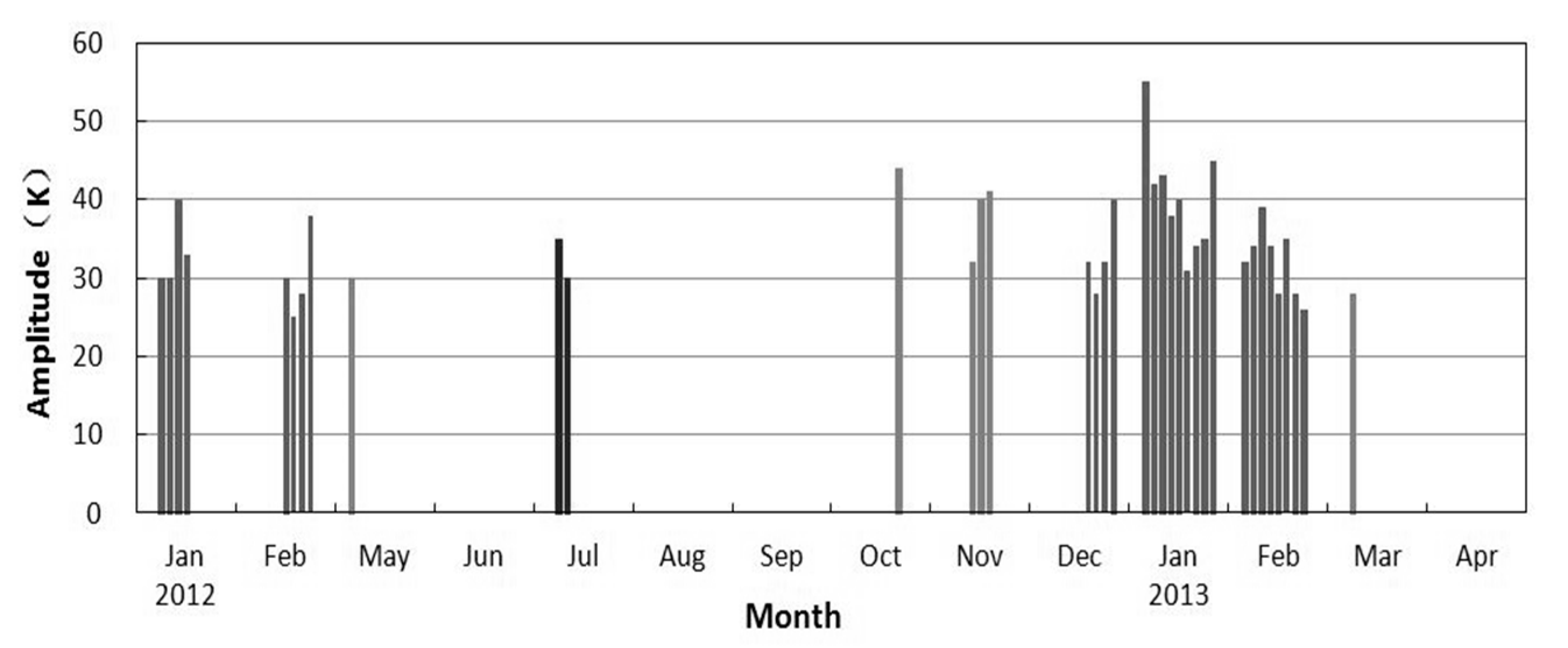
Those occurrences of temperature inversion amplitudes of MIL have been statistical as Figure 2 shows, and it can be concluded that those temperature inversion amplitude data ≥ 25 K mainly occur in winter, and the maxima inversion amplitude also appears in the winter season. During the spring and summer, the occurrence of the inversion amplitude ≥ 25 K MIL phenomenon was the lowest. While in the autumn, the occurrence and the maximum inversion range is a little larger than those in the spring and summer. After statistics, the averaged inversion temperature range of the low MIL is calculated as 23.4 K, and the average range of the layer thickness is 4.78 km with an averaged MIL bottom altitude of 68.2 K. Among those 91 phenomena of the lower MIL, about 50% of the vertical propagation phenomena over time occurred at the inversion layer bottom (top) by statistics. In addition, 47 low-level MIL events spread downward, while 12 low-level MIL events have been observed spreading upwards, which indicated that the number of upward propagation MIL events occurred much more frequently than the lower MIL events that spread downward.

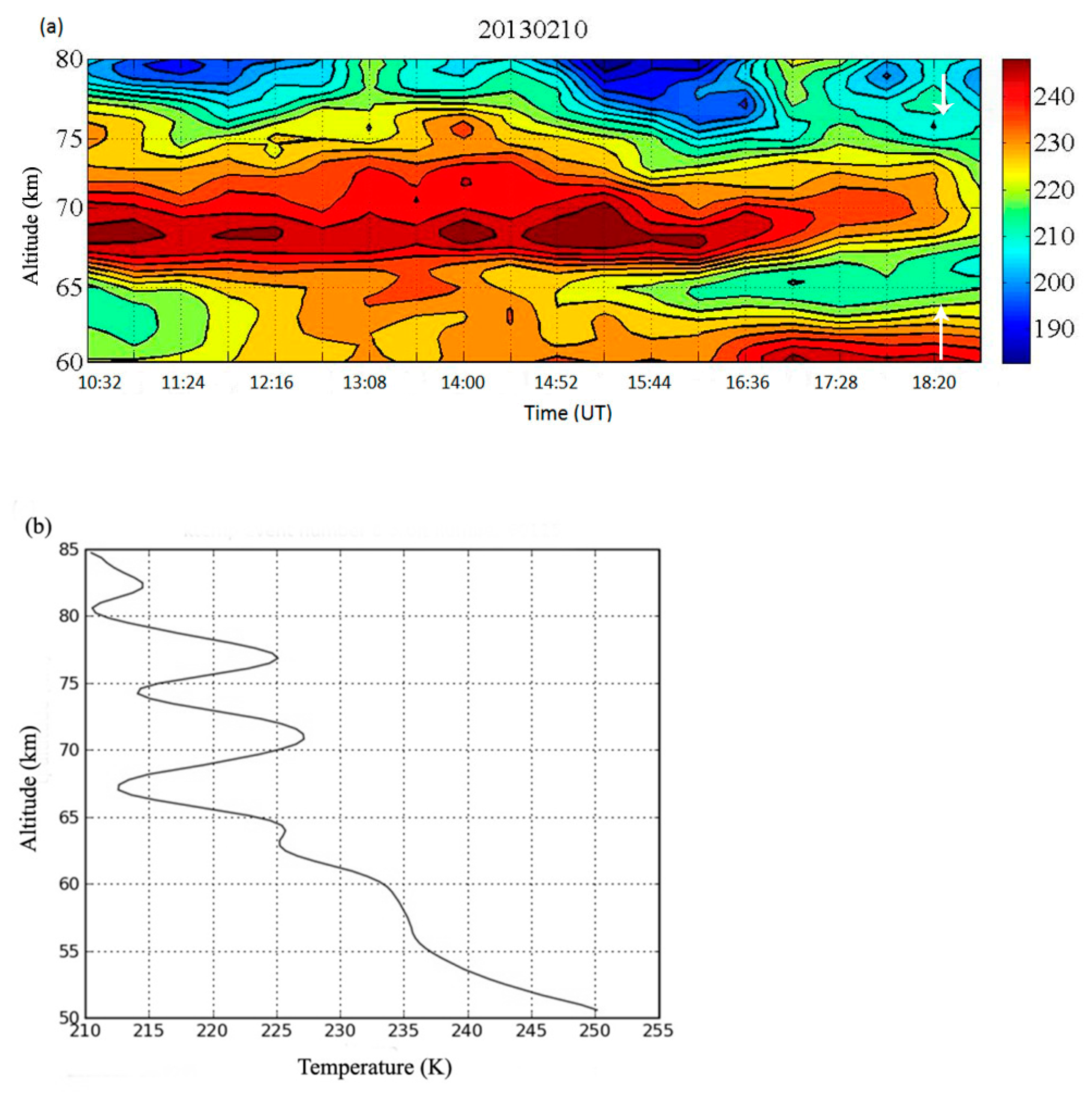
As shown in Figure 3, a typical lower MIL case occurred on 10 February 2013. An apparent MIL emerged at 10:32 UT at around 63 km, and this slow MIL propagation lasted for 5 h (16:33 UT). The total inversion layer thickness is 4 km with a temperature inversion amplitude of 25 K, which increased gradually later over 30 K, and the inversion layer thickness also increased with a relative high velocity at 710 m/h. Another small MIL with a relatively small temperature inversion amplitude of about 10 K emerged at 18:23 UT, whose top was at 76 km (as the white arrows indicated), but this MIL had a very small duration time, which lasted only 10 min in total, and the vertical thickness was about 1 km. The reference TIMED/SABER data on the same date at (38.0° N, 137.9° E) provided on website http://saber.gats-inc.com (last access: 9 September 2021) is shown in Figure 3b, which shows the relative MIL cases with the 4 km thickness and the bottom layer latitude at 63 km, which are reasonably consistent with our Rayleigh lidar observation results.

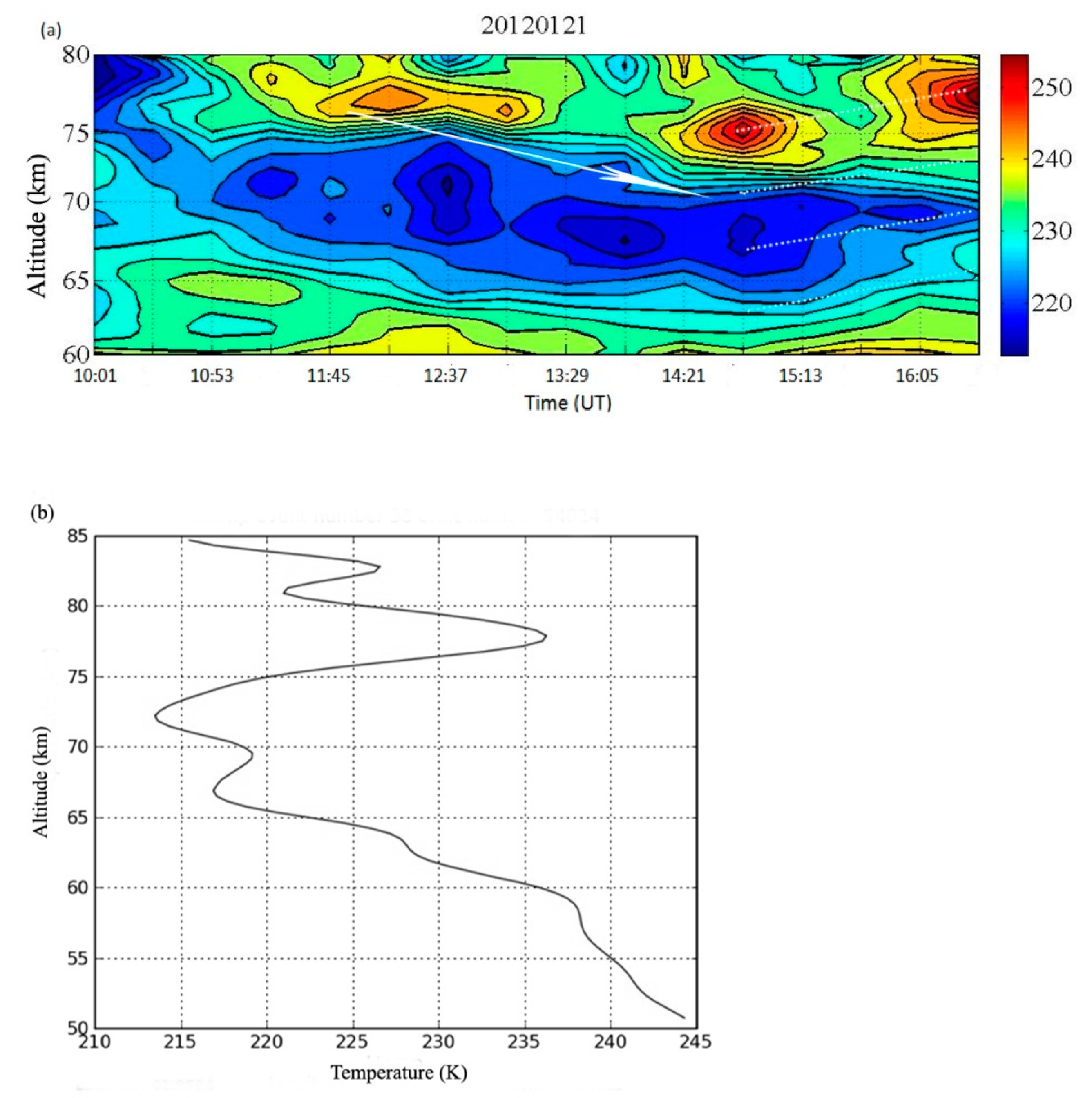
Figure 4a shows an unusual case on 21 January 2012 in which the high MIL propagated downward and combined with a newly emerged low MIL event. As Figure 4a shows, an apparent high MIL emerged at 10:32 UT at around 72 km and propagated upward as a velocity of 500 m/h and gradually enlarged. While at 12:37 UT, another low MIL whose center was at 71 km emerged and propagated downward obviously, while the high MIL at the same time did not stop its downward propagation (as the white arrows indicated), and it combined with the low MIL at 13:29 to form a considerable MIL with a huge vertical thickness of 10 km and a temperature inversion amplitude of 26 k. It was worth mentioning that another abnormal phenomenon happened at 16:20 in which the newly occurred high MIL combined with the previous downward propagated MIL, which had a high temperature inversion rate and a tendency to propagate upward (as the dashed line indicated). This phenomenon is seldom reported among those observed cases compared to the previous studies. The TIMED/SABER data on the same date at 41.9° N, 119.7° E are shown in Figure 4b, which shows the relative MIL cases with about 8 km thickness between about 70 and 80 km and the relative huge temperature inversion amplitude at 25 k. The high MIL over 80 km also could be observed with a small thickness of about 2 km, as indicated in the SABER data, which also partly suit our Rayleigh lidar observation results due to the possible error of observation site temporally and spatially.

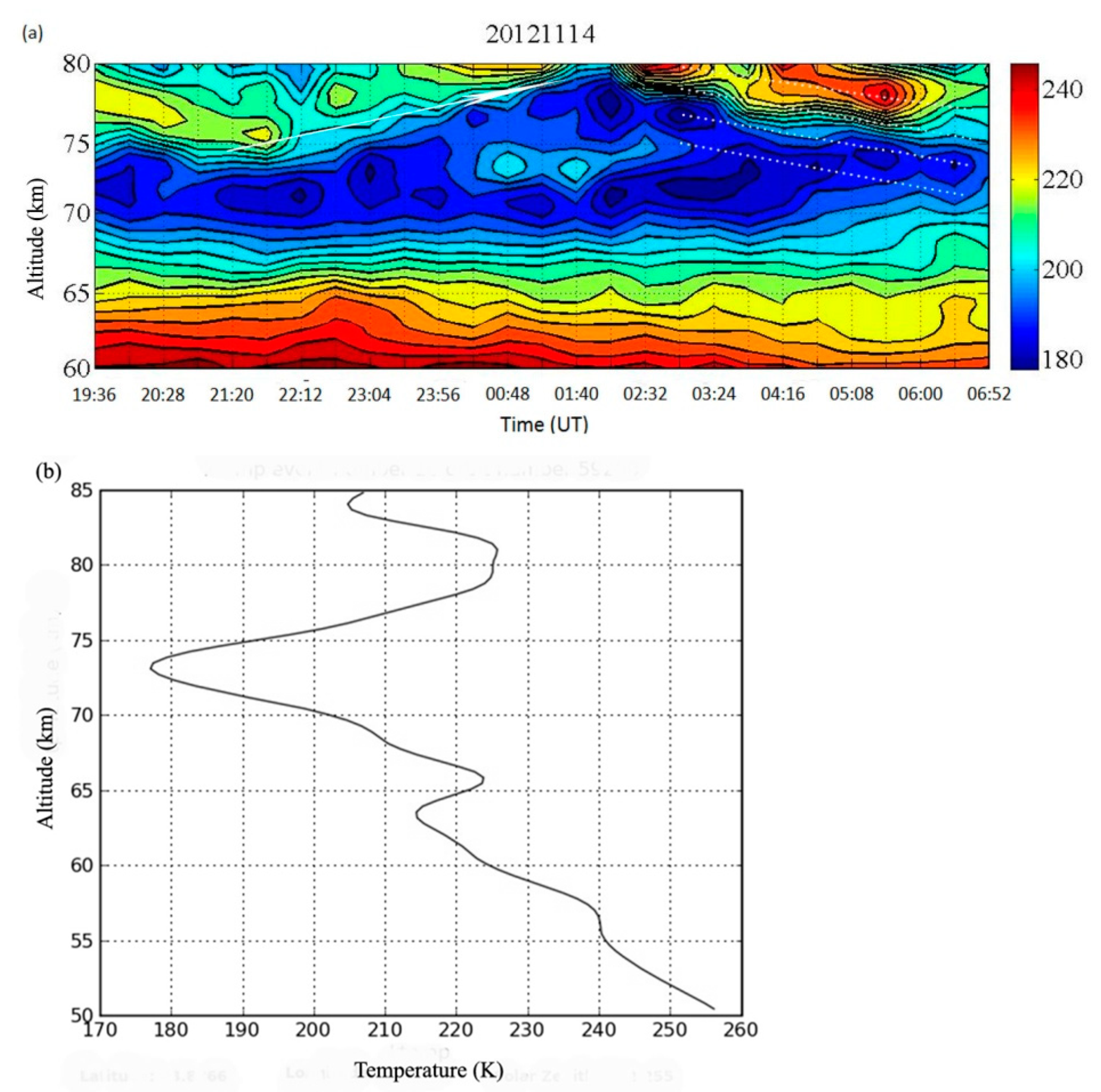
A single MIL divided into a bi-MIL and dissipated phenomenon has been also observed, as shown in Figure 5a. On 14 November 2012, at 19:36 UT, an MIL at 72–77 km occurred with a temperature amplitude of 23 K. This MIL emerged and propagated first downward slightly for about 2 h and then transformed to propagate upward (as the white arrows indicated) to the high mesosphere with a vertical velocity of 1430 m/h and the thickness enlarged gradually to a range of 8 km and even reached above 80 km. Then, at 00:48 UT, the MIL divided into two parts to form a bi-MIL of 70–72 km and 72–80 km, and the MIL of 70–72 km lasted for about 2 h and then recombined with the upward propagating 72–80 km MIL (as the dashed line indicated) to form the new MIL with an inversion temperature over 30 K and continued to propagated downward rapidly with a velocity of 750 m/h. Duck et al. [23] reported a lower MIL downward transmitting case with a velocity of 400 ± 60 m/h, which is similar to the result on 12 January 2012, and the observed velocity of 1480 m/h was much faster than that of Duck et al. [23]. As Figure 3 shows, the propagation velocity of the case observed before was about 710 m/h, and one case on 8 February 2013 was observed at a velocity of 200 m/h, which is 50% of Duck’s report, indicating that the propagation velocity in Beijing has larger individual differences.

The reference TIMED/SABER data on the same date at 41.9.0° N, 119.7° E as shown in Figure 5b show the relative MIL cases with a relatively long thickness at 8 km between about 73 and 80 km and the relative huge temperature inversion amplitude at 25 K, and moreover, the MIL between 78 and 82 km may reflect this combination and propagation, which may support our report.

4. Discussion

During our 139 observing days, we have statistically 91 low-MIL cases or 65% in total, which is similar to the result of 67% given by Fadnavis and Beig (2004) observed in India tropical regions, and less than the 70% percentage reported by Leblanc and Hauchecorne in South France (44° N, 5° E) [6]. Due to the higher resolution of our equipment, the standard temperature detection of 70 km causes the error to be less than half that of Leblanc and Hauchecorne’s report, and furthermore, the average MIL temperature is 23.4 K, which is slightly lower than the reference temperature 25 k of their report [6].

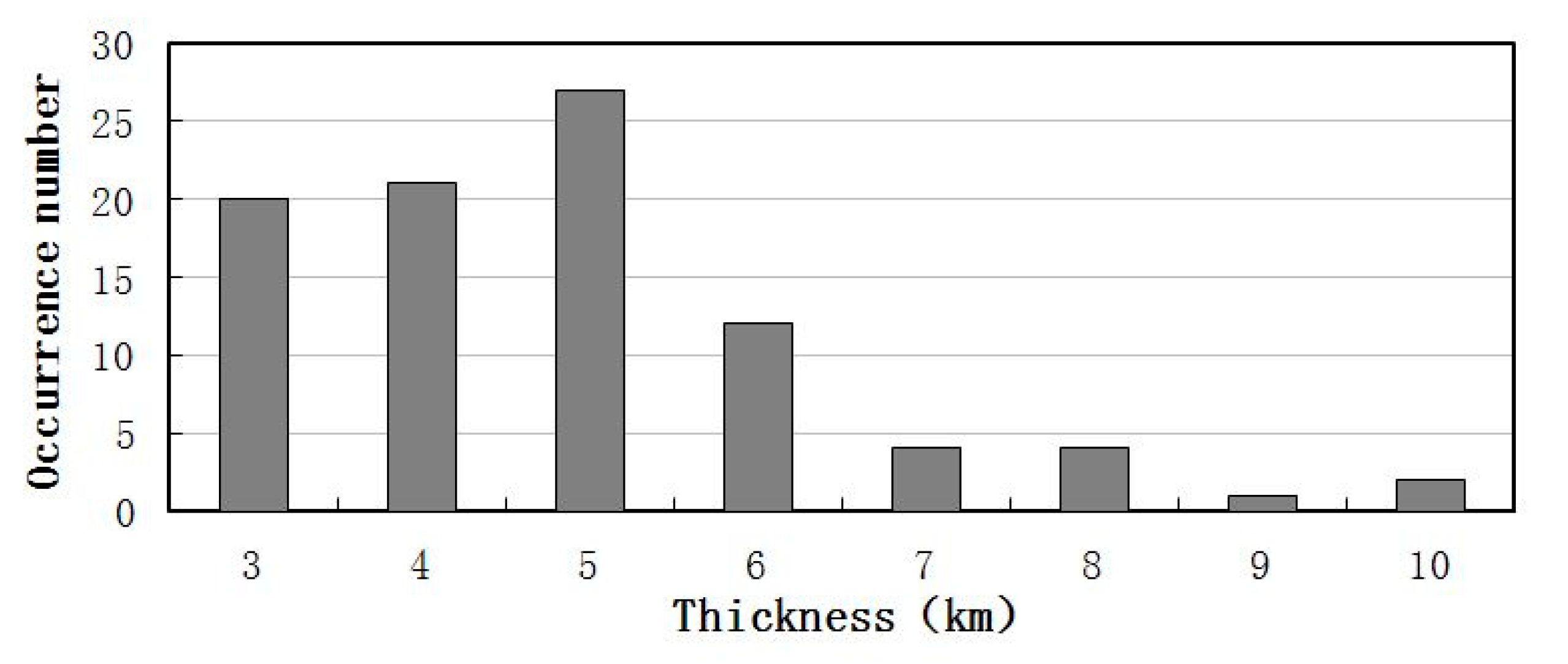
It also indicates that among the observed 91 lower MIL cases, the thickness of the MIL mainly distributed from 3 to 6 km, as shown in Figure 6, and those cases for which the MIL thickness was 3 km emerged 20 days at a considerable high frequency. This result shows a relative significance compared to the previous report (Fechine et al., 2008) that ignored this in lower MIL analysis [1]. Further study shows the average height of the bottoms of the MIL whose thickness is 3 reach to 69.2 km, and the inverse temperature range is 18.3 K, which indicates a contrary result to the previous reports (Fechine J. et al., 2008) [1]; i.e., the average height of the bottom boundary of lower MIL is higher than those of similar phenomena, and the temperature amplitude is lower as well. Salby et al. [28] reported that the large-scale circulation distortion under the influence of planetary waves will cause temperature inversion temporally and spatially, and those of the smaller-scale MIT may be caused by gravity waves. Later, Ramesh et al. indicated that the main mechanism of the MIL can be ascribed to the gravity wave breaking, and the amplitude of MIT are affected by the gravity wave and planetary waves interactions [18]. For the Beijing area, the large-scale mesosphere cooling and large-scale MIL and stratosphere sudden warming happened from November 2012 to January 2013, during which the first planetary wave enhanced significantly in the mesosphere, as Yue et al. [15] and Hoche et al. [14] indicated. Moreover, gravity wave and planetary waves interactions always exist, and other complex chemical and dynamical processes in the mesosphere could lead to these MIL cases; nevertheless, more further studies and joint observations are needed due to the lidar detecting limitation.

5. Conclusions

Based on the Rayleigh lidar observatory located in Beijing, China (40.5° N, 116.2° E) that was established in the Meridian Space Weather Monitoring Project of China, an advanced Rayleigh lidar observation system was introduced. Typical lower MIL cases were first reported based on 139 Rayleigh lidar data and comparison with the SABER data; the seasonal distribution of lower MIL cases were calculated, and the reason for these cases were discussed. The special low MIL phenomenon may be caused by interactions between gravity waves and planetary waves. For the Beijing area, there is large-scale mesosphere cooling and large-scale MIL and stratosphere sudden warming. These results discover the properties of temperature behavior of the lower MIL over North China, which may be helpful for us to further understand middle atmosphere chemical and dynamics processes.