Article

Investigation of Volcanic Emissions in the Mediterranean: “The Etna–Antikythera Connection”

1
National Observatory of Athens/IAASARS, 10560 Athens, Greece
2
Department of Meteorology and Climatology, School of Geology, Aristotle University of Thessaloniki, 54124 Thessaloniki, Greece
3
Research Centre for Atmospheric Physics and Climatology, Academy of Athens, 10680 Athens, Greece
4
Laboratory of Atmospheric Physics, Physics Department, Aristotle University of Thessaloniki, 54124 Thessaloniki, Greece
5
German Aerospace Center (DLR), Institute of Atmospheric Physics, Oberpfaffenhofen, 82234 Weßling, Germany
6
Consiglio Nazionale delle Ricerche, Istituto di Metodologie per l’Analisi Ambientale (CNR-IMAA), 85100 Potenza, Italy
7
Istituto Nazionale di Geofisica e Vulcanologia, Osservatorio Etneo, 95100 Catania, Italy
*
Author to whom correspondence should be addressed.
Atmosphere 2021, 12(1), 40; https://doi.org/10.3390/atmos12010040
Submission received: 10 December 2020 / Revised: 24 December 2020 / Accepted: 28 December 2020 / Published: 30 December 2020
(This article belongs to the Special Issue Evaluation and Optimization of Atmospheric Numerical Models)

Abstract

:
Between 30 May and 6 June 2019 a series of new eruptions occured in the south-east flanks of Mt. Etna, Italy, forming lava flows and explosive activity that was most intense during the first day of the eruption; as a result, volcanic particles were dispersed towards Greece. Lidar measurements performed at the PANhellenic GEophysical observatory of Antikythera (PANGEA) of the National Observatory of Athens (NOA), in Greece, reveal the presence of particles of volcanic origin above the area the days following the eruption. FLEXible PARTicle dispersion model (FLEXPART) simulations and satellite-based SO2 observations from the TROPOspheric Monitoring Instrument onboard the Sentinel-5 Precursor (TROPOMI/S5P), confirm the volcanic plume transport from Etna towards PANGEA and possible mixing with co-existing desert dust particles. Lidar and modeled values are in agreement and the derived sulfate mass concentration is approximately 15 μg/m3. This is the first time that Etna volcanic products are monitored at Antikythera station, in Greece with implications for the investigation of their role in the Mediterranean weather and climate.

Graphical Abstract

1. Introduction

Volcanic eruptions can inject huge amounts of particles and gases into the atmosphere, which can have an important impact on regional and global scale [1,2,3]. Volcanic emissions are composed by volcanic particles generated by magma fragmentation and gases. The most abundant is the sulfur dioxide (SO2) which is oxidized by the hydroxyl radicals (OH) to form sulfate aerosols in the atmosphere [4,5]. Through kinetic-based simulations, high-temperature chemistry quickly forms oxidants, such as OH, HO2, and H2O2, can lead to the production of sulfate within a few seconds after the emission of SO2 begins. The oxidation of SO2 and hydrogen sulfide (H2S) gases generates submicron sulfate particles with a lifetime of several years if those are injected in the lower stratosphere or in the upper troposphere, and from days to a few weeks if those are injected in the troposphere [1]. In the absence of clouds, the photochemical SO2 conversion to sulfate particles proceeds more rapidly during the day and in the summer (5–10% h−1 SO2 conversion rate) than during the night and in the winter (0.3–1% h−1). The rate of conversion depends on the nature of the surface, the presence of co-pollutants, the temperature, and the relative humidity. In addition, if the plume has a high dust/ash density then heterogeneous surface reactions may play a significant role [6]. Hobbs et al. [7] observed oxidation rates in the Mt. St. Helens plume that were comparable to those observed in power-plant plumes (0.1% h−1). A minimum of 13 Tg/y of time-averaged SO2 fluxes has been reported by actual volcanic measurements worldwide during the period 1970–1997 [8]. Τhe global SO2 budget from volcanoes has been recently revised to about 23 ± 2 Tg/yr, for the period 2005–2015, based on spaceborne observations from the Ozone Monitoring Instrument (OMI) onboard NASA’s Aura satellite [9]; The contribution of volcanoes to the total sulfur emissions in the atmosphere is up to 10% [10]. Remarkably, volcanic emissions also have a bigger impact on the tropospheric aerosol burden than other sulfur sources [11] because volcanoes tend to emit SO2 at higher altitudes than most other surface sulfur emissions, where the lifetime is longer [12].
The impact of volcanic emissions on the planetary radiative budget is further intensified when volcanic eruptions inject particles in the stratosphere. The long residence time in the stratosphere accompanied by the strong interactions between both ash and sulfates with solar radiation increase the Earth’s albedo and can cause ozone depletion on a global scale (e.g., at Mt. Pinatubo massive eruption in 1991, record-low ozone abundances were observed over much of the northern hemisphere) [1,13,14]. Earlier research has broadly considered two major aerosol sources in the stratosphere, namely, the direct injection of ash and sulfates by volcanic eruptions and the isentropic transport of carbonyl sulfide [15,16,17].
Additionally, volcanic material injected and transported at flight altitudes similar to dust and smoke [18] poses a serious hazard to aviation since it can cause damage and loss of power of the aircraft engines [19,20,21]. Ash particles can lead to dangerous aircraft engine damage, and products of SO2 have highly corrosive properties [22]. Despite the importance of this process to emergency responders and aviation, the operational systems capable of monitoring tephra dispersal and fallout in near-real-time, and subsequently provide the expected impact assessment are still limited and not fully adapted to the growing requirements of precision and reliability [23].
Forecasting the transport of volcanic plumes for aviation hazards mitigation requires timely analysis of all available observations to initialize and refine ash dispersion forecasts and issue Volcanic Ash Advisories in the wake of a volcanic eruption [24,25]. A variety of satellite sensors which have been used over the past decades, like the TROPOspheric Monitoring Instrument onboard the Sentinel-5 Precursor satellite (TROPOMI/S5P) [26], can detect volcanic plumes. The TROPOMI imaging spectrometer represents a step-change in gas monitoring from space as it measures in four different spectral regions (UV-visible, near-infrared, shortwave infrared), providing volcanic SO2 vertical column density (VCD) maps at an unprecedented spatial resolution, used to track the horizontal transport of volcanic SO2 clouds [27]. Observations from both satellites and ground-based lidar instruments have been used to monitor and track the altitude and properties of volcanic aerosols [28,29,30].
In the days following a volcanic eruption, SO2 and ash particles are injected in different heights and may take different transport pathways, as a result of the varying vertical and horizontal wind shear [31,32]. Modeling and forecasting the transport and atmospheric concentrations of volcanic aerosol released during volcanic eruptions (e.g., SO2) depend critically on the knowledge of the eruption source term. Unfortunately, the estimation of the source term is difficult to obtain by direct measurements and often relays on ground-based remote systems as video-surveillance systems (e.g.,[33]). The main source term of an eruption includes parameters like the release height, the total mass, the mass eruption rate, and the duration of the eruption [34]. An additional parameter describing ash emissions in particular is the particle size distribution that among the input parameters is one of the most difficult parameters to measure in real time [23].
Long-range transport of volcanic aerosols over the Mediterranean is recorded systematically by the European Aerosol Research Lidar Network (EARLINET) (e.g., [35]). Recent observations from the newly established PANhellenic GEophysical observatory of Antikythera (PANGEA) of the National Observatory of Athens (NOA) during the period 30 May–6 June 2019 depict the transport of elevated layers above the Eastern Mediterranean. The presence of these elevated layers is mostly associated with the continuous Etna volcanic activity.
The aim of this study is to investigate the properties of Etna volcanic emissions and their transport paths in the Mediterranean. Mt. Etna is the largest point-source of particulate matter in the atmosphere of the Mediterranean, affecting the atmospheric levels of airborne particles and their deposition rates at both local and regional scales [36,37,38]. For this purpose, we combine satellite observations and modeling tools as well as ground-based remote sensing near the volcano and at the remote island of Antikythera located 765 km downwind of the volcano.
The manuscript is organized as follows: in Section 2 we present the case study of the 30 May–6 June 2019 eruption of Etna, the atmospheric circulation and the transport pathways between Etna and the Antikythera station. In Section 3 we introduce the methodology used in our analysis to describe the long-range transport of Etna emissions. In Section 4 we present the results obtained by applying the methodology. The transport of the volcanic SO2 plume is simulated with the Lagrangian particle dispersion model FLEXPART and it is validated with data from the Modern-Era Retrospective analysis for Research and Applications version 2 (MERRA-2 reanalysis) and remote sensing observations (PollyXT lidar, TROPOMI/S5P). Finally, in Section 5 we present our conclusions and indicate directions for future work.

2. The Case of 30 May–6 June 2019 Etna Volcanic Eruption

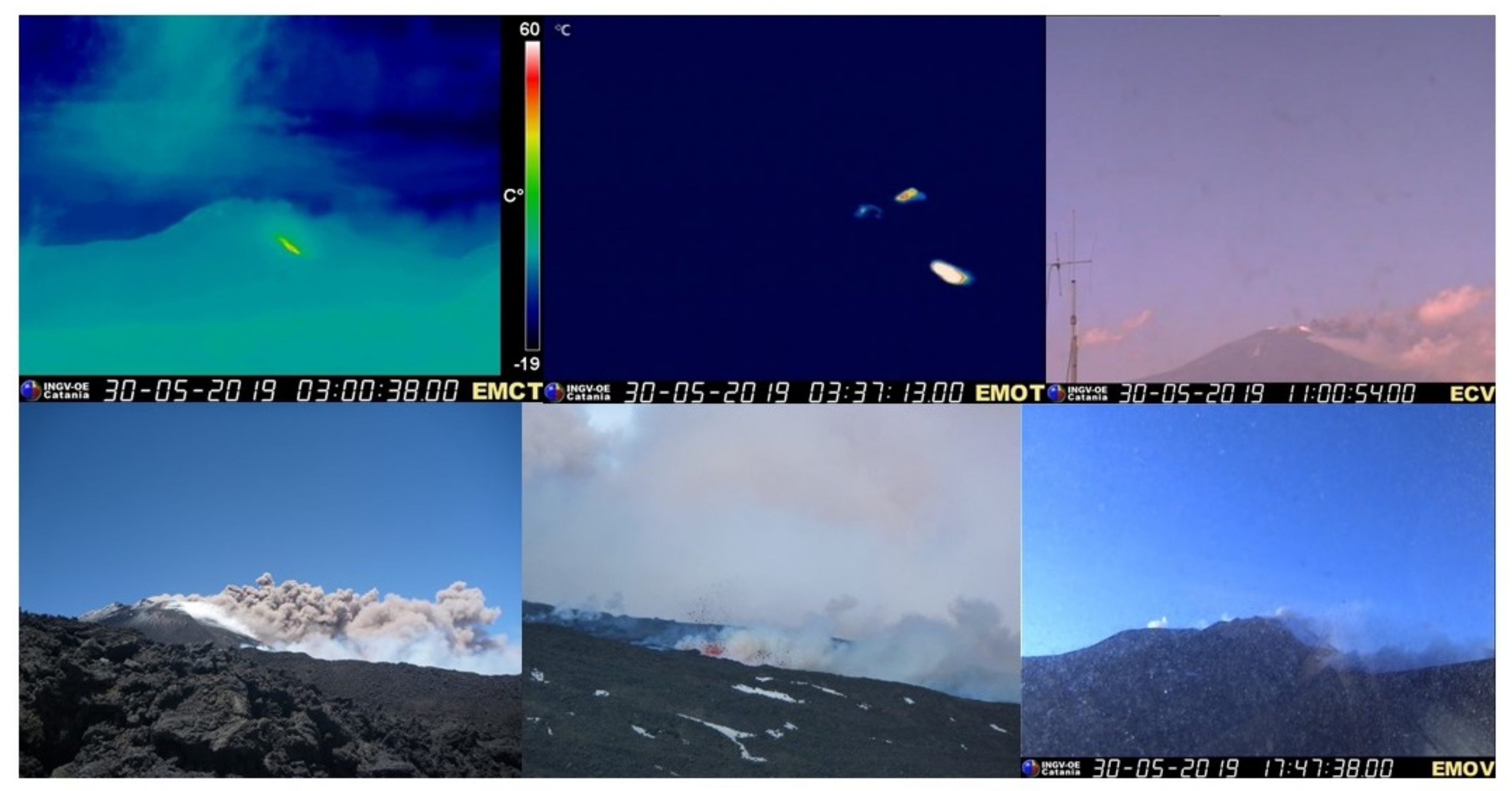
2.1. Volcanic Activity/Emissions

The Mt. Etna volcano (37.74° N, 15.00° E, 3300 m above sea level (a.s.l.)) is located in Sicily, Italy, and is one of the most active volcanoes on Earth. This active stratovolcano has historically recorded eruptions over the past 3500 years while it has been erupting periodically since September 2013 to this day. Lava flows, explosive eruptions with ash plumes, and Strombolian lava fountains commonly occur from one or more of its summit craters named Voragine (VOR), Northeast Crater (NEC), Bocca Nuova (BN), and Southeast Crater (SEC). In the latter, recent activity is located on a new cone formed since 2011 on the volcano’s eastern flank, namely the New Southeast Crater (NSEC), [39,40,41,42].
On 1 May 2019 the Istituto Nazionale di Geofisica e Vulcanologia, Osservatorio Etneo (INGV-OE) reported Strombolian activity from the BN crater, followed the day after by Strombolian activity at the NSEC. The activity from the summit craters was almost constant, often forming dilute ash emissions that were dispersed quickly by winds. On 29 May 2019, late in the afternoon, there was an increase of volcanic tremor that preceded the new flank eruption. On 30 May 2019 lava flow and explosive activity at the east base of NSEC were in fact observed from the video-surveillance system of INGV-OE since about 01:30 UTC and a new lava flow formed after about two hours on the south flanks (Figure 1). Intense ash emission was dispersal toward the northeast and decrease in intensity in the afternoon (Figure 1). Lava flow from the fracture opened on the east flank stopped late in the afternoon of 1 June 2019 while lava flow emission and light explosive activity went on from the south fissure. This latter drastically decreased on 4 June 2019 and definitively stopped on 5 June 2019, while effusive activity ceased in the morning of 6 June 2019.
According to the Volcano Observatory Notice for Aviation (VONA) messages, the volcano observatory issued a warning report, from yellow to orange levels, early in the morning of 30 May 2019 while a red alert was issued from 10:50 UTC to 17:29 UTC when a strong ash emission was observed.
TROPOMI/S5P instrument SO2 retrievals provided the same information (Figure A1). By this time, lava flows and explosions had produced persistent SO2 plumes that drifted east and north east for over 800 km from the source, as seen by TROPOMI/S5P (Figure A1). This volcanic activity did not result in any major air traffic disruption.
The TROPOMI/S5P polar orbiting instrument produces daily global SO2 VCD maps (Figure A1). It represents the amount of SO2 molecules in a column overhead per unit surface area generally expressed in Dobson Units (1 DU = 2.68 × 10¹⁶ molecules SO2 cm−2). From the SO2 VCs, one can easily calculate the total SO2 mass for a given area (e.g., Figure A1) which is a quantity useful to investigate volcanic activity [43].

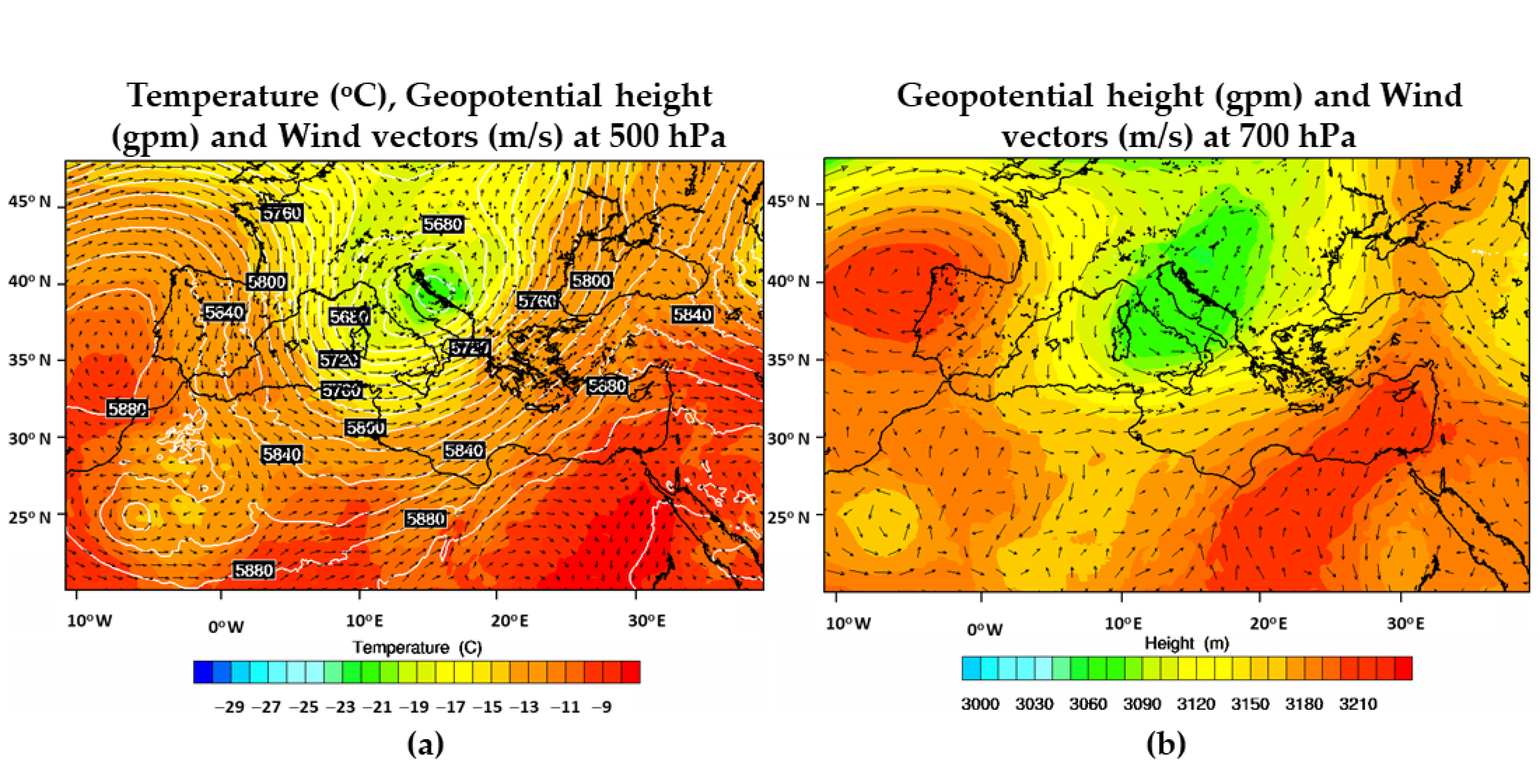
2.2. Atmospheric Circulation and Transport Pathways

The atmospheric circulation over the eastern Mediterranean is dominated by persistent northerly and westerly winds, favoring the advection of volcanic products from Etna to Greece [44]. In order to demonstrate the strong connection between Mt. Etna volcano air masses and the PANGEA-NOA station HYSPLIT cluster analysis was performed for a five-year period. The HYSPLIT (Hybrid Single-Particle Lagrangian Integrated Trajectory) model was used to compute air parcel trajectories of long-range transport [45] driven by the 6-hourly meteorological dataset Global Data Assimilation System (GDAS) at a resolution of 1° × 1° for a five-year period (2015–2019). During this five-year period, the Mt. Etna volcano has erupted about 50 times according to INGV reports, but this analysis is assessed by the overall contribution of air masses and not only when Etna erupted within this time.
A two-step cluster analysis was applied to the 48-h forward trajectories starting from Mt. Etna volcano to investigate the emissions transport pathways. The first step involves the clustering of 48 h of forward trajectories at six height levels, 3300 m, 5000 m, 7500 m, 10,000 m, 15,000 m, and 18,000 m above ground. In the second step, clustering analysis was applied for the selected period at each of the height levels, to 1816 in total forward trajectories.
The cluster analysis indicates that due to the synoptic circulation characteristics of the Mediterranean, a significant proportion of tropospheric air masses from Etna volcano are transported eastward towards the island of Antikythera, where the PANGEA station is located. For the five years period examined here the percentage of eastward trajectories starting at each HYSPLIT height are 42% for 3.3 km, 43% for 5 km, 65% for 7.5 km, 63% for 10 km and up to 70% for 15 and 18 km. Thus, the predominant transport pattern highlights the strategic location of PANGEA observatory in monitoring volcanic emissions and establishing the so-called here “Etna–Antikythera connection” (Figure 2).

3. Experimental Design

Our methodology for the analysis of Etna volcanic plume transport for the specific case study of May–June 2019 flank eruption, incorporates the use of a number of numerical modeling systems, namely, the Lagrangian particle dispersion model FLEXPART coupled with the state-of the-art Weather Research and Forecasting model (WRF-ARW), along with MERRA-2 Reanalysis simulations. In addition, PollyXT NOA lidar data from the PANGEA station and satellite observations from the TROPOMI/S5P are utilized.

3.1. Modeling

The transport of volcanic ash and SO2 plumes was simulated with the Lagrangian particle dispersion model FLEXPART [3,46,47] in a forward mode. Additionally, for the characterization of air masses and for the observed aerosol layer identification, the FLEXPART-WRF model was used in backward mode for the computation of source-receptor relationships, as well as back-trajectories, with a total of 10,000 particles released at heights 0.5, 1, 1.5, 2, 2.5, 3, 3.5, 4, and 4.5 km over the Antikythera station. FLEXPART has been used in a large number of similar studies on long-range atmospheric transport including volcanic plumes [3,48,49].
For the description of the event, the dispersion simulations were driven by hourly meteorological fields from the Advanced Research WRF (ARW) model version 4 [50]. The WRF-ARW spatial set up was at 9 × 9 km resolution domain with 600 × 370 grid points and 33 vertical levels. Simulations were initiated at 00:00 UTC on 30 May 2019 and were completed at 00:00 UTC on 4 June 2019. Table 1 summarizes the Physics Parameterizations (PP) schemes for the WRF-ARW simulations. The initial and boundary conditions for the offline coupled FLEXPART-WRF runs are taken from the European Centre for Medium-Range Weather Forecasts (ECMWF) Integrated Forecast System (IFS) operational analyses with 0.18° × 0.18° resolution and 91 model levels. Sea Surface Temperature (SST) analysis data were provided by the Copernicus Marine Environment Monitoring Service (CMEMS) at a resolution of 1/12°. The use of 1-hourly WRF meteorological fields at a 9 × 9 km spatial resolution allows a more detailed representation of the volcanic plume dispersion.
For SO2, a range of different values for the mass released were used in the model simulations following previous studies in order to select the more realistic one. Coppola et al. [51] incorporating satellite-based observations showed that the average SO2 flux of the Mt. Etna volcanic activity between 2004 and 2010 was equal to 3259 tonnes per day [51]. Granier et al. [52] estimated the average SO2 emissions for 2005–2010 of Mt. Etna volcano to 3456 tonnes per day using data from the NOVAC (Network for Observation of Volcanic and Atmospheric Change) network. In addition, Queißer et al. [27] made a comparison of SO2 fluxes, of one month from TROPOMI/S5P from the automated scanning FLux Automatic MEasurments (FLAME) ground-network, and fluxes from driving traverse measurements underneath the volcanic plume. An excellent agreement was shown for most of the days demonstrating that reliable, nearly real-time, high temporal resolution SO2 flux time series from TROPOMI/S5P measurements are possible for Mt. Etna. The average monthly SO2 flux from TROPOMI/S5P was 2.83 ± 1.66 kt/day while for FLAME 2.39 ± 1.09 kt/day.
On 3 June 2019, at ~11:43 UTC, TROPOMI/S5P recorded total SO2 VCD values of approximately 1.17 ± 1.02 DU (about 33.48 ± 29.19 mg/m2), over Antikythera (see Section 3.3 for details). In this study, in order to calibrate the volcanic SO2 mass flux according to the TROPOMI/S5P values measured over Antikythera, we did recursive runs with the FLEXPART-WRF model with the emission rates over Etna ranging between 2 and 5 kt/day. A value of 4 kt/day which is an average of SO2 emissions of Mt. Etna volcano, was finally selected as in this case the model simulations matched the TROPOMI/S5P SO2 plume patterns over the area and the measured SO2 columnar concentrations over the Antikythera station. We present here the results obtained by simulations with SO2 emissions rates equal to 4 kt/day, emitted from the reported start time of the eruption until 4 June 2019, 00:00 UTC, when the volcanic activity on the SE base of Etna’s NSEC started to decline in frequency.
Table 1. Configuration of the Physics Parameterizations (PP) schemes for the WRF-ARW simulations.
PPSchemesReference
Microphysics (MP)Thompson[53]
Surface Layer (SFL)Monin–Obukhov (Janjic Eta)[54]
Planetary Boundary layer (PBL)Mellor–Yamada–Janjic (MYJ)[55]
Cumulus Parameterization (CUM)Tiedtke[56]
Longwave & Shortwave Radiation (RAD)Rapid Radiative Transfer Model (RRTMG)[57]
Land Surface (LSM)NOAH[58]
Ash particles simulations were initiated at the reported start time of the eruption on 30 May 2019 and were completed at 17:30 UTC on the same day, at the eruptive stage. Neither TROPOMI/S5P nor other satellite instruments such as the Ozone Monitoring Instrument [59] on board NASA’s Aura spacecraft [60] and the Ozone Mapping and Profiling Suite Nadir Mapper (OMPS-NM) on board the NASA-NOAA Suomi National Polar-orbiting Partnership (Suomi-NPP) [61] could detect any clear ash cloud. The detection of ash by satellite instruments is more complicated than that of SO2 because of the varying physicochemical properties of the ash particles (different size, geometrical shape, and composition) [62]. The mass eruption rate is usually estimated from the observed injection height with empirical relationships [23,34,63].
In our study we estimate the mass eruption rate (MER) for ash particles following Scollo et al. [23] study, by inverting the observed plume height using the 1-D plume model of Degruyter and Bonadonna [63]. Similar models are commonly used, as they can capture the first-order physics of a volcanic plume rising in the atmosphere, while remaining computationally efficient [64]. The Degruyter and Bonadonna [63] plume model assumes that (i) the plume is in a steady-state, (ii) the solid particle and gas phase in the plume are well mixed, such that they have the same bulk velocity and temperature, (iii) differences in pressure between the plume and the atmosphere are negligible and the velocity and temperature distributions through a cross-section of the plume follow a top-hat profile, which remains self-similar along the plume trajectory [23,63]. The mass eruption rate from plume height was calculated according to Equation (1):
M ˙ = π ρ α 0   g ( 2 5 2 a 2 N ¯ 3 z 1 4 H 4 + β 2 N ¯ 2 ν ¯ 6 H 3 )
where for a weak plume: ρa0 = 1.105 kg/m3 is the reference density, g′ = 41.289 is the reduced gravity, N = 0.0134 s−1 is the average buoyancy frequency, v = 31.3935 m s−1 is the average wind velocity, z1 = 2.8 m is the maximum non-dimensional height, α = 0.1 and β = 0.5 are the radial and wind entrainment coefficients respectively and H = 1000 m is the plume height above the vent in our case. In addition, the MER for the case of Etna eruption on 30 May 2019 according to equation 1 was approximately 1.1·105 kg/s, which is in good agreement with the results from Scollo et al. [23] with emission rates equal to 1.9·105 kg/s for a weak plume case of Etna eruption on 27 April 2013 with plume height 5000 m a.s.l. (whereas in in our case the plume height is 4000 m a.s.l.). Similarly, Costa et al. [64] obtained emission rates of 2.14·105 kg/s for a weak plume case with plume height 6000 m above the vent.
The initial injection height in the model is set to the surface of the Etna crater (i.e., 3.3 km a.s.l. up to 4 km a.s.l., based on VONA reports). A total of 10,000 particles were released in each model run, for SO2 tracer and another 10,000 particles for ash. For both ash and SO2 simulations dry and wet deposition processes are also enabled. For ash, the gravitational particle settling [65] was determined assuming spherical particles with a density of 3000 kg/m3. For SO2, the oxidation by the OH radical was considered as a sink process, similar to earlier studies (e.g., [66]). The size distribution of volcanic ash particles was described using four size bins (5, 9, 13, and 21 μm diameter) as the particles size distribution relevant for long-range transport refers to the smaller particles (≤25 μm diameter). Considering only the long-range transport of the smallest particles, the total MER calculated by the 1-D plume model of Degruyter and Bonadonna [63] (which consider all the emitted material) is scaled to account for the near-source fallout. Only 5% of the total MER was used for volcanic ash simulations [67,68,69]. Mastin et al. [34] provided estimates of the fraction of emitted mass carried by small ash grains (<63 mm diameter) present in the proximal ash deposits that range from 2 to 60% depending on the type of volcano. Hourly averaged total column values (ash and sulfates mass concentrations, μg/m3) were produced at the output.
Furthermore, the emission of dust is calculated by the Air Force Weather Agency (AFWA) scheme [70]. WRF-Chem includes five dust size bins to represent the evolution of dust, with effective radii of 0.73, 1.4, 2.4, 4.5, and 8 μm.
Modeling synergy such as MERRA-2 reanalysis was also employed in our study in order to further describe the volcanic plume transport from Etna towards Antikythera. The MERRA-2 (Modern-Era Retrospective analysis for Research and Applications, version 2) meteorological and atmospheric composition reanalysis data set used here [71,72,73] is provided by the NASA Global Modeling and Assimilation Office (GMAO) (publicly available at https://disc.gsfc.nasa.gov/datasets/M2T1NXAER_5.12.4/summary). MERRA-2 is produced using the GEOS-5 atmospheric model [74] which integrates a radiatively coupled version of the GOCART model (Goddard Global Ozone Chemistry Aerosol Radiation and Transport) [75] to simulate concentration profiles of five aerosol components, namely, dust, sea salt, black carbon, organic carbon, and sulfate. The horizontal resolution is 0.5° × 0.625° (latitude × longitude) with 72 hybrid-eta model layers in the vertical up to 0.01 hPa. Along with meteorological observations, aerosol AOD (Aerosol Optical Depth) at 550 nm is also assimilated in MERRA-2 from AVHRR, MISR, MODIS, and AERONET. Anthropogenic emissions of SO2 are obtained from the EDGAR-4.2 emission inventory, while volcanic emissions of SO2 are derived from the AeroCom Phase II project.

3.2. The PANGEA EARLINET Station of Antikythera

The PANGEA observatory of NOA in the remote island of Antikythera, is located across the travel path of different air masses, providing continuous monitoring of essential climate variables in the Eastern Mediterranean. The Aerosol Remote Sensing facility of ACTRIS (Aerosol, Clouds, and Trace Gases Research Infrastructure; actris.eu) is collecting continuous observations of aerosols and clouds since 2018. The observations presented herein, were acquired from 30 May to 4 June 2019, and are used in order to validate the FLEXPART simulation results.
In particular, the parameters used are collected from the CIMEL sun photometer (part of Aerosol Robotic Network; AERONET) and the PollyXT-NOA lidar (part of EARLINET). From CIMEL, the variables used are columnar measurements of the aerosol optical depth (τ) and the Angstrom exponent (a), and the particle size distribution. The PollyXT-NOA lidar [76,77] is a multi-wavelength Raman-polarization system with 24/7 operational capabilities, providing vertical distributions of the particle backscatter coefficient (β) at 355, 532, and 1064 nm, the extinction coefficient (α) at 355 and 532 nm and the particle depolarization ratio (δp) at 355 and 532 nm.
With the aforementioned observations, and using well known methodologies, we can separate spherical and non-spherical particles in mixed aerosol layers (e.g., [78]), towards aerosol characterization (e.g., [77]). In addition, using parameterizations based on AERONET retrievals we can estimate vertical distributions of aerosol concentrations for different aerosol species (e.g., dust, smoke, and marine) from 200 m above the ground up to ~16 km (e.g., [79,80,81]). Recently, this approach was also applied in spaceborne lidar observations [82].
The method applied for the separation between volcanic ash and sulfates and the estimation of their concentrations is the so-called “POlarization-LIdar PHOtometer Networking” (POLIPHON) method [83,84,85]. POLIPHON is based on polarization lidar observations and sun-photometer climatology and is a two-step approach to derive the mass concentration profiles of two different aerosol components: a strongly depolarizing component (i.e., volcanic ash, β d ) and a non-depolarizing component (i.e., sulfates, β n d ). First, the particle linear depolarization ratio (δp); derived by the volume linear depolarization ratio δv and the molecular and particle backscattering profiles [86], is used to separate the non-depolarizing and depolarizing particles contribution to the particle backscatter coefficient (β) for a given wavelength according to Equation (2). Second, the extinction to volume conversion factor derived from AERONET climatology on different aerosol species, are used to convert the backscatter profiles to mass concentration profiles for each component, according to Equation (3):
β d = β δ p δ n d 1 +   δ d δ d δ n d 1 +   δ p ,   β n d = β β d
m a s s i = ρ i u / τ i β i S i
where δ d and δ n d stand for the particle linear depolarization ratio of the depolarizing and non-depolarizing component respectively, i stands for d = depolarizing component or n d = non-depolarizing component, ρ is the particle mass density in g cm−3, u / τ is the extinction to volume conversion factor in 10−12 mm (i.e., the ratio of the aerosol optical depth τ to the column-integrated volume concentration u, both derived from AERONET measurements), and S is the lidar ratio in sr (the ratio of α to β). Values used in the present study are summarized in Table 2. The overall uncertainty of this methodology for the mass concentration of the depolarizing component can reach up to 30–60%, while for the non-depolarizing component slightly larger uncertainties are expected for aerosol layers with pronounced fine-mode particle concentrations (i.e., sulfate layers of volcanic origin) [84,85].

3.3. Satellite Observations: TROPOMI/S5P

In this work, satellite-based observations of the SO2 VCD from the state-of-the-art TROPOMI/S5P sensor [26] are used as an additional source of validation for our results (publicly available via the Copernicus S5P hub: https://scihub.copernicus.eu/). TROPOMI with a spatial resolution of 3.5 × 7 km2 (3.5 × 5.5 km2 after August 2019) allows for retrievals with 12 (16) times higher resolution than its predecessor Ozone Monitoring Instrument (OMI).
Details about the TROPOMI algorithm can be found in [43] and in [89]. As the retrievals are sensitive to the height of the SO2 plume, an information that is missing, the SO2 VCDs are reported for three different hypothetical SO2 profiles, for a 1 km thick box located at ground level (centered at 0.5 km), centered at 7 km and centered at 15 km a.s.l. Here, to obtain the shape of the SO2 plume emitted from Etna on 3 June 2019 we follow a filtering method based on the study of Theys et al. [90]. First, pixels with cloud fraction smaller than 0.5, with solar zenith angle smaller than 70° and located at central across-track positions (TROPOMI/S5P rows 50–400) are selected. Then, we identify only pixels with slant column density (SCD) larger than three times the uncertainty on the fitted SO2 slant column (SCDE). For each pixel, a box area of 75 × 75 km2 is defined. The pixel is assumed to be part of the plume only if the total number of pixels with SCD > 3× SCDE within the box area is larger than two and larger than 0.04 times the number of all the pixels (regardless the SCD value). In this work, for demonstration of the volcanic SO2 plume we plot the filtered 7 km product (see Section 4.2). However, the TROPOMI/S5P SO2 values reported for the Antikythera Island (Section 3.1) are calculated by averaging all the retrievals within a 15 km radius circle centered in the island for each one of the three products (0–1, 7, and 15 km) and by interpolating linearly the three products at the plume’s central height which is simulated by FLEXPART.

4. Results and Discussion

4.1. Transport of SΟ2 and Volcanic Ash

To understand the main mechanisms driving the long-range transport of volcanic aerosol over the Mediterranean during the event, we examined the major atmospheric processes taking place in the area on a synoptic scale, as resolved by the WRF-ARW model [50]. This transport episode is associated with a closed long wave trough [91,92,93] affecting the North Italy on the isobaric level of 500 hPa. The modeled geopotential height at 500 hPa at 02:00 UTC, 30 May 2019, (which is around the starting time of the eruption) shows a low-height center (at 5600 gpm) located Northeast of Italy (Figure 3a).
At 700 hPa the trough, extended from the Tyrrhenian to Ionian Sea (Figure 3b). The corresponding westerlies suggest an eastward transport of material emitted from Etna towards the Eastern Mediterranean and the PANGEA observatory, at altitudes approximately 3 km height a.s.l. (Figure 3b); at this height (~2 to 3 km) the volcanic particles arrived above Antikythera island. During the following four days this upper-level trough with the closed low circulation system at 500 hPa moved eastwards from the Adriatic Sea to the northwest Greece.
FLEXPART was driven with two different source terms for SO2 and ash in order to investigate their atmospheric transport pathways and dispersion. Simulated column concentrations of sulfates and ash are shown in Figure 4, on 31 May 2019 at 19:00 UTC (Figure 4a,c) and on 3 June 2019, 00:00 UTC (Figure 4b,d). The first sulfates plume is moving towards Greece and reaches Peloponnese on 31 May 2019 (Figure 4a), while on 3 June 2019, the plume has covered northeastern parts of Greece, with the main part shifting towards the southern parts of the country and reaching Antikythera (Figure 4b).
For the ash particles, on 31 May 2019, the plume is traveling northeastwards transported to the northwestern parts of Peloponnese collocated with the sulfates plume (Figure 4c), while on 3 June 2019, a small part of the ash plume is transported through the cyclone to the Ionian Sea towards Southwest Greece (Figure 4d).
Vertical cross sections over Antikythera on 3 June 2019, at 00:00–02:00 UTC (Figure 5) reveal that the sulfates plume is located between 1.5 and 3 km height, in the lower troposphere, whereas the ash plume does not reach Antikythera island with the simulated mass concentrations being small (<5 μg/m3). These separations are mainly due to the different emission rates and duration time for SO2 and ash introduced by FLEXPART model in the control run, while the gravitational settling of the large ash particles also contributes to the different transport of sulfates and ash.
For volcanic ash mass flux, the knowledge from satellites and ground-based measurements is limited mainly because this eruption was characterized by low-intensity ash emission, whereas for sulfates apart from satellites, in situ measurements and FLEXPART simulations, there is supporting evidence for the existence of the sulphuric plume by state-of-the-art global atmospheric composition products such as MERRA-2 reanalysis.
Figure 6 shows simulated mass density (mg/m2) of sulfates originating from Etna as depicted by MERRA-2 reanalysis on 3 June 2019, 00:00 UTC. The overall location of the SO2 cloud stretching across the Ionian Sea seems to be well captured by MERRA-2 confirming the volcanic plume transport from Etna towards Antikythera (see also Figure 4b). Both MERRA-2 reanalysis (Figure 6) and FLEXPART-WRF sulfate column mass density values (Figure 4b) are approximately 16 mg/m2, on 3 June 2019 at 00:00 UTC, above Antikythera island.

4.2. Comparison with Ground-Based and Satellite Remote Sensing Observations

The FLEXPART model simulations (Figure 4) confirm that the detected sulfate plumes originated from Etna. The ash and sulfate clouds initially injected in the atmosphere on 30 May reached Peloponnese on 31 May 2019, while on 2 and then on 3 June 2019 the followed path drifts further south and only the sulfates plume reaches Antikythera (Figure 7a). On 3 June 2019, after 18:00 UTC, volcanic-ash particles were transported above PANGEA observatory at altitudes 0–1 km, but at insignificant values (Figure 7b).
The modeled arrival height of the first plume above Antikythera is centered approximately at 1.5–2.5 km height during 17:00–18:00 UTC on 2 June 2019 (Figure 7a), whereas the second sulfates plume is centered at 2–3.5 km height from 00:00 to 02:00 UTC on 3 June 2019 (Figure 7a). In addition, modeled volcanic ash fluxes are simulated near the surface (below 1 km) at very small values on 3 June 2019 after 18:00 UTC (Figure 7b).
Two-time windows of 1 h, and 2 hours and 35 minutes, were selected to calculate the aerosol optical properties using the Raman method [83], from 17:00 to 18:00 UTC and from 00:00 to 02:35 UTC on 2 and 3 June 2019, respectively. These windows were selected based on the FLEXPART simulations showing that both components, ash and sulfates are present over the station during this time. However, these time frames correspond also to a different type of air mass, advected from the Sahara Desert, carrying dust particles. According to WRF-Chem model simulations, these dusty layers extend from close to the surface up to almost 10 km in height, perhaps co-existing with the particles of volcanic nature. Dust and volcanic ash, being both large non-spherical particles are difficult to distinguish based on lidar observations alone. Both aerosol species produce comparable values of their intensive optical parameters used for aerosol characterization (i.e., lidar ratio (S) and δp, (see [94,95])).
The time-height evolution of PollyXT-NOA lidar observations at PANGEA is seen in Figure 8 in terms of the attenuated backscatter coefficient at 532 nm (top panel), indicative of particles’ concentration above the station, and the volume linear depolarization ratio (δv) at 532 nm (bottom panel), indicative of the particles’ shape. Non-spherical particles such as dust or volcanic ash produce δv values larger than 10%, while more spherical particles such as marine aerosols or anthropogenic pollution are expected to produce negligible δv values. Taking advantage of this we apply a simple methodology (presented in Section 3.2) to disentangle the contribution of depolarizing and non-depolarizing components of the aerosol layers observed above Antikythera.
For 2 June 2019, the lidar derived profiles (Figure 10a,b) suggest that the depolarizing aerosol component being confined between 1.3 and 2 km, with δp values of (~10 to 20%). Whereas, for 3 June 2019, the lidar derived profiles (Figure 11a,b) suggest that the depolarizing aerosol component being confined between 2 and 3 km, with δp values of (~25 to 30%). By comparing the modeled ash (Figure 7b) and dust (Figure 9, Figure 10c and Figure 11c (purple line)) mass concentrations to these profiles we can see that the agreement with the lidar is more satisfactory for dust particles, being most probably the non-spherical particle component. Modeled ash particles lie below 1 km, at which height lidar δp values are lower than 5% which corresponds to almost spherical particles, most probably sulfates from the volcanic eruption.
On the contrary, the agreement between lidar profiles (Figure 10d and Figure 11d (blue line) and modeled sulfate particles (Figure 7a, Figure 10d and Figure 11d (magenta line)) for 2 and 3 June 2019, respectively, is better. Both sulfate plumes coincide very well with the PollyXT lidar measurements. For the distinctive plume between 2 and 3 km on 3 June 2019, the lidar derived sulfate mass concentration is approximately 10–15 μg/m3 (Figure 11d (blue line), see POLIPHON methodology in Section 3.2), while the modeled values are about 20 μg/m3 at this height (Figure 7a and Figure 11d (magenta line)). Moreover, the depth of the sulfate layer seems to be well reproduced by the model, since the modeled concentrations extend at 2–3.5 km for the selected time interval. For the sulfate plume found between 1.5 and 2.5 km on 2 June 2019, at 17:00–18:00 UTC, the sulfate mass concentration values are about 18 μg/m3 (Figure 7a and Figure 10d (magenta line)), while the corresponding mass from lidar observations is calculated to be 10–25 μg/m3 (Figure 10d (blue line)) again in good spatio-temporal agreement with the model.
FLEXPART provides similar outputs and conclusions as the lidar measurements as it considers the classification of aerosols with respect to their source regions and age. Specifically, for the observed aerosol layer, the Lagrangian dispersion model FLEXPART was used for a three-day backward simulation. Figure 12a,b show the source-receptor relationships for air masses inside the 0–4 km and 0–500 m a.s.l. layer accordingly, before reaching the study area. The model output is given in terms of the decimal logarithm of the integrated residence time in seconds in a grid box. The most probable aerosol source region and the aerosol type were assigned accordingly. Volcanic particles that were emitted from Mt. Etna along with a second dusty air mass from northern Africa (Tunisia and northern Algeria) merged over the Mediterranean Sea as a result the final air mass that arrives at Antikythera island include a mixture of volcanic, marine and dust particles (Figure 12a) (see also the possible dust-prone areas in in Figure 12b and in Figure A2). In conclusion, the combined information of the backward trajectory analysis at Antikythera station ending at 00:00 UTC, on 3 June 2019 (Figure 12c) and the source–receptor relationships indicate the presence of volcanic and dust particles.
In addition, the FLEXPART forward run simulation (Figure A3) shows the transport path of the sulfates plume which are compared mostly qualitatively to the satellite-based observations of SO2 VCD from the TROPOMI/S5P. The TROPOMI/S5P patterns for the 7 km product on 3 June 2019, at 12:00 UTC, shown in Figure 13 are similar to the simulated ones, the SO2 cloud stretching across the Ionian Sea being well captured by the model. The SO2 vertical column mass density values derived from TROPOMI/S5P instrument on 3 June 2019, at 12:00 UTC above Antikythera is approximately 1.17 ± 1.02 DU which are about 33.48 ± 29.19 mg/m2 while, the modeled values are also about 25–30 mg/m2 (Figure A3).

5. Conclusions

Volcanic emissions may remarkably impact the atmospheric composition in regional and global scales. This is the first time that volcanic aerosol layers originating from Etna on 30 May 2019 were observed at the PANGEA Observatory of Antikythera. A synergy of satellite, ground-based and model data for monitoring the transport pathways and quantifying the amount of volcanic emissions reaching Antikythera is used. FLEXPART-WRF sulfate and volcanic ash simulations described the volcanic plume transport from Etna towards Antikythera. Satellite-based SO2 observations from the TROPOMI/S5P instrument and ground-based PollyXT lidar observations in Antikythera, confirmed the modeled simulations and patterns for the volcanic ash. Two sulfate plumes originating from Mt. Etna arrived over Antikythera: The first plume is centered approximately at 1.5–2.5 km height during 17:00–18:00 UTC on 2 June 2019, whereas the second sulfates plume is centered between 2 and 3.5 km on 3 June 2019, 00:00–02:00 UTC, mixed with dust particles from North Africa and the already existing dust particles that were located above the Mediterranean Sea since 31 May and 1 June 2019. On 3 June 2019 after 18:00 UTC, volcanic-ash particles emitted from Mt. Etna volcano were also transported above the PANGEA station at altitudes 0–1 km, but at small concentrations. Cluster analysis with the HYSPLIT model was performed in the study to showcase the strong connection between Mt Etna and the PANGEA observatory. Conclusions from this study are summarized as follows:
1:
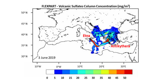
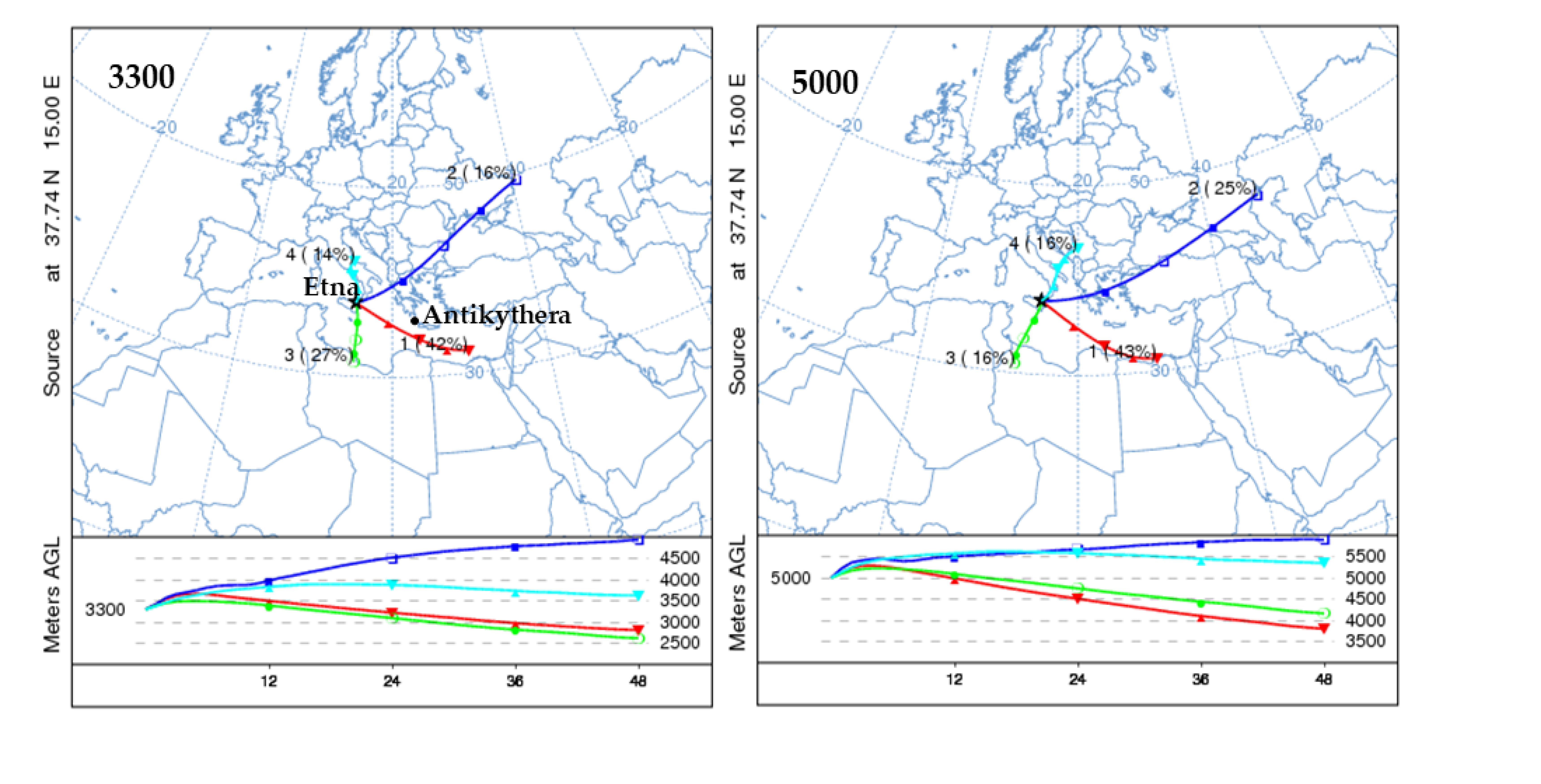
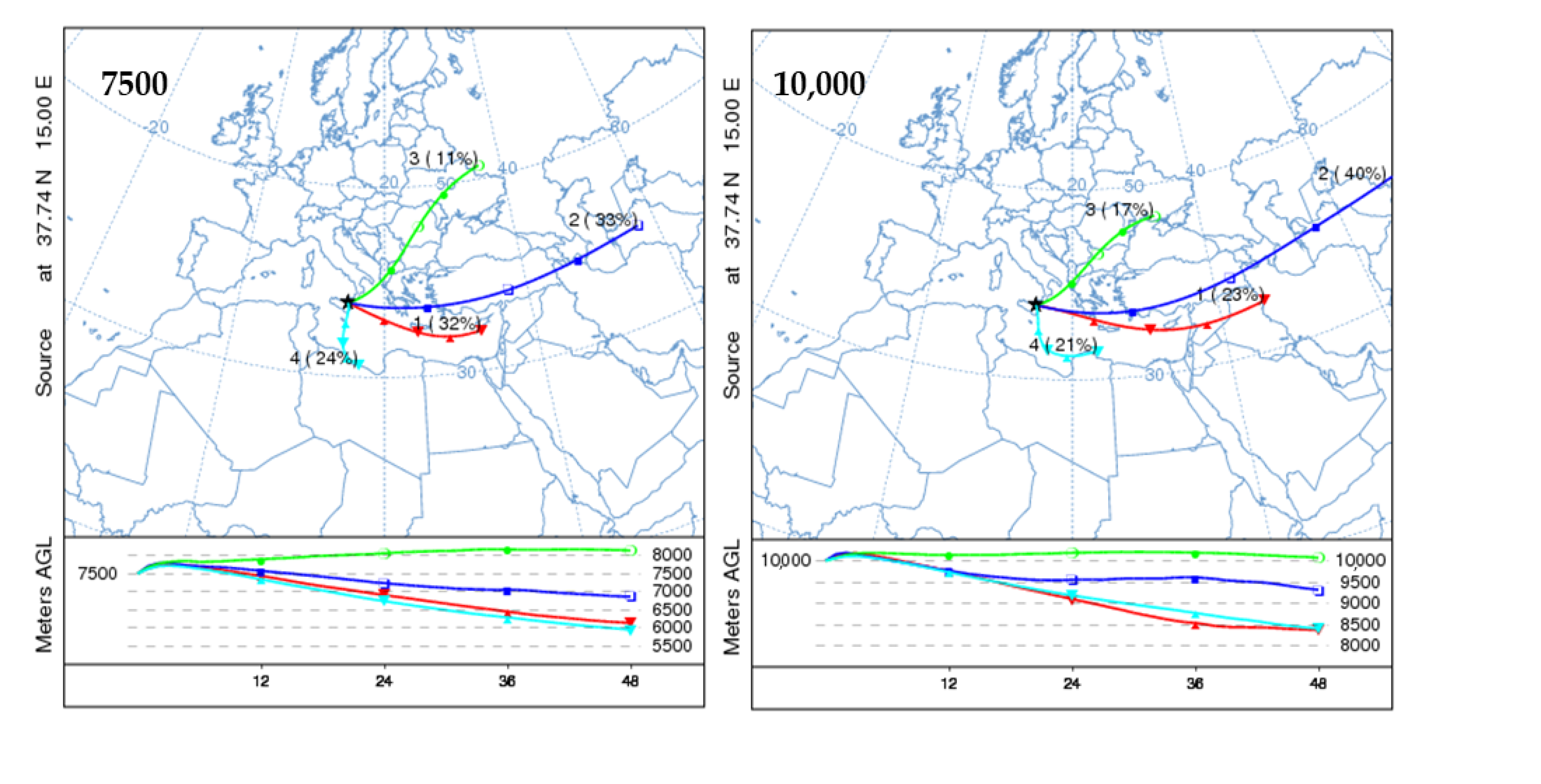
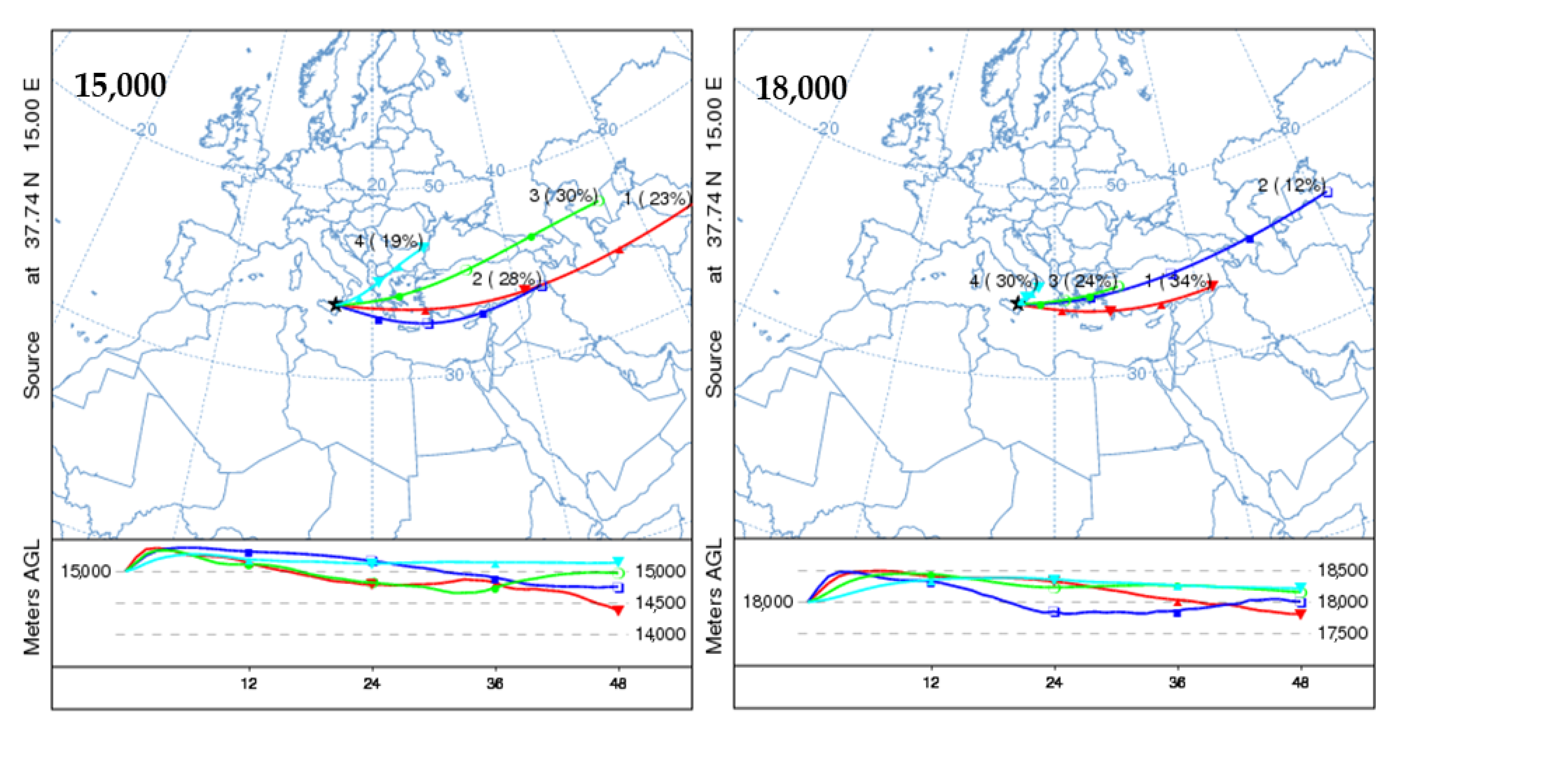
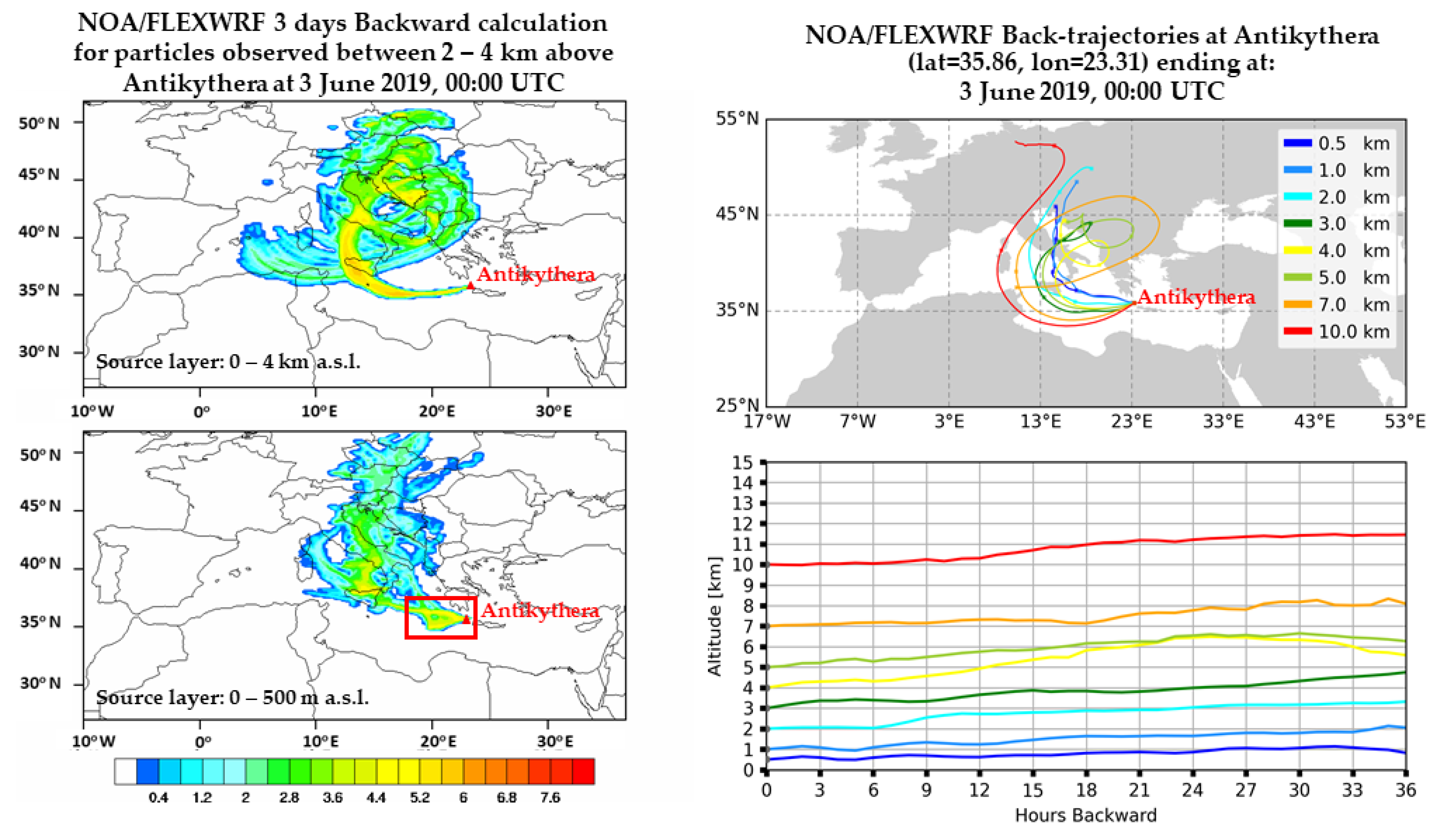
The HYSPLIT cluster analysis indicates that the upper tropospheric—lower stratospheric air masses from Etna are mainly transported eastwards over the Mediterranean and are detected at the new PANGEA observatory of NOA at the island of Antikythera establishing the Etna—Antikythera connection. The PANGEA observatory is located 765 km downwind the volcano and presents an important infrastructure for the monitoring of volcanic emissions from Etna.
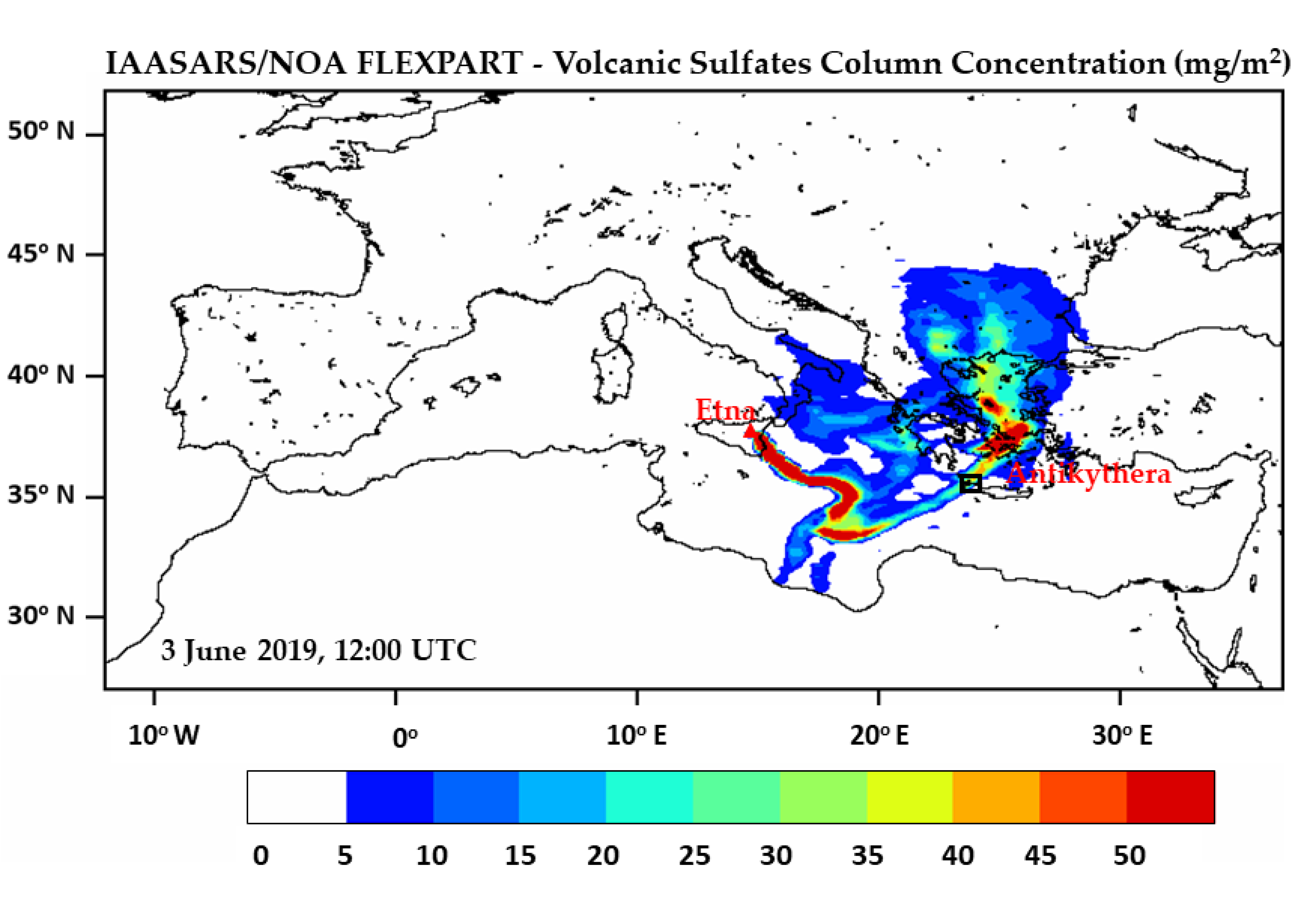
2:
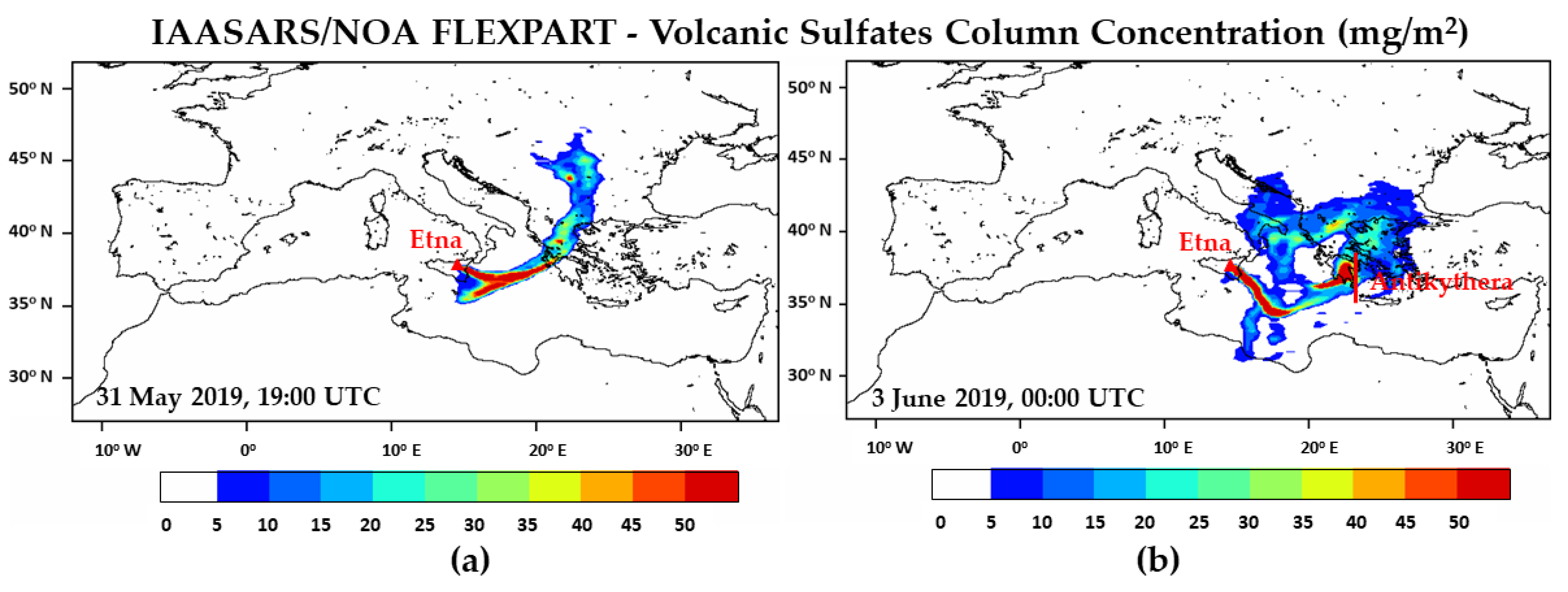
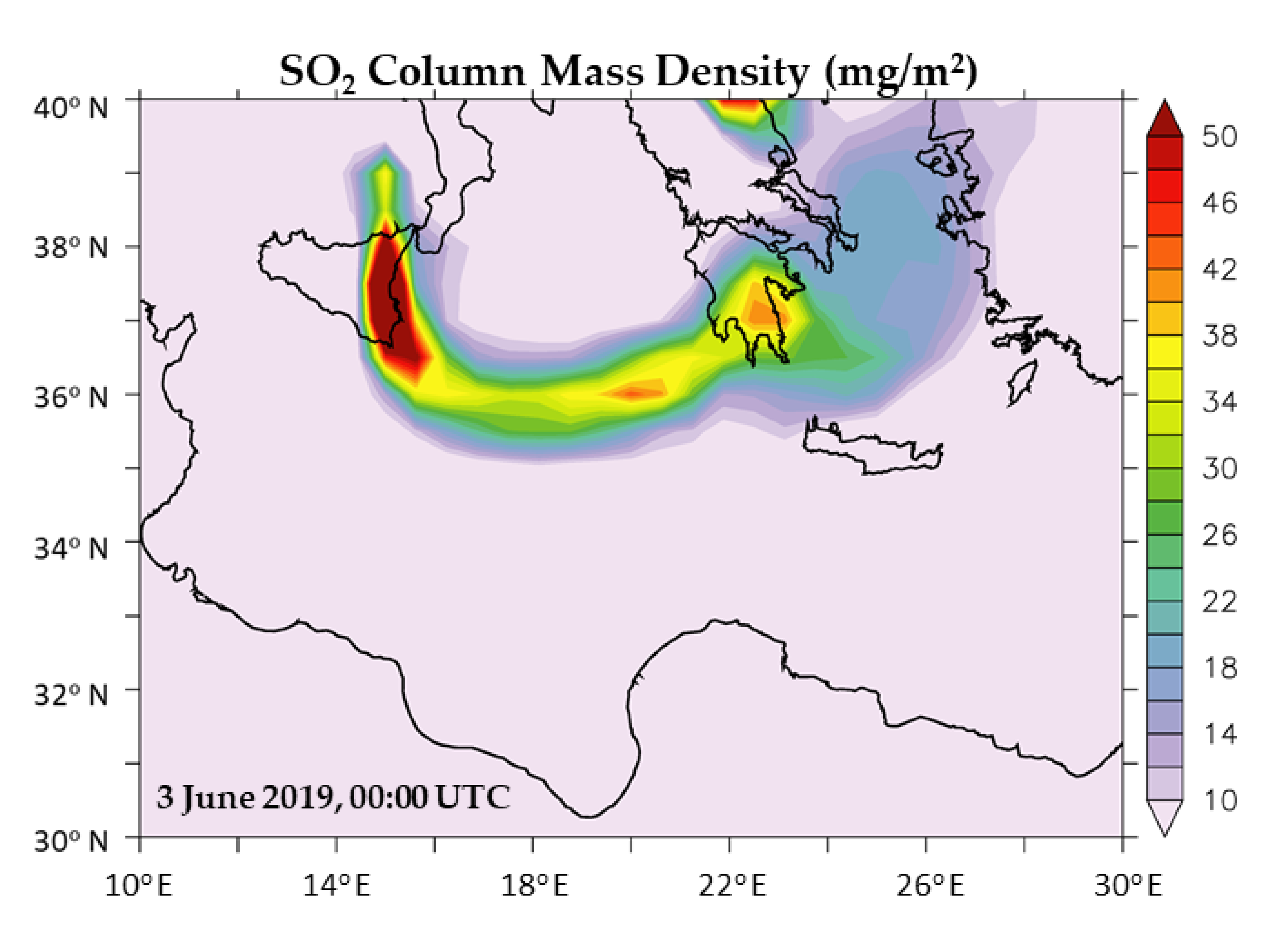
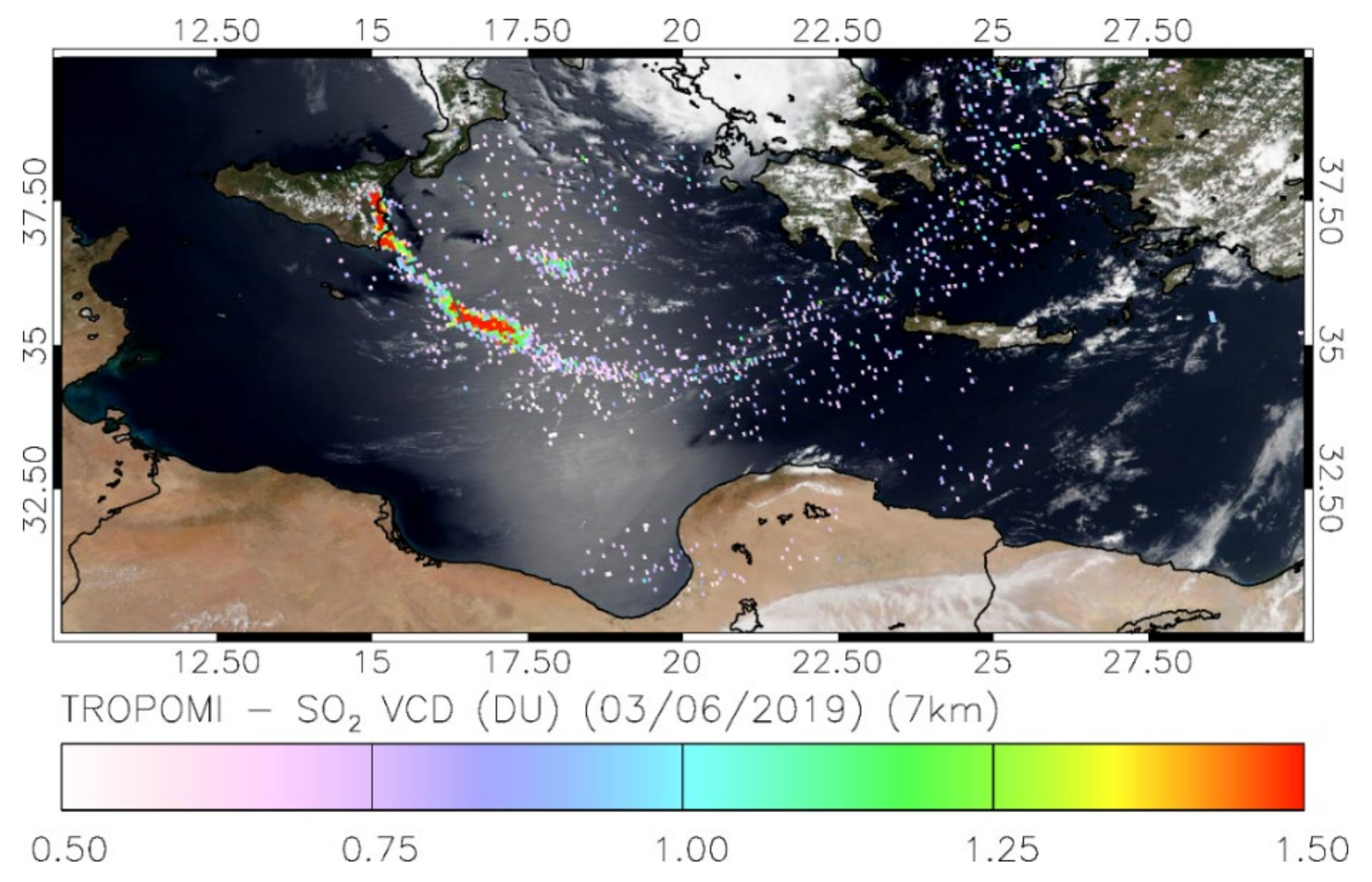
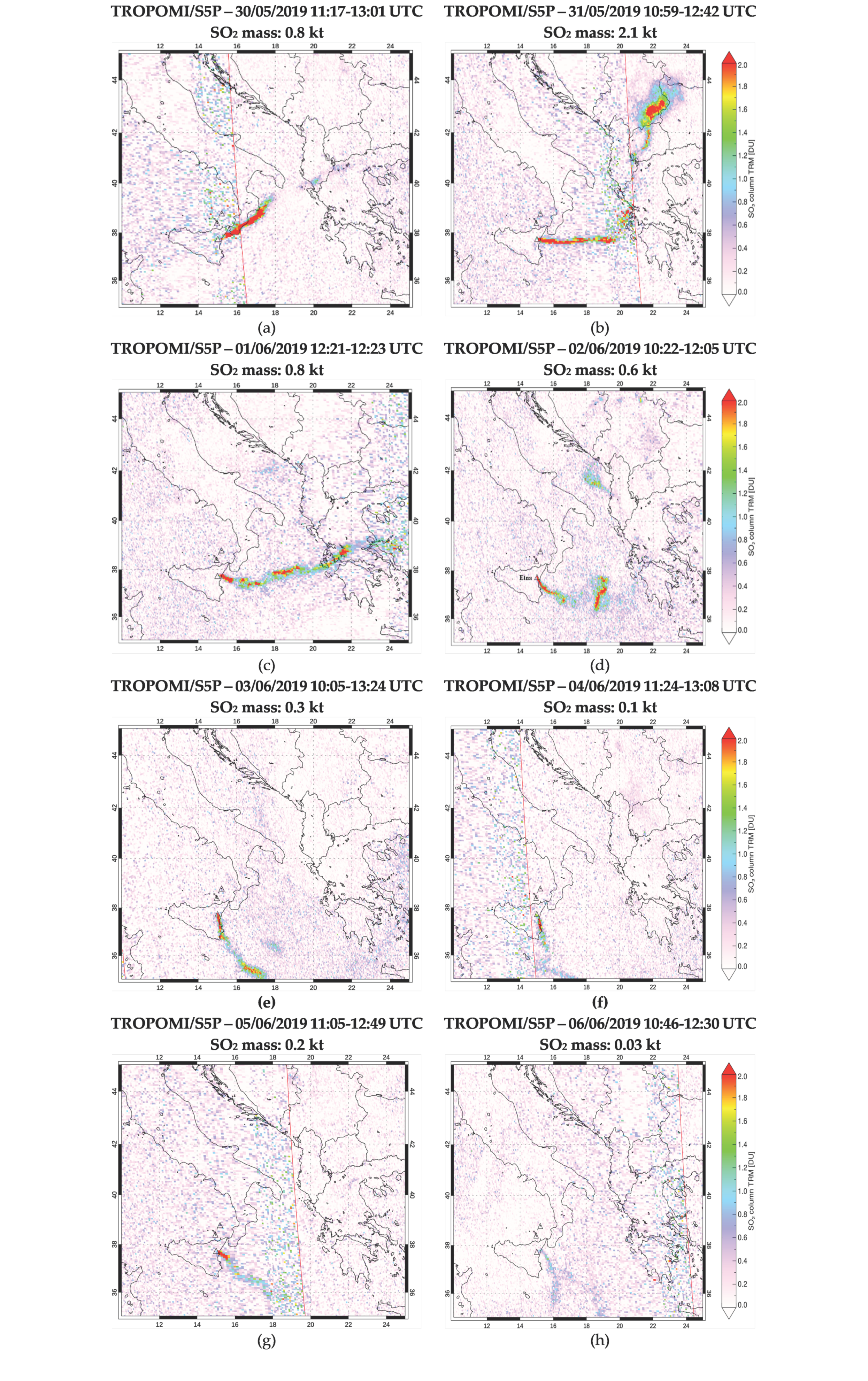
The long-range dispersion of sulfates from Etna was simulated with FLEXPART-WRF using an emission rate of 4 kt/day. The sulfates plume spreads mainly northeastward from the volcano and takes a circular shape due to a passing cyclone, while on 3 June 2019, the plume has covered the northeastern parts of Greece, with the main part shifting towards the southern parts of the country and reaching the Antikythera station. This is consistent with the observed movement of the simulated sulfates plume as depicted from TROPOMI, as well as with the MERRA-2 reanalysis products.
3:
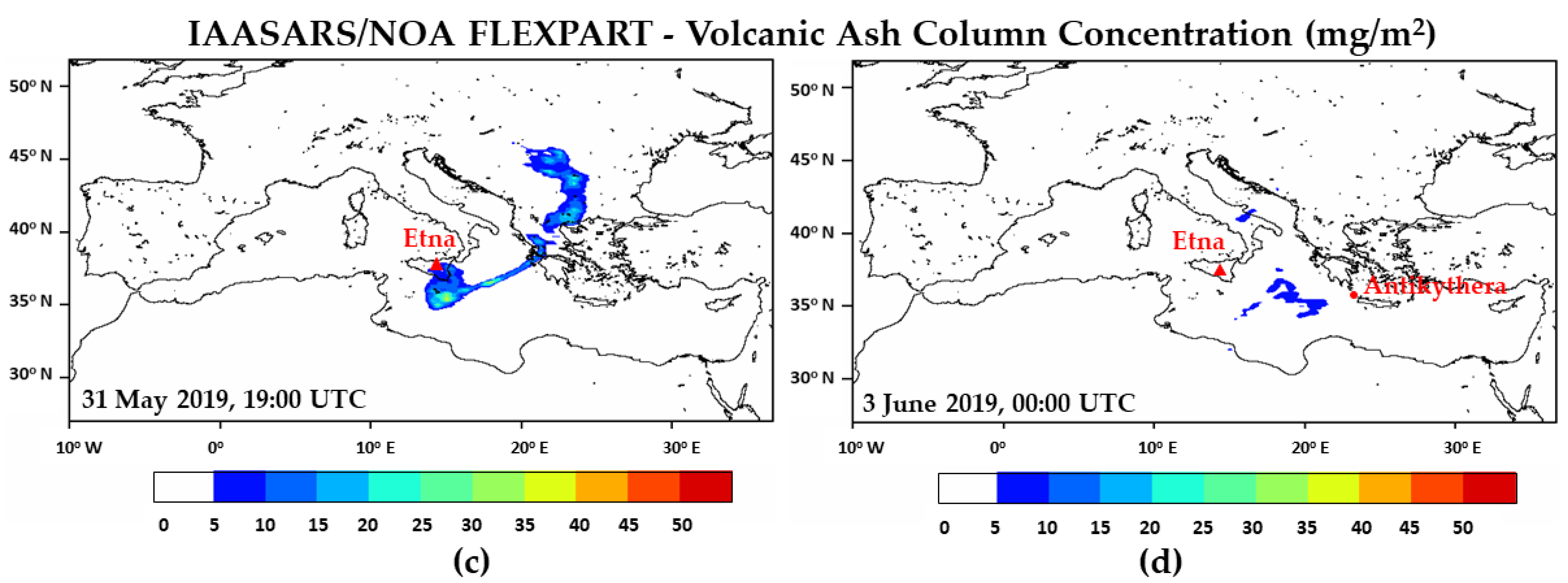
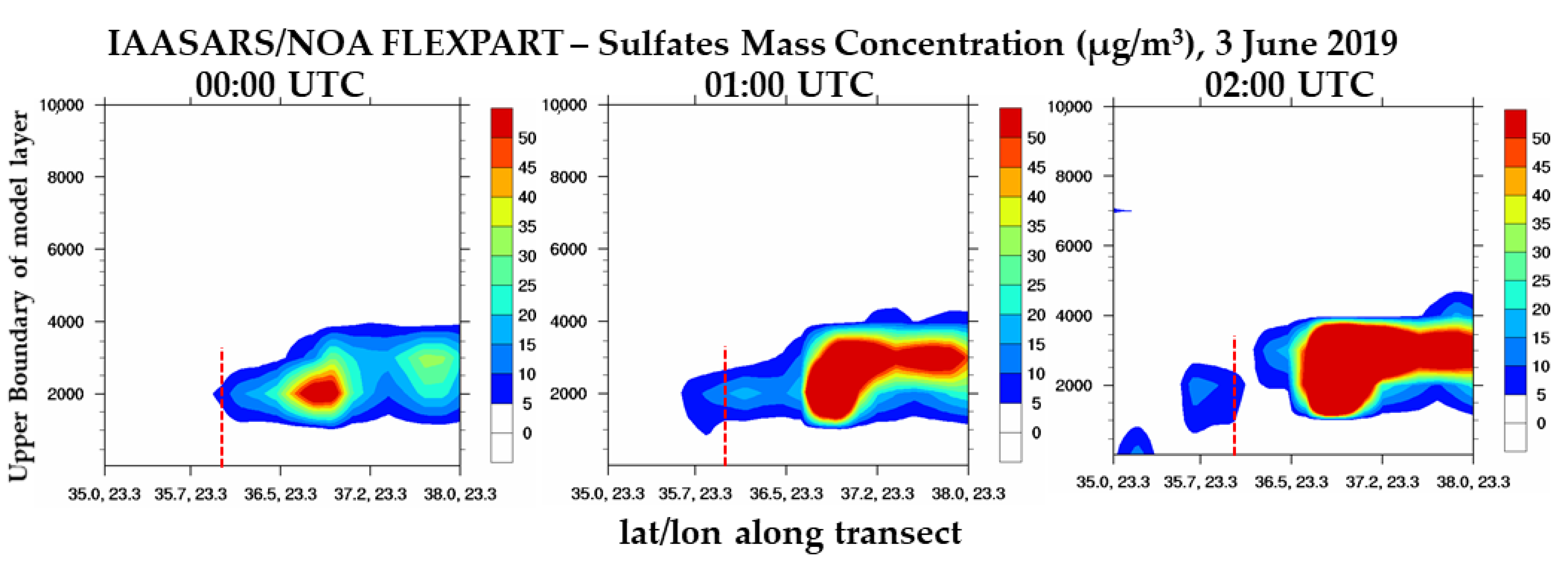
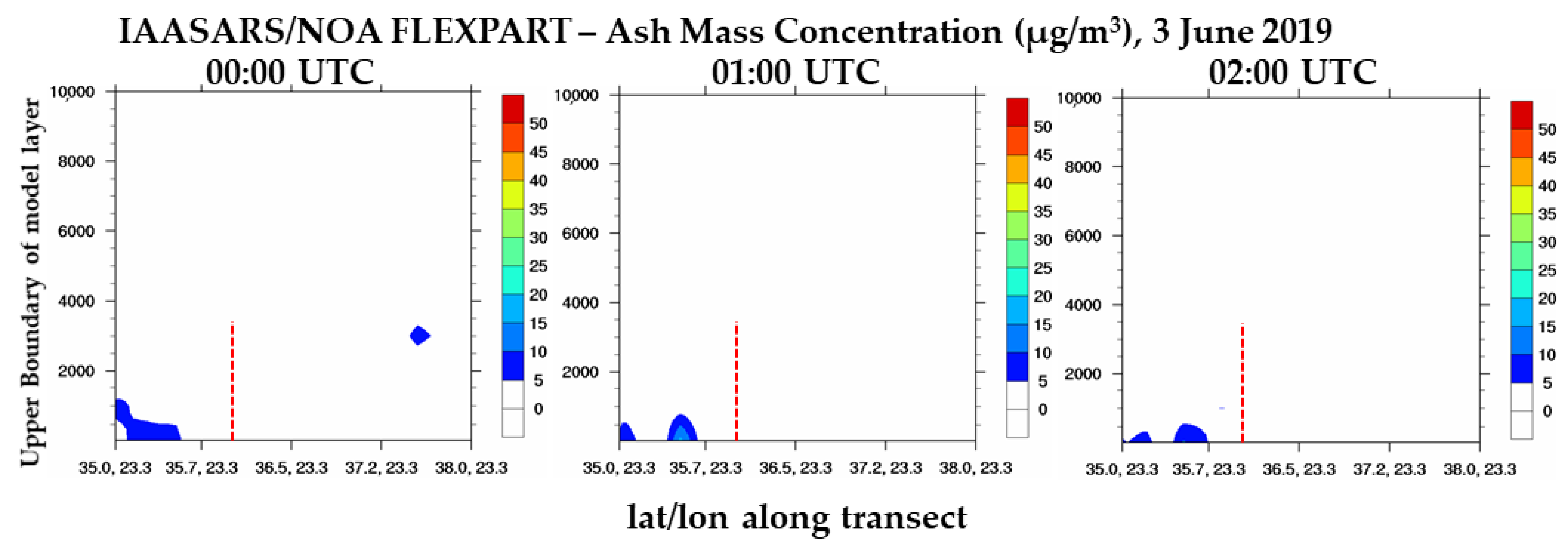
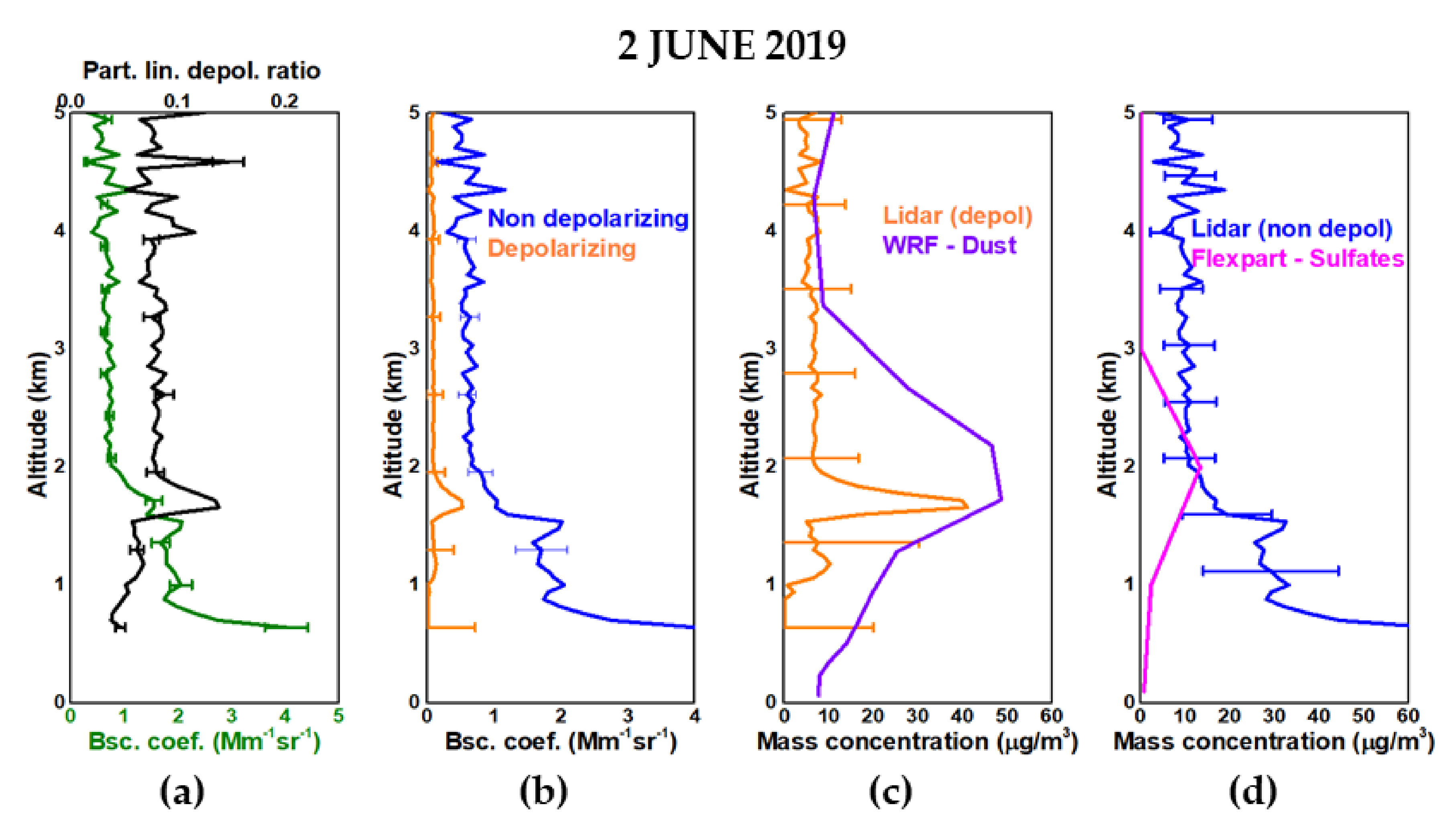
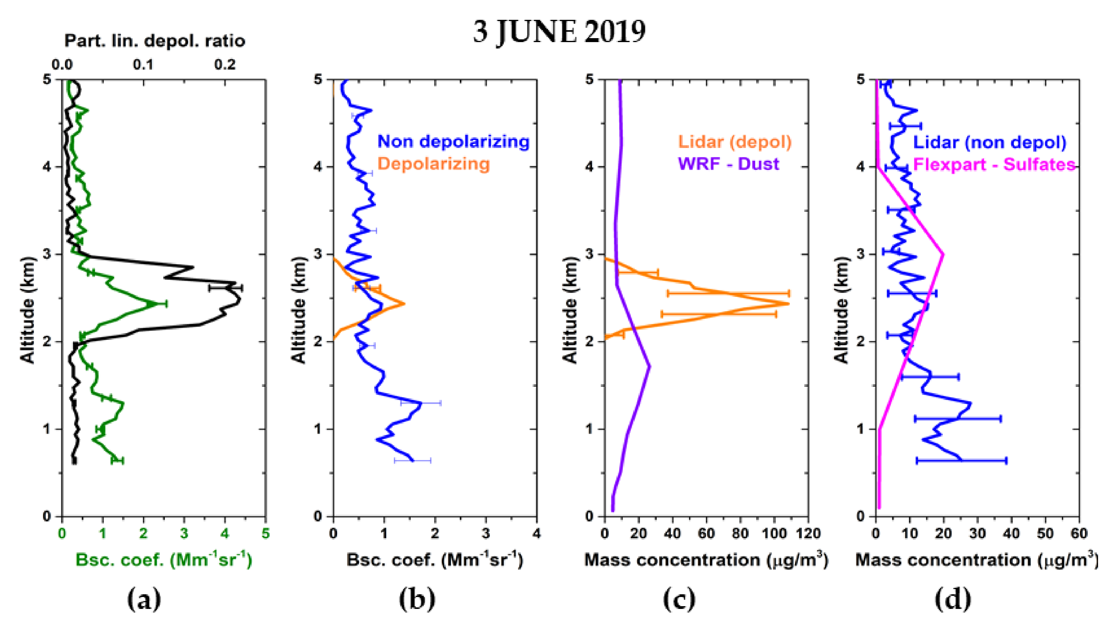
FLEXPART-WRF simulations for volcanic ash were performed with mass values of the order of 105 kg/s following the studies of weak plumes with wind conditions [23,64]. The transport and the different followed paths of sulfates and volcanic ash driven by FLEXPART-WRF show that both plumes move eastward but only sulfate plumes reach the southern parts of Greece. The modeled sulfate mass concentration is approximately 18 μg/m3 for the first plume and 20 μg/m3 for the second plume on 2 and 3 June 2019, respectively, whereas the ash mass concentration is below 5 μg/m3 on 3 June 2019, at 18:00 UTC.
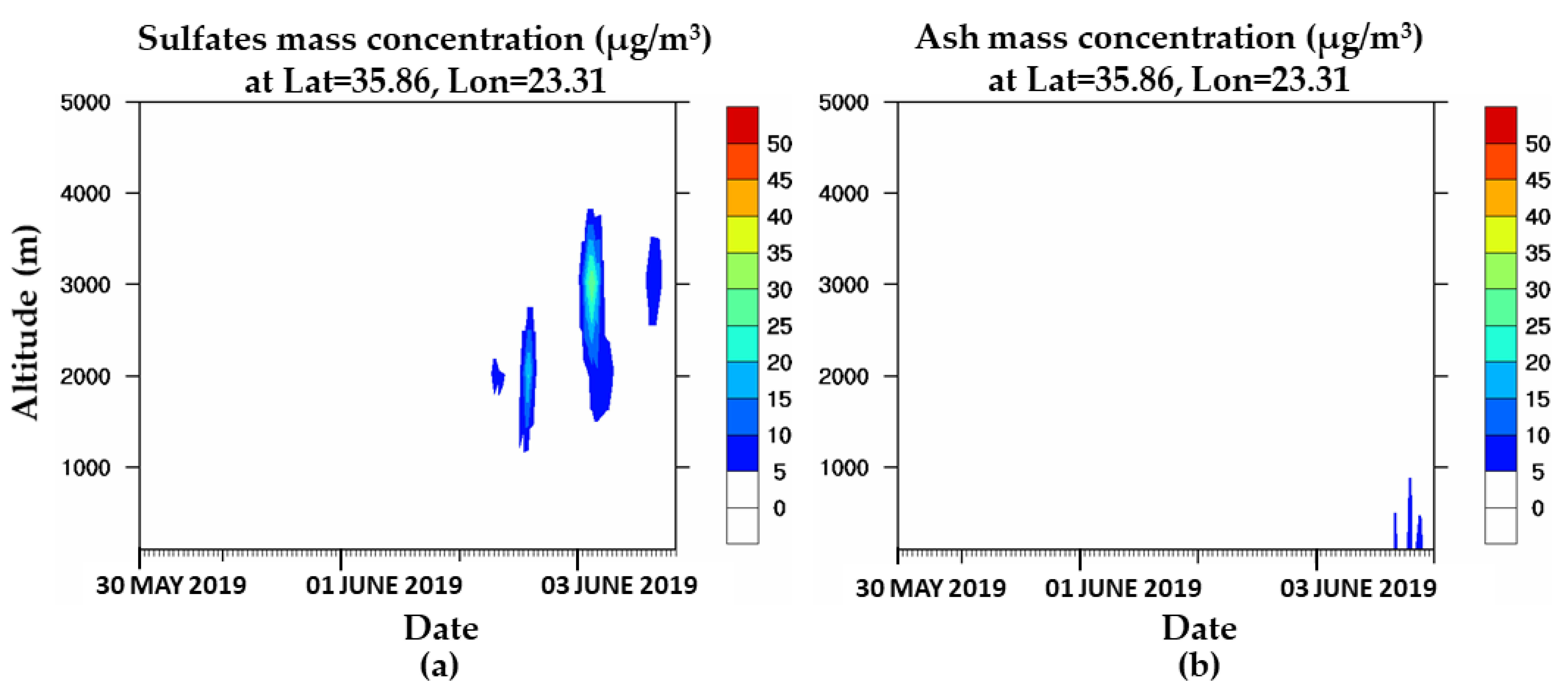
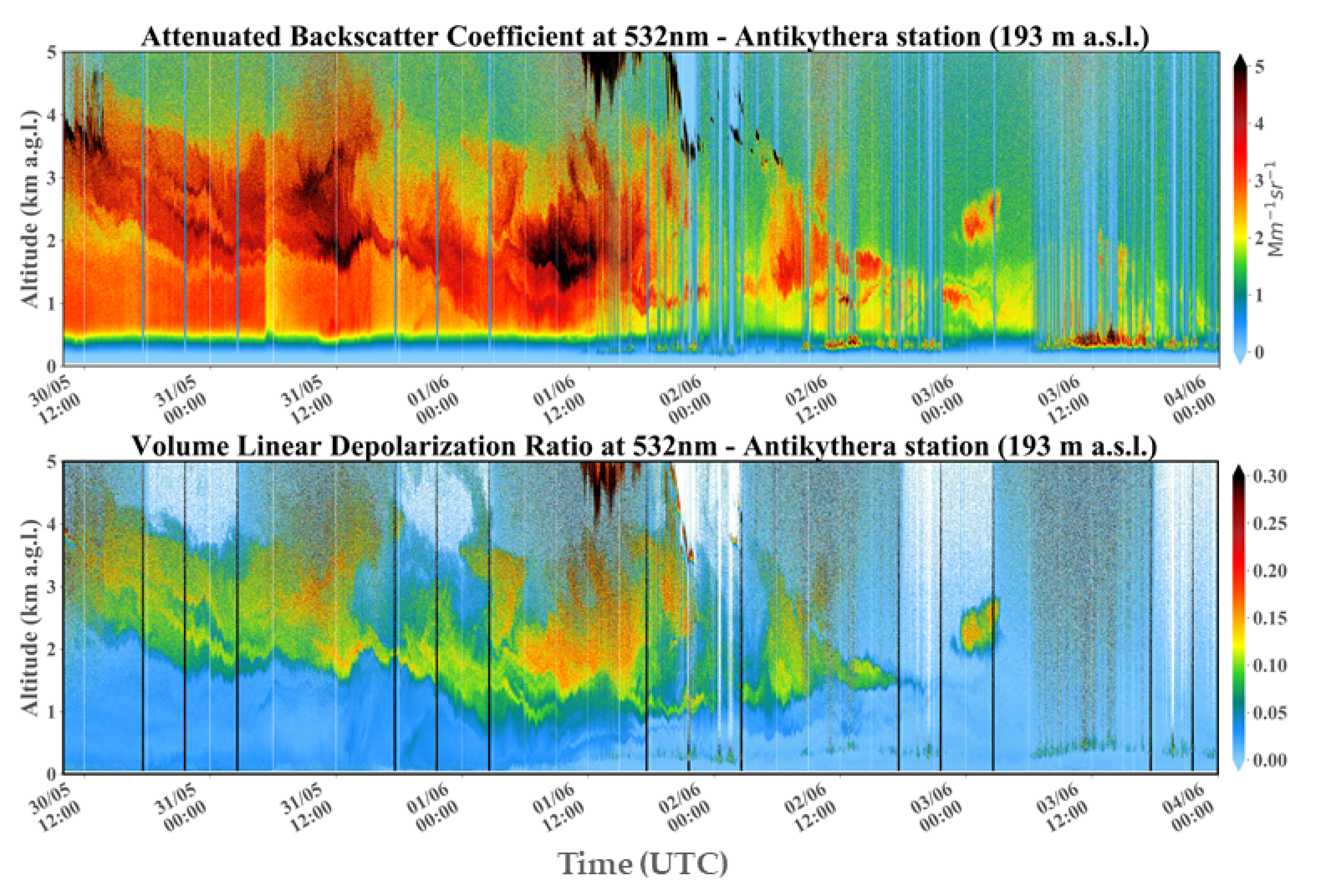
4:
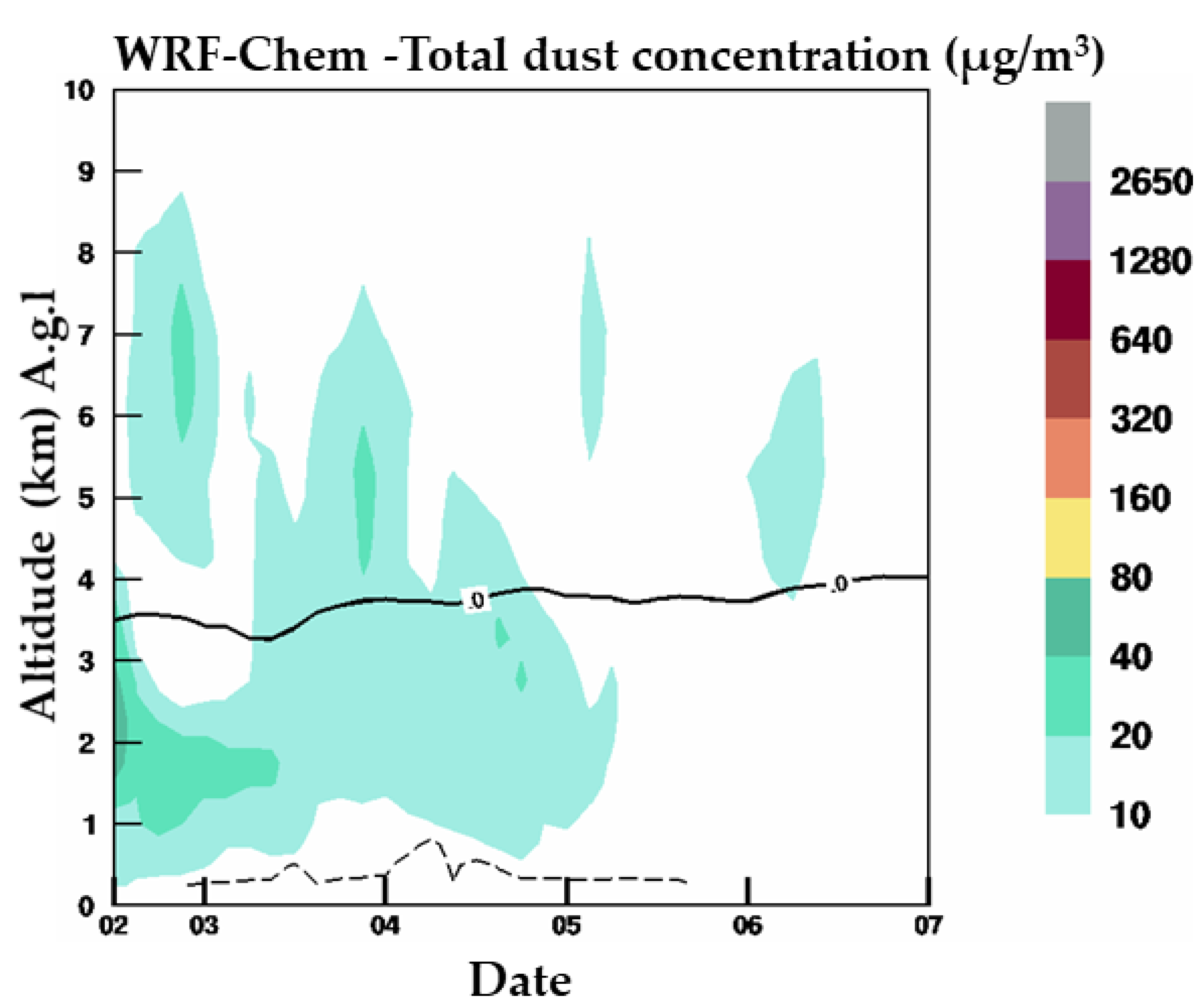
The height and mass concentration of the simulated two sulfate plumes were evaluated in a qualitative manner using PANGEA measurements. According to the PollyXT-NOA observations, the two elevated plumes are located between 1 and 2 km and 2 and 3 km above the local PBL on 2 June 2019, 17:00–18:00 UTC and 3 June 2019, 00:00–02:00 UTC respectively, three and four days after the eruption. For this time windows, the possible contribution of ash and sulfate particles to the lidar backscatter coefficient profile β at 532 nm was separated based on the POLIPHON technique. For the sulfates mass concentration, the agreement between the model and the lidar is satisfactory, with the depth of the two sulfate layers to be well captured by the model. On the contrary, the volcanic ash plume is not accurately reproduced by the model for the selected time interval. By comparing the modeled ash and dust mass concentrations to lidar profiles the agreement with the lidar is more satisfactory for dust particles.
5:
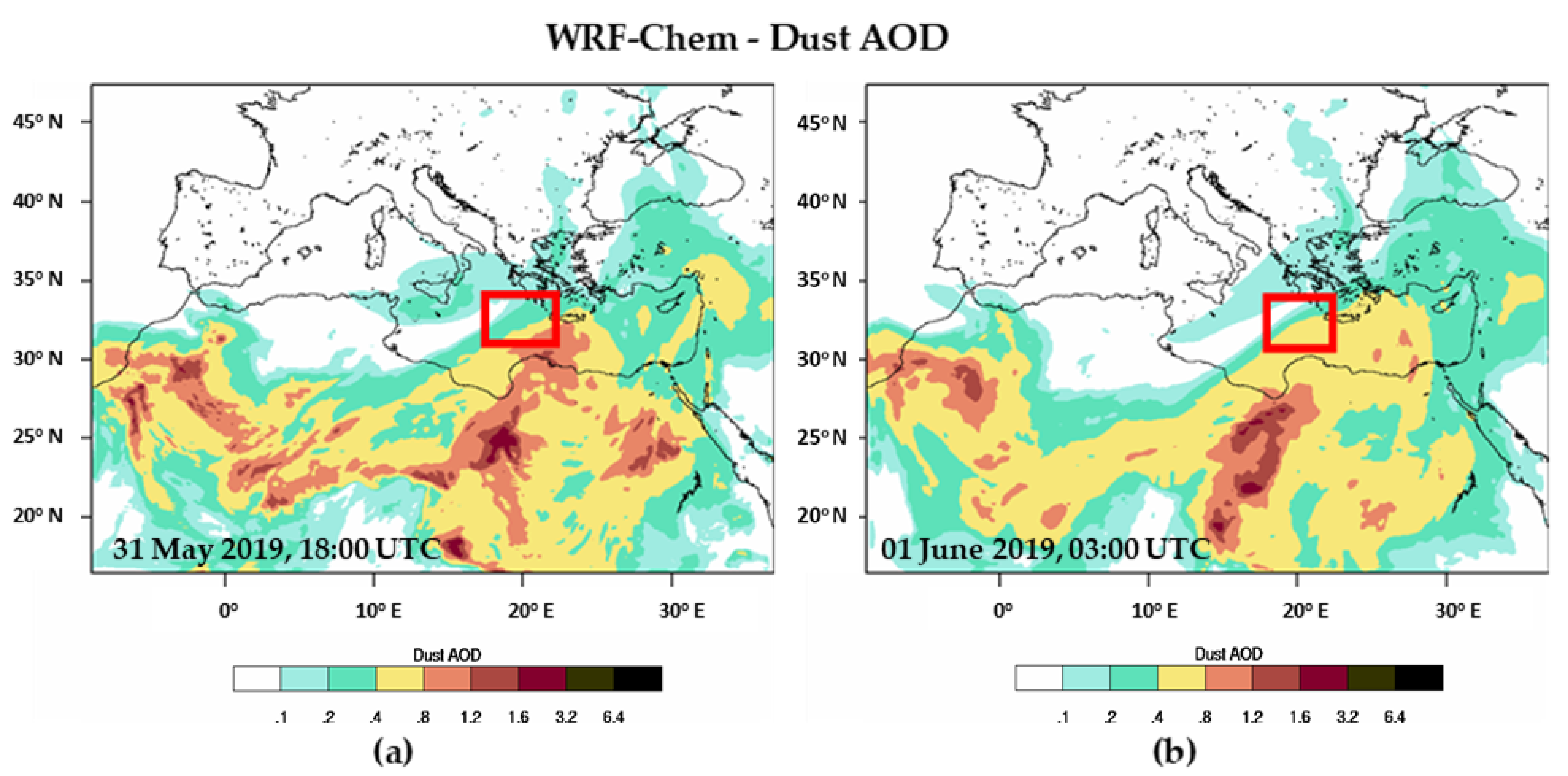
Finally, the combined information of the backward trajectory analysis, the source-receptor relationships and the results of the WRF-Chem model at Antikythera station, on 3 June 2019, at 00:00 UTC indicate the presence of a mixture of volcanic sulfates and dust particles.
The above complex interactions between different aerosol and gas species and the meteorological patterns of the Mediterranean indicate the need to intensify the relevant research activities in this area. As an important step in this direction, the development of PANGEA observatory in Antikythera offers the chance for continuous monitoring of atmospheric tracers. As shown in this study, volcanic ash and sulfate particles may coexist with dust, marine, biogenic, and anthropogenic aerosols over the Mediterranean. This gives us the opportunity to extend our future research by applying also quantitative inversion algorithms (e.g., [96]) to largely improve the predictions of volcanic ash fluxes from Etna eruptions and also the separation between different species constrained by ground-based and satellite measurement data.

Author Contributions

Conceptualization, A.K., V.A., S.S. (Stavros Solomos) and A.G.; Data curation, A.K., S.S. (Simona Scollo), M.T. and I.T.; Investigation, A.K.; Methodology, A.K., V.A., S.S. (Stavros Solomos), A.G., E.M., C.S., A.K.G., D.A., N.P. and P.Z.; Software, A.K., E.M., C.S. and A.K.G.; Supervision, C.S., V.A., S.S. (Stavros Solomos) and P.Z.; Visualization, A.K., A.G. and E.M.; Writing – original draft, A.K., V.A., S.S. (Stavros Solomos), A.G. and P.Z.; Writing – review & editing, V.A., S.S. (Stavros Solomos), E.M., C.S., A.K.G., D.A., N.P., L.M., S.S. (Simona Scollo), I.P., T.K. and P.Z. All authors have read and agreed to the published version of the manuscript.

Funding

This research was funded by EU H2020 E-shape project (Grant Agreement n. 820852) and by the project “PANhellenic infrastructure for Atmospheric Composition and climatE change” (MIS 5021516) which is implemented under the Action “Reinforcement of the Research and Innovation Infrastructure”, funded by the Operational Programme “Competitiveness, Entrepreneurship and Innovation” (NSRF 2014–2020) and co-financed by Greece and the European Union (European Regional Development Fund)”. This research was also funded by “Stavros Niarchos Foundation (SNF)”.

Data Availability statement

The satellite products used in this study are the VIIRS/Suomi-NPP imagery which is publicly available from NASA Worldview application (https://worldview.earthdata.nasa.gov); the TROPOMI/S5P imagery publicly available from NASA’s Global Sulfur Dioxide Monitoring Home Page (https://so2.gsfc.nasa.gov/); the TROPOMI/S5P data are publicly available via the Copernicus S5P hub (https://scihub.copernicus.eu/). The MERRA-2 data are publicly available via NASA GMAO (https://disc.gsfc.nasa.gov/datasets/M2T1NXAER_5.12.4/summary). The PollyXT observations (level 0 data of measured signals and level 2 data of backscatter coefficient and depolarization profiles) and the derived POLIPHON profiles and concentrations used in this study can be accessed through the REACT database (Kampouri et al., 2020). The FLEXPART-WRF model data are available from the corresponding author (A.K.) upon request. Kampouri, A.; Amiridis, V.; Solomos, S.; Gialitaki, A.; Marinou, E.; Spyrou, C.; Georgoulias, A.K.; Akritidis, D.; Papagiannopoulos, N.; Mona, L.; Scollo, S.; Tsichla, M.; Tsikoudi, I.; Pytharoulis, I.; Karacostas, T.; Zanis, P.: available at: https://react.space.noa.gr/papers/Kampouri_et_al_2020/Dataset, last access: 05 January 2021.

Acknowledgments

The authors acknowledge EARLINET for providing aerosol lidar profiles (https://www.earlinet.org). We thank the ACTRIS-2 and ACTRIS preparatory phase projects that have received funding from the European Union’s Horizon 2020 Framework Program for Research and Innovation (grant agreement no. 654109) and from European Union’s Horizon 2020 Coordination and Support Action (grant agreement no. 739530), respectively. This research was also supported by the European Research Council (ERC) under the European Community’s Horizon 2020 research and innovation framework programme—ERC grant agreement no. 725698 (D-TECT). We acknowledge the support by EU H2020 E-shape project (Grant Agreement n. 820852). Video-surveillance system of Etna is operated by INGV-OE and we thank all technicians and technologists involved in their maintenance. Eleni Marinou was funded by a DLR VO-Ryoung investigator group and the Deutscher Akademischer Austauschdienst (grant no. 57370121). This research was also supported by data and services obtained from the PANhellenic Geophysical Observatory of Antikythera (PANGEA) of the National Observatory of Athens (NOA), Greece and by the project “PANhellenic infrastructure for Atmospheric Composition and climatE change” (MIS 5021516) which is implemented under the Action “Reinforcement of the Research and Innovation Infrastructure”, funded by the Operational Programme “Competitiveness, Entrepreneurship and Innovation” (NSRF 2014-2020) and co-financed by Greece and the European Union (European Regional Development Fund). NOA team acknowledges the support of Stavros Niarchos Foundation (SNF). The authors acknowledge the use of imagery from the NASA Worldview application (https://worldview.earthdata.nasa.gov), part of the NASA Earth Observing System Data and Information System (EOSDIS) and NASA’s Global Sulfur Dioxide Monitoring Home Page (https://so2.gsfc.nasa.gov/) and the use of modified Copernicus Sentinel data 2019. Finally, the MERRA-2 community is acknowledged for producing and distributing the reanalysis data used in the present work.

Conflicts of Interest

The authors declare no conflict of interest.

Appendix A

Figure A1. SO2 mass burden collected by TROPOMI/S5P, data from: BIRA-IASB/DLR/ESA/EU Copernicus Program. The SO2 mass burden varies over Etna from day to day: (a) on 30 May 2019, 11:17–13:01 UTC, (b) on 31 May 2019, 10:59–12:42 UTC, (c) on 1 June 2019, 12:21–12:23 UTC, (d) on 2 June 2019, 10:22–12:05 UTC, (e) on 3 June 2019, 10:05–13:24 UTC, (f) on 4 June 2019, 11:24–13:08 UTC, (g) on 5 June 2019, 11:05–12:49 UTC, and (h) on 6 June 2019, 10:46–12:30 UTC (https://so2.gsfc.nasa.gov/).
Atmosphere 12 00040 g0a1
Figure A2. (a) Modeled dust AOD (in μg/m3) on 31 May 2019 18:00 UTC and (b) on 1 June 2019, 03:00 UTC. The location of the possible dust-prone areas above Mediterranean Sea is marked with a red square.
Atmosphere 12 00040 g0a2
Figure A3. Simulated column concentration of sulfate particles (mg/m2) originating from Etna, on 3 June 2019, 12:00 UTC, as simulated by FLEXPART-WRF using the SO2 source term. The location of the Etna Volcano is marked with a red triangle and with black square the Antikythera Island.
Atmosphere 12 00040 g0a3

References

  1. Textor, C.; Graf, H.F.; Herzog, M.; Oberhuber, J.M. Injection of gases into the stratosphere by explosive volcanic eruptions. J. Geophys. Res. Atmos. 2003, 108, 4606. [Google Scholar] [CrossRef] [Green Version]
  2. Robock, A. Climatic impact of volcanic emissions. Geophys. Monogr. Ser. 2004, 150, 125–134. [Google Scholar] [CrossRef] [Green Version]
  3. Stohl, A.; Forster, C.; Frank, A.; Seibert, P.; Wotawa, G. Technical note: The Lagrangian particle dispersion model FLEXPART version 6.2. Atmos. Chem. Phys. 2005, 5, 2461–2474. [Google Scholar] [CrossRef] [Green Version]
  4. Kristiansen, N.I.; Stohl, A.; Prata, A.J.; Bukowiecki, N.; Dacre, H.; Eckhardt, S.; Henne, S.; Hort, M.C.; Johnson, B.T.; Marenco, F.; et al. Performance assessment of a volcanic ash transport model mini-ensemble used for inverse modeling of the 2010 Eyjafjallajkull eruption. J. Geophys. Res. Atmos. 2012, 117, D20. [Google Scholar] [CrossRef] [Green Version]
  5. Roberts, T.; Dayma, G.; Oppenheimer, C. Reaction rates control high-temperature chemistry of volcanic gases in air. Front. Earth Sci. 2019, 7. [Google Scholar] [CrossRef] [Green Version]
  6. Mather, T.A.; Pyle, D.M.; Oppenheimer, C. Troposheric volcanic aerosol. Geophys. Monogr. 2003, 139, 189–212. [Google Scholar]
  7. Hobbs, P.V. Introduction to Atmospheric Chemistry; Cambridge University Press: Cambridge, UK, 2000. [Google Scholar]
  8. Andres, R.J.; Kasgnoc, A.D. A time-averaged inventory of subaerial volcanic sulfur emissions. J. Geophys. Res. Atmos. 1998, 103, 25251–25261. [Google Scholar] [CrossRef]
  9. Carn, S.A.; Fioletov, V.E.; Mclinden, C.A.; Li, C.; Krotkov, N.A. A decade of global volcanic SO2 emissions measured from space. Sci. Rep. 2017, 7, 44095. [Google Scholar] [CrossRef] [PubMed] [Green Version]
  10. Stevenson, D.S.; Johnson, C.E.; Collins, W.J.; Derwent, R.G. The Tropospheric Sulphur Cycle and the Role of Volcanic SO2; The Geological Society of London: London, UK, 2003; Volume 213. [Google Scholar]
  11. Graf, H.F.; Langmann, B.; Feichter, J. The contribution of Earth degassing to the atmospheric sulfur budget. Chem. Geol. 1998, 147, 131–145. [Google Scholar] [CrossRef]
  12. Galeazzo, T.; Bekki, S.; Martin, E.; Savarino, J.A.; Arnold, R.; Galeazzo, T.; Bekki, S.; Martin, E.; Savarino, J.A.; Photo, S.R.A.; et al. Photochemical box modelling of volcanic SO2 oxidation: Isotopic constraints to cite this version: HAL Id: Insu-01966512 Photochemical box modelling of volcanic SO2 oxidation: Isotopic constraints. Atmos. Chem. Phys. 2018. [Google Scholar] [CrossRef] [Green Version]
  13. Solomon, S.; Portmann, R.W.; Garcia, R.R.; Randel, W.; Wu, F.; Nagatani, R.; Gleason, L.; Thomason, L.; Poole, L.R.; McCormick, M.P. Ozone depletion at mid-latitudes: Coupling of volcanic aerosols and temperature variability to anthropogenic chlorine. Geophys. Res. Lett. 1998, 25, 1871–1874. [Google Scholar] [CrossRef]
  14. Blake, D.M.; Wilson, T.M.; Gomez, C. Road marking coverage by volcanic ash: An experimental approach. Environ. Earth Sci. 2016, 75, 1348. [Google Scholar] [CrossRef]
  15. Sellitto, P.; Briole, P. On the radiative forcing of volcanic plumes: Modelling the impact of Mount Etna in the Mediterranean. Ann. Geophys. 2015, 58. [Google Scholar] [CrossRef]
  16. Sellitto, P.; Di Sarra, A.; Corradini, S.; Boichu, M.; Herbin, H.; Dubuisson, P.; Sèze, G.; Meloni, D.; Monteleone, F.; Merucci, L.; et al. Synergistic use of Lagrangian dispersion and radiative transfer modelling with satellite and surface remote sensing measurements for the investigation of volcanic plumes: The Mount Etna eruption of 25-27 October 2013. Atmos. Chem. Phys. 2016, 16, 6841–6861. [Google Scholar] [CrossRef] [Green Version]
  17. Timmreck, C.; Toohey, M.; Stenke, A.; Schwarz, J.P.; Weigel, R. Reviews of Geophysics and impact on climate. Rev. Geophys. 2016, 54, 278–335. [Google Scholar] [CrossRef]
  18. Akritidis, D.; Katragkou, E.; Georgoulias, A.K.; Zanis, P.; Kartsios, S.; Flemming, J.; Inness, A.; Douros, J.; Eskes, H. A complex aerosol transport event over Europe during the 2017 Storm Ophelia in CAMS forecast systems: Analysis and evaluation. Atmos. Chem. Phys. 2020, 20, 13557–13578. [Google Scholar] [CrossRef]
  19. Schneider, D.J.; Dean, K.G.; Dehn, J.; Miller, T.P.; Kirianov, V.Y. Monitoring and Analyses of Volcanic Activity Using Remote Sensing Data at the Alaska Volcano Observatory: Case Study for Kamchatka, Russia, December 1997; American Geophysical Union: Washington, DC, USA, 2000; Volume 116, ISBN 9781118664513. [Google Scholar]
  20. Prata, A.J.; Tupper, A. Aviation hazards from volcanoes: The state of the science. Nat. Hazards 2009, 51, 239–244. [Google Scholar] [CrossRef] [Green Version]
  21. Zerefos, C.S.; Eleftheratos, K.; Kapsomenakis, J.; Solomos, S.; Inness, A.; Balis, D.; Redondas, A.; Eskes, H.; Allaart, M.; Amiridis, V.; et al. Detecting volcanic sulfur dioxide plumes in the Northern Hemisphere using the Brewer spectrophotometers, other networks, and satellite observations. Atmos. Chem. Phys. 2017, 17, 551–574. [Google Scholar] [CrossRef] [Green Version]
  22. Moxnes, E.D. Estimating the Sulphur Dioxide and Ash Emissions from the Grímsvötn 2011 Volcanic Eruption and Simulating Their Transport across Northern Europe. Master’s Thesis, University of Oslo, Oslo, Norway, 2011. [Google Scholar]
  23. Scollo, S.; Prestifilippo, M.; Bonadonna, C.; Cioni, R.; Corradini, S.; Degruyter, W.; Rossi, E.; Silvestri, M.; Biale, E.; Carparelli, G.; et al. Near-real-time tephra fallout assessment at Mt. Etna, Italy. Remote Sens. 2019, 11, 2987. [Google Scholar] [CrossRef] [Green Version]
  24. Hughes, E.J.; Yorks, J.; Krotkov, N.A.; da Silva, A.M.; McGill, M. Using CATS near-real-time lidar observations to monitor and constrain volcanic sulfur dioxide (SO2) forecasts. Geophys. Res. Lett. 2016, 43, 11089–11097. [Google Scholar] [CrossRef]
  25. Papagiannopoulos, N.; D’Amico, G.; Gialitaki, A.; Ajtai, N.; Alados-Arboledas, L.; Amodeo, A.; Amiridis, V.; Baars, H.; Balis, D.; Binietoglou, I.; et al. An EARLINET early warning system for atmospheric aerosol aviation hazards. Atmos. Chem. Phys. 2020, 20, 10775–10789. [Google Scholar] [CrossRef]
  26. Veefkind, J.P.; Aben, I.; McMullan, K.; Förster, H.; de Vries, J.; Otter, G.; Claas, J.; Eskes, H.J.; de Haan, J.F.; Kleipool, Q.; et al. TROPOMI on the ESA Sentinel-5 Precursor: A GMES mission for global observations of the atmospheric composition for climate, air quality and ozone layer applications. Remote Sens. Environ. 2012, 120, 70–83. [Google Scholar] [CrossRef]
  27. Queißer, M.; Burton, M.; Theys, N.; Pardini, F.; Salerno, G.; Caltabiano, T.; Varnam, M.; Esse, B.; Kazahaya, R. TROPOMI enables high resolution SO2 flux observations from Mt. Etna, Italy, and beyond. Sci. Rep. 2019, 9, 957. [Google Scholar] [CrossRef] [PubMed]
  28. Sassen, K.; Zhu, J.; Webley, P.; Dean, K.; Cobb, P. Volcanic ash plume identification using polarization lidar: Augustine eruption, Alaska. Geophys. Res. Lett. 2007, 34, 5–8. [Google Scholar] [CrossRef]
  29. Wiegner, M.; Gasteiger, J.; Groß, S.; Schnell, F.; Freudenthaler, V.; Forkel, R. Characterization of the Eyjafjallajökull ash-plume: Potential of lidar remote sensing. Phys. Chem. Earth 2012, 45–46, 79–86. [Google Scholar] [CrossRef]
  30. Vernier, J.P.; Fairlie, T.D.; Murray, J.J.; Tupper, A.; Trepte, C.; Winker, D.; Pelon, J.; Garnier, A.; Jumelet, J.; Pavolonis, M.; et al. An advanced system to monitor the 3D structure of diffuse volcanic ash clouds. J. Appl. Meteorol. Climatol. 2013, 52, 2125–2138. [Google Scholar] [CrossRef]
  31. Papayannis, A.; Mamouri, R.E.; Amiridis, V.; Giannakaki, E.; Veselovskii, I.; Kokkalis, P.; Tsaknakis, G.; Balis, D.; Kristiansen, N.I.; Stohl, A.; et al. Optical properties and vertical extension of aged ash layers over the Eastern Mediterranean as observed by Raman lidars during the Eyjafjallajökull eruption in May 2010. Atmos. Environ. 2012, 48, 56–65. [Google Scholar] [CrossRef]
  32. Thomas, H.E.; Prata, A.J. Sulphur dioxide as a volcanic ash proxy during the April-May 2010 eruption of Eyjafjallajökull Volcano, Iceland. Atmos. Chem. Phys. 2011, 11, 6871–6880. [Google Scholar] [CrossRef] [Green Version]
  33. Scollo, S.; Prestifilippo, M.; Pecora, E.; Corradini, S.; Merucci, L.; Spata, G.; Coltelli, M. Eruption column height estimation of the 2011–2013 Etna lava fountains. Ann. Geophys. 2014, 57. [Google Scholar] [CrossRef] [Green Version]
  34. Mastin, L.G.; Guffanti, M.; Servranckx, R.; Webley, P.; Barsotti, S.; Dean, K.; Durant, A.; Ewert, J.W.; Neri, A.; Rose, W.I.; et al. A multidisciplinary effort to assign realistic source parameters to models of volcanic ash-cloud transport and dispersion during eruptions. J. Volcanol. Geotherm. Res. 2009, 186, 10–21. [Google Scholar] [CrossRef]
  35. Pappalardo, G.; Amodeo, A.; Apituley, A.; Comeron, A.; Freudenthaler, V.; Linné, H.; Ansmann, A.; Bösenberg, J.; D’Amico, G.; Mattis, I.; et al. EARLINET: Towards an advanced sustainable European aerosol lidar network. Atmos. Meas. Tech. 2014, 7, 2389–2409. [Google Scholar] [CrossRef] [Green Version]
  36. Brugnone, F.; D’Alessandro, W.; Calabrese, S.; Vigni, L.L.; Bellomo, S.; Brusca, L.; Prano, V.; Saiano, F.; Parello, F. A christmas gift: Signature of the 24th December 2018 eruption of Mt. Etna on the chemical composition of bulk deposition in eastern sicily. Ital. J. Geosci. 2020, 39, 341–358. [Google Scholar] [CrossRef]
  37. Calabrese, S.; Aiuppa, A.; Allard, P.; Bagnato, E.; Bellomo, S.; Brusca, L.; D’Alessandro, W.; Parello, F. Atmospheric sources and sinks of volcanogenic elements in a basaltic volcano (Etna, Italy). Geochim. Cosmochim. Acta 2011, 75, 7401–7425. [Google Scholar] [CrossRef]
  38. Calabrese, S.; Randazzo, L.; Daskalopoulou, K.; Milazzo, S.; Scaglione, S.; Vizzini, S.; Tramati, C.D.; D’Alessandro, W.; Brusca, L.; Bellomo, S.; et al. Mount Etna volcano (Italy) as a major “dust” point source in the Mediterranean area. Arab. J. Geosci. 2016, 9. [Google Scholar] [CrossRef]
  39. Behncke, B.; Branca, S.; Corsaro, R.A.; De Beni, E.; Miraglia, L.; Proietti, C. The 2011-2012 summit activity of Mount Etna: Birth, growth and products of the new SE crater. J. Volcanol. Geotherm. Res. 2014, 270, 10–21. [Google Scholar] [CrossRef]
  40. Behncke, B.; Fornaciai, A.; Neri, M.; Favalli, M.; Ganci, G.; Mazzarini, F. Lidar surveys reveal eruptive volumes and rates at Etna, 2007-2010. Geophys. Res. Lett. 2016, 43, 4270–4278. [Google Scholar] [CrossRef] [Green Version]
  41. De Beni, E.; Behncke, B.; Branca, S.; Nicolosi, I.; Carluccio, R.; D’Ajello Caracciolo, F.; Chiappini, M. The continuing story of Etna’s New Southeast Crater (2012–2014): Evolution and volume calculations based on field surveys and aerophotogrammetry. J. Volcanol. Geotherm. Res. 2015, 303, 175–186. [Google Scholar] [CrossRef]
  42. Acocella, V.; Neri, M.; Behncke, B.; Bonforte, A.; Del Negro, C.; Ganci, G. Why does a mature volcano need new vents? The case of the new Southeast crater at Etna. Front. Earth Sci. 2016, 4. [Google Scholar] [CrossRef] [Green Version]
  43. Theys, N.; Campion, R.; Clarisse, L.; Brenot, H.; Van Gent, J.; Dils, B.; Corradini, S.; Merucci, L.; Coheur, P.F.; Van Roozendael, M.; et al. Volcanic SO2 fluxes derived from satellite data: A survey using OMI, GOME-2, IASI and MODIS. Atmos. Chem. Phys. 2013, 13, 5945–5968. [Google Scholar] [CrossRef] [Green Version]
  44. Scollo, S.; Coltelli, M.; Bonadonna, C.; Del Carlo, P. Tephra hazard assessment at Mt. Etna (Italy). Nat. Hazards Earth Syst. Sci. 2013, 13, 3221–3233. [Google Scholar] [CrossRef] [Green Version]
  45. Stein, A.F.; Draxler, R.R.; Rolph, G.D.; Stunder, B.J.B.; Cohen, M.D.; Ngan, F. Noaa’s hysplit atmospheric transport and dispersion modeling system. Bull. Am. Meteorol. Soc. 2015, 96, 2059–2077. [Google Scholar] [CrossRef]
  46. Brioude, J.; Arnold, D.; Stohl, A.; Cassiani, M.; Morton, D.; Seibert, P.; Angevine, W.; Evan, S.; Dingwell, A.; Fast, J.D.; et al. The Lagrangian particle dispersion model FLEXPART-WRF version 3.1. Geosci. Model Dev. 2013, 6, 1889–1904. [Google Scholar] [CrossRef] [Green Version]
  47. Pisso, I.; Sollum, E.; Grythe, H.; Kristiansen, N.I.; Cassiani, M.; Eckhardt, S.; Arnold, D.; Morton, D.; Thompson, R.L.; Groot Zwaaftink, C.D.; et al. The Lagrangian particle dispersion model FLEXPART version 10.4. Geosci. Model Dev. 2019, 12, 4955–4997. [Google Scholar] [CrossRef] [Green Version]
  48. Solomos, S.; Amiridis, V.; Zanis, P.; Gerasopoulos, E.; Sofiou, F.I.; Herekakis, T.; Brioude, J.; Stohl, A.; Kahn, R.A.; Kontoes, C. Smoke dispersion modeling over complex terrain using high resolution meteorological data and satellite observations—The FireHub platform. Atmos. Environ. 2015, 119, 348–361. [Google Scholar] [CrossRef]
  49. Solomos, S.; Gialitaki, A.; Marinou, E.; Proestakis, E.; Amiridis, V.; Baars, H.; Komppula, M.; Ansmann, A. Modeling and remote sensing of an indirect Pyro-Cb formation and biomass transport from Portugal wildfires towards Europe. Atmos. Environ. 2019, 206, 303–315. [Google Scholar] [CrossRef]
  50. Skamarock, W.C.; Klemp, J.B.; Dudhia, J.; Gill, D.O.; Zhiquan, L.; Berner, J.; Wang, W.; Powers, J.G.; Duda, M.G.; Barker, D.M.; et al. A Description of the Advanced Research WRF Model Version 4; NCAR Technial Note NCAR/TN-475+STR; NCAR: Boulder, CO, USA, 2019; p. 145. [Google Scholar]
  51. Coppola, D.; Laiolo, M.; Massimetti, F.; Cigolini, C. Monitoring endogenous growth of open-vent volcanoes by balancing thermal and SO2 emissions data derived from space. Sci. Rep. 2019, 9, 9394. [Google Scholar] [CrossRef] [Green Version]
  52. Granier, C.; Darras, S.; Denier Van Der Gon, H.; Jana, D.; Elguindi, N.; Bo, G.; Michael, G.; Marc, G.; Jalkanen, J.-P.; Kuenen, J. The Copernicus Atmosphere Monitoring Service Global and Regional Emissions (April 2019 Version); Copernicus Atmosphere Monitoring Service: Reading, UK, 2019; pp. 1–55. [Google Scholar]
  53. Thompson, G.; Field, P.R.; Rasmussen, R.M.; Hall, W.D. Explicit forecasts of winter precipitation using an improved bulk microphysics scheme. Part II: Implementation of a new snow parameterization. Mon. Weather Rev. 2008, 136, 5095–5115. [Google Scholar] [CrossRef]
  54. Janjic, Z. Nonsingular Implementation of the Mellor-Yamada Level 2.5 Scheme in the NCEP Meso Model; NCEP OfficeNote; NOAA: Washington, DC, USA, 2002; Volume 437, p. 61. [Google Scholar]
  55. Janjic, Z.I. A nonhydrostatic model based on a new approach. Meteorol. Atmos. Phys. 2003, 82, 271–285. [Google Scholar] [CrossRef]
  56. Zhang, C.; Wang, Y.; Hamilton, K. Improved representation of boundary layer clouds over the southeast pacific in ARW-WRF using a modified tiedtke cumulus parameterization scheme. Mon. Weather Rev. 2011, 139, 3489–3513. [Google Scholar] [CrossRef] [Green Version]
  57. Iacono, M.J.; Delamere, J.S.; Mlawer, E.J.; Shephard, M.W.; Clough, S.A.; Collins, W.D. Radiative forcing by long-lived greenhouse gases: Calculations with the AER radiative transfer models. J. Geophys. Res. Atmos. 2008, 113, 2–9. [Google Scholar] [CrossRef]
  58. Chen, F.; Dudhia, J. Coupling and advanced land surface-hydrology model with the Penn State-NCAR MM5 modeling system. Part I: Model implementation and sensitivity. Mon. Weather Rev. 2001, 129, 569–585. [Google Scholar] [CrossRef] [Green Version]
  59. Levelt, P.F.; Van Den Oord, G.H.J.; Dobber, M.R.; Mälkki, A.; Visser, H.; De Vries, J.; Stammes, P.; Lundell, J.O.V.; Saari, H. The ozone monitoring instrument. IEEE Trans. Geosci. Remote Sens. 2006, 44, 1093–1100. [Google Scholar] [CrossRef]
  60. Schoeberl, M.R.; Douglass, A.R.; Hilsenrath, E.; Bhartia, P.K.; Beer, R.; Waters, J.W.; Gunson, M.R.; Froidevaux, L.; Gille, J.C.; Barnett, J.J.; et al. Overview of the EOS aura mission. IEEE Trans. Geosci. Remote Sens. 2006, 44, 1066–1072. [Google Scholar] [CrossRef] [Green Version]
  61. Seftor, C.J.; Jaross, G.; Kowitt, M.; Haken, M.; Li, J.; Flynn, L.E. Spostlaunch performance of the suomi national polar-orbiting partnership ozone mapping and profiler suite (OMPS) nadir sensors. J. Geophys. Res. 2014, 119, 4413–4428. [Google Scholar] [CrossRef] [Green Version]
  62. Moxnes, E.D.; Kristiansen, N.I.; Stohl, A.; Clarisse, L.; Durant, A.; Weber, K.; Vogel, A. Separation of ash and sulfur dioxide during the 2011 Grímsvötn eruption. J. Geophys. Res. Atmos. 2014, 119, 7477–7501. [Google Scholar] [CrossRef] [Green Version]
  63. Degruyter, W.; Bonadonna, C. Improving on mass flow rate estimates of volcanic eruptions. Geophys. Res. Lett. 2012, 39. [Google Scholar] [CrossRef] [Green Version]
  64. Costa, A.; Suzuki, Y.J.; Cerminara, M.; Devenish, B.J.; Ongaro, T.E.; Herzog, M.; Van Eaton, A.R.; Denby, L.C.; Bursik, M.; de’ Michieli Vitturi, M.; et al. Results of the eruptive column model inter-comparison study. J. Volcanol. Geotherm. Res. 2016, 326, 2–25. [Google Scholar] [CrossRef] [Green Version]
  65. Näslund, E.; Thaning, L. On the settling velocity in a nonstationary atmosphere. Aerosol Sci. Technol. 1991, 14, 247–256. [Google Scholar] [CrossRef]
  66. Eckhardt, S.; Prata, A.J.; Seibert, P.; Stebel, K.; Stohl, A. Estimation of the vertical profile of sulfur dioxide injection into the atmosphere by a volcanic eruption using satellite column measurements and inverse transport modeling. Atmos. Chem. Phys. 2008, 8, 3881–3897. [Google Scholar] [CrossRef] [Green Version]
  67. Dacre, H.F.; Grant, A.L.M.; Hogan, R.J.; Belcher, S.E.; Thomson, D.J.; Devenish, B.J.; Marenco, F.; Hort, M.C.; Haywood, J.M.; Ansmann, A.; et al. Evaluating the structure and magnitude of the ash plume during the initial phase of the 2010 Eyjafjallajökull eruption using lidar observations and NAME simulations. J. Geophys. Res. Atmos. 2011, 116. [Google Scholar] [CrossRef]
  68. Devenish, B.J.; Francis, P.N.; Johnson, B.T.; Sparks, R.S.J.; Thomson, D.J. Sensitivity analysis of dispersion modeling of volcanic ash from Eyjafjallajökull in May 2010. J. Geophys. Res. Atmos. 2012, 117. [Google Scholar] [CrossRef]
  69. Dioguardi, F.; Beckett, F.; Dürig, T.; Stevenson, J.A. The Impact of Eruption Source Parameter Uncertainties on Ash Dispersion Forecasts During Explosive Volcanic Eruptions. J. Geophys. Res. Atmos. 2020, 125. [Google Scholar] [CrossRef]
  70. LeGrand, S.L.; Polashenski, C.; Letcher, T.W.; Creighton, G.A.; Peckham, S.E.; Cetola, J.D. The AFWA dust emission scheme for the GOCART aerosol model in WRF-Chem v3.8.1. Geosci. Model Dev. 2019, 12, 131–166. [Google Scholar] [CrossRef] [Green Version]
  71. Buchard, V.; Randles, C.A.; da Silva, A.M.; Darmenov, A.; Colarco, P.R.; Govindaraju, R.; Ferrare, R.; Hair, J.; Beyersdorf, A.J.; Ziemba, L.D.; et al. The MERRA-2 aerosol reanalysis, 1980 onward. Part II: Evaluation and case studies. J. Clim. 2017, 30, 6851–6872. [Google Scholar] [CrossRef] [PubMed]
  72. Gelaro, R.; McCarty, W.; Suárez, M.J.; Todling, R.; Molod, A.; Takacs, L.; Randles, C.A.; Darmenov, A.; Bosilovich, M.G.; Reichle, R.; et al. The modern-era retrospective analysis for research and applications, version 2 (MERRA-2). J. Clim. 2017, 30, 5419–5454. [Google Scholar] [CrossRef] [PubMed]
  73. Randles, C.A.; da Silva, A.M.; Buchard, V.; Colarco, P.R.; Darmenov, A.; Govindaraju, R.; Smirnov, A.; Holben, B.; Ferrare, R.; Hair, J.; et al. The MERRA-2 aerosol reanalysis, 1980 onward. Part I: System description and data assimilation evaluation. J. Clim. 2017, 30, 6823–6850. [Google Scholar] [CrossRef] [PubMed]
  74. Molod, A.; Takacs, L.; Suarez, M.; Bacmeister, J. Development of the GEOS-5 atmospheric general circulation model: Evolution from MERRA to MERRA2. Geosci. Model Dev. 2015, 8, 1339–1356. [Google Scholar] [CrossRef] [Green Version]
  75. Chin, M.; Ginoux, P.; Kinne, S.; Torres, O.; Holben, B.N.; Duncan, B.N.; Martin, R.V.; Logan, J.A.; Higurashi, A.; Nakajima, T. Tropospheric aerosol optical thickness from the GOCART model and comparisons with satellite and sun photometer measurements. J. Atmos. Sci. 2002, 59, 461–483. [Google Scholar] [CrossRef]
  76. Engelmann, R.; Kanitz, T.; Baars, H.; Heese, B.; Althausen, D.; Skupin, A.; Wandinger, U.; Komppula, M.; Stachlewska, I.S.; Amiridis, V.; et al. The automated multiwavelength Raman polarization and water-vapor lidar PollyXT: The neXT generation. Atmos. Meas. Tech. 2016, 9, 1767–1784. [Google Scholar] [CrossRef] [Green Version]
  77. Baars, H.; Seifert, P.; Engelmann, R.; Wandinger, U. Target categorization of aerosol and clouds by continuous multiwavelength-polarization lidar measurements. Atmos. Meas. Tech. 2017, 10, 3175–3201. [Google Scholar] [CrossRef] [Green Version]
  78. Tesche, M.; Ansmann, A.; Müller, D.; Althausen, D.; Engelmann, R.; Freudenthaler, V.; Groß, S. Vertically resolved separation of dust and smoke over Cape Verde using multiwavelength Raman and polarization lidars during Saharan Mineral Dust Experiment 2008. J. Geophys. Res. Atmos. 2009, 114, D13202. [Google Scholar] [CrossRef]
  79. Haarig, M.; Ansmann, A.; Baars, H.; Jimenez, C.; Veselovskii, I.; Engelmann, R.; Althausen, D. Depolarization and lidar ratios at 355, 532, and 1064 nm and microphysical properties of aged tropospheric and stratospheric Canadian wildfire smoke. Atmos. Chem. Phys. 2018, 18, 11847–11861. [Google Scholar] [CrossRef] [Green Version]
  80. Baars, H.; Ansmann, A.; Ohneiser, K.; Haarig, M.; Engelmann, R.; Althausen, D.; Hanssen, I.; Gausa, M.; Pietruczuk, A.; Szkop, A.; et al. The unprecedented 2017–2018 stratospheric smoke event: Decay phase and aerosol properties observed with EARLINET. Atmos. Chem. Phys. Discuss. 2019. [Google Scholar] [CrossRef] [Green Version]
  81. Marinou, E.; Tesche, M.; Nenes, A.; Ansmann, A.; Schrod, J.; Mamali, D.; Tsekeri, A.; Pikridas, M.; Baars, H.; Engelmann, R.; et al. Retrieval of ice-nucleating particle concentrations from lidar observations and comparison with UAV in situ measurements. Atmos. Chem. Phys. 2019, 19, 11315–11342. [Google Scholar] [CrossRef] [Green Version]
  82. Georgoulias, A.K.; Marinou, E.; Tsekeri, A.; Proestakis, E.; Akritidis, D.; Alexandri, G.; Zanis, P.; Balis, D.; Marenco, F.; Tesche, M.; et al. A first case study of CCN concentrations from spaceborne lidar observations. Remote Sens. 2020, 12, 1557. [Google Scholar] [CrossRef]
  83. Ansmann, A.; Petzold, A.; Kandler, K.; Tegen, I.; Wendisch, M.; Müller, D.; Weinzierl, B.; Müller, T.; Heintzenberg, J. Saharan Mineral Dust Experiments SAMUM-1 and SAMUM-2: What have we learned? Tellus Ser. B Chem. Phys. Meteorol. 2011, 63, 403–429. [Google Scholar] [CrossRef] [Green Version]
  84. Ansmann, A.; Seifert, P.; Tesche, M.; Wandinger, U. Profiling of fine and coarse particle mass: Case studies of Saharan dust and Eyjafjallajökull/Grimsvötn volcanic plumes. Atmos. Chem. Phys. 2012, 12, 9399–9415. [Google Scholar] [CrossRef] [Green Version]
  85. Mamouri, R.E.; Ansmann, A. Potential of polarization/Raman lidar to separate fine dust, coarse dust, maritime, and anthropogenic aerosol profiles. Atmos. Meas. Tech. 2017, 10, 3403–3427. [Google Scholar] [CrossRef] [Green Version]
  86. Freudenthaler, V.; Esselborn, M.; Wiegner, M.; Heese, B.; Tesche, M.; Ansmann, A.; Müller, D.; Althausen, D.; Wirth, M.; Fix, A.; et al. Depolarization ratio profiling at several wavelengths in pure Saharan dust during SAMUM 2006. Tellus Ser. B Chem. Phys. Meteorol. 2009, 61, 165–179. [Google Scholar] [CrossRef] [Green Version]
  87. Groß, S.; Freudenthaler, V.; Wirth, M.; Weinzier, B. Towards an aerosol classification scheme for future EarthCARE lidar observations and implications for research needs. Atmos. Sci. Lett. 2015, 16, 77–82. [Google Scholar] [CrossRef] [Green Version]
  88. Prata, A.T.; Young, S.A.; Siems, S.T.; Manton, M.J. Lidar ratios of stratospheric volcanic ash and sulfate aerosols retrieved from CALIOP measurements. Atmos. Chem. Phys. 2017, 17, 8599–8618. [Google Scholar] [CrossRef] [Green Version]
  89. Heue, K.; Eichmann, K.U.; Valks, P. TROPOMI/S5P ATBD of Tropospheric Ozone Data Products. 2018. Available online: http://www.tropomi.eu/sites/default/files/files/publicSentinel-5P-ATBD-TROPOMI-Tropospheric-Ozone.pdf (accessed on 30 December 2020).
  90. Theys, N.; Hedelt, P.; De Smedt, I.; Lerot, C.; Yu, H.; Vlietinck, J.; Pedergnana, M.; Arellano, S.; Galle, B.; Fernandez, D.; et al. Global monitoring of volcanic SO 2 degassing with unprecedented resolution from TROPOMI onboard Sentinel-5 Precursor. Sci. Rep. 2019, 9, 2643. [Google Scholar] [CrossRef] [PubMed]
  91. Karacostas, T.; Flocas, A.A.; Flocas, H.A.; Kakaliagou, O.R.C. A study of the synoptic situations over the area of Eastern Mediterraneantle. In Proceedings of the 1st Greek Conference on Meteorology-Climatology-Physics of the Atmosphere, Thessaloniki, Greece, 21–23 May 1992; pp. 469–477. [Google Scholar]
  92. Karacostas, T.; Pytharoulis, I.; Tegoulias, I.; Bampzelis, D.; Kartsios, S.; Kotsopoulos, S.; Zanis, P.; Katragkou, E.; Mouskos, P.; Tympanidis, K. The Development of the DAPHNE Conceptual Model for the Potentiality of Designing a Precipitation Enhancement Project in Thessaly, Greece; American Meteorological Society: Boston, MA, USA, 2015. [Google Scholar]
  93. Karacostas, T.; Kartsios, S.; Pytharoulis, I.; Tegoulias, I.; Bampzelis, D. Observations and modelling of the characteristics of convective activity related to a potential rain enhancement program in central Greece. Atmos. Res. 2018, 208, 218–228. [Google Scholar] [CrossRef]
  94. Boselli, A.; Scollo, S.; Leto, G.; Sanchez, R.Z.; Sannino, A.; Wang, X.; Coltelli, M.; Spinelli, N. First Volcanic Plume Measurements by an Elastic/Raman Lidar Close to the Etna Summit Craters. Front. Earth Sci. 2018, 6. [Google Scholar] [CrossRef]
  95. Grob, H.; Emde, C.; Wiegner, M.; Seefeldner, M.; Forster, L.; Mayer, B. The polarized Sun and sky radiometer SSARA: Design, calibration, and application for ground-based aerosol remote sensing. Atmos. Meas. Tech. 2020, 13, 239–258. [Google Scholar] [CrossRef] [Green Version]
  96. Thompson, R.L.; Stohl, A. FLEXINVERT: An atmospheric Bayesian inversion framework for determining surface fluxes of trace species using an optimized grid. Geosci. Model. Dev. 2014, 7, 2223–2242. [Google Scholar] [CrossRef] [Green Version]
Figure 1. Etna activity on 30 May 2019 as seen from Istituto Nazionale di Geofisica e Vulcanologia, Osservatorio Etneo (INGV-OE) video-surveillance systems showing the lava flow formation at the east and south-east flank of the New Southeast Crater (NSEC) from EMCT (Etna Monte Cagliato Thermal) and EMOT (Etna MOntagnola Thermal) cameras, explosive activity between 3500 and 4000 m a.s.l. during monitoring activities of INGV-OE (photo of Simona Scollo). The EMOV camera shows the decrease of the explosive activity after about 17:30 UTC.
Atmosphere 12 00040 g001
Figure 2. Cluster analysis of HYSPLIT forward trajectories (1816 in total) applied on 48 h forward trajectories of air masses from the Etna Volcano (37.74° N, 15.00° E), at 3300, 5000, 7500, 10,000, 15,000, and 18,000 m above ground level, using GDAS meteorological data, for a 5 years period (2015–2019). The main four air mass transport paths (centroids) are represented with colored lines (1–4 number are clusters of the mean trajectories), indicating the central path of air masses with similar characteristics and directions (see the percentages), as determined from the HYSPLIT cluster analysis.
Atmosphere 12 00040 g002aAtmosphere 12 00040 g002bAtmosphere 12 00040 g002c
Figure 3. (a) Temperature (°C), geopotential height (white contours every 40 gpm) and wind vectors (m/s) at 500 hPa and (b) Geopotential height (contours every 10 gpm) and wind vectors (m/s) at 700 hPa at 30 May 2019, 02:00 UTC.
Atmosphere 12 00040 g003
Figure 4. Simulated column concentration of volcanic particles (mg/m2) originating from Etna for sulfates (up) and ash (down) on (a,c) 31 May 2019, 19:00 UTC and (b,d) 3 June 2019, 00:00 UTC, as simulated by FLEXPART-WRF. The location of the Etna Volcano is marked with a red triangle and Antikythera island with the red circle, while a vertical cross section above Antikythera is marked with a red line on (b).
Atmosphere 12 00040 g004aAtmosphere 12 00040 g004b
Figure 5. Vertical cross-sections of the simulated mass concentrations (μg/m3) over the greater Antikythera region, for sulfates (a) and ash (b) on 3 June 2019, 00:00–02:00 UTC, as simulated by FLEXPART-WRF. The location of Antikythera station is indicated by the red dashed line.
Atmosphere 12 00040 g005aAtmosphere 12 00040 g005b
Figure 6. Simulated sulfates mass density (mg/m2) originating from Etna, by MERRA-2 reanalysis on 3 June 2019, 00:00 UTC.
Atmosphere 12 00040 g006
Figure 7. Modeled (a) sulfates and (b) ash concentration (μg/m3) over Antikythera, from 30 May 10:00 UTC to 4 June, 00:00 UTC.
Atmosphere 12 00040 g007
Figure 8. Attenuated backscatter at 532 nm (up) and volume linear depolarization ratio at 532 nm (down) at PANGEA station during 30 May 2019 (12:00 UTC) to 4 June 2019 (00:00 UTC). Station elevation is at 193 m a.s.l.
Atmosphere 12 00040 g008
Figure 9. Modeled dust concentration (in μg/m3) on 2 June 2019 12:00 UTC–7 June 2019 00:00 UTC.
Atmosphere 12 00040 g009
Figure 10. (a) Particle backscatter coefficient profiles (green line) and particle linear depolarization ratio (black line) at 532 nm, (b) non-depolarizing (sulfate/pollution) backscatter coefficient (blue line) and depolarizing (ash/dust) backscatter coefficient (orange line), (c) mass concentration profile of the depolarizing (Lidar depol—orange line) and WRF dust averaged concentration (purple line), and (d) mass concentration profile of the non-depolarizing (Lidar non-depol—blue line) component and sulfates averaged concentration (magenta line), at 17:00 to 18:00 UTC (in μg/m3) on 2 June 2019.
Atmosphere 12 00040 g010
Figure 11. (a) Particle backscatter coefficient profiles (green line) and particle linear depolarization ratio (black line) at 532 nm, (b) non-depolarizing (sulfate/pollution) backscatter coefficient (blue line) and depolarizing (ash/dust) backscatter coefficient (orange line), (c) mass concentration profile of the depolarizing (Lidar depol—orange line) and WRF dust averaged concentration (purple line), and (d) mass concentration profile of the non-depolarizing (Lidar non-depol—blue line) component and sulfates averaged concentration (magenta line), at 00:00 to 02:00 UTC (in μg/m3) on 3 June 2019.
Atmosphere 12 00040 g011
Figure 12. FLEXPART Source–Receptor Relationships ((log)(sm3kg−1)) for air masses originating from (a) 0–4 km a.s.l. and (b) 0–500 m a.s.l. arriving at Antikythera between 2 and 4 km and (c) FLEXPART back-trajectories at Antikythera on 3 June 2019, 00:00 UTC. The location of the possible dust-prone areas above Mediterranean Sea is marked with a red square in Figure 12b.
Atmosphere 12 00040 g012
Figure 13. SO2 vertical column (in DU) from the TROPOMI instrument aboard Sentinel-5P across Etna’s plume on 3 June 2019 at 12:00 UTC (see Section 3.3 for details). The RGB background image is from VIIRS aboard Suomi-NPP (NASA worldview; https://worldview.earthdata.nasa.gov/) which has an overpass time very close (less than 5 min) to Sentinel-5P.
Atmosphere 12 00040 g013
Table 2. Input parameters for the separation of ash and sulfates contribution to β532 and mass concentration calculations.
ρ u / τ δ S References
Ash particles2.6 ± 0.60.60 ± 0.10.36 ± 0.0250 ± 10[84,87,88]
Sulfates1.5 ± 0.30.18 ± 0.040.05 ± 0.0160 ± 20[84,87,88]
Publisher’s Note: MDPI stays neutral with regard to jurisdictional claims in published maps and institutional affiliations.

