Modeling the Radial Stem Growth of the Pine (Pinus sylvestris L.) Forests Using the Satellite-Derived NDVI and LST (MODIS/AQUA) Data


Abstract
:1. Introduction
2. Materials and Methods
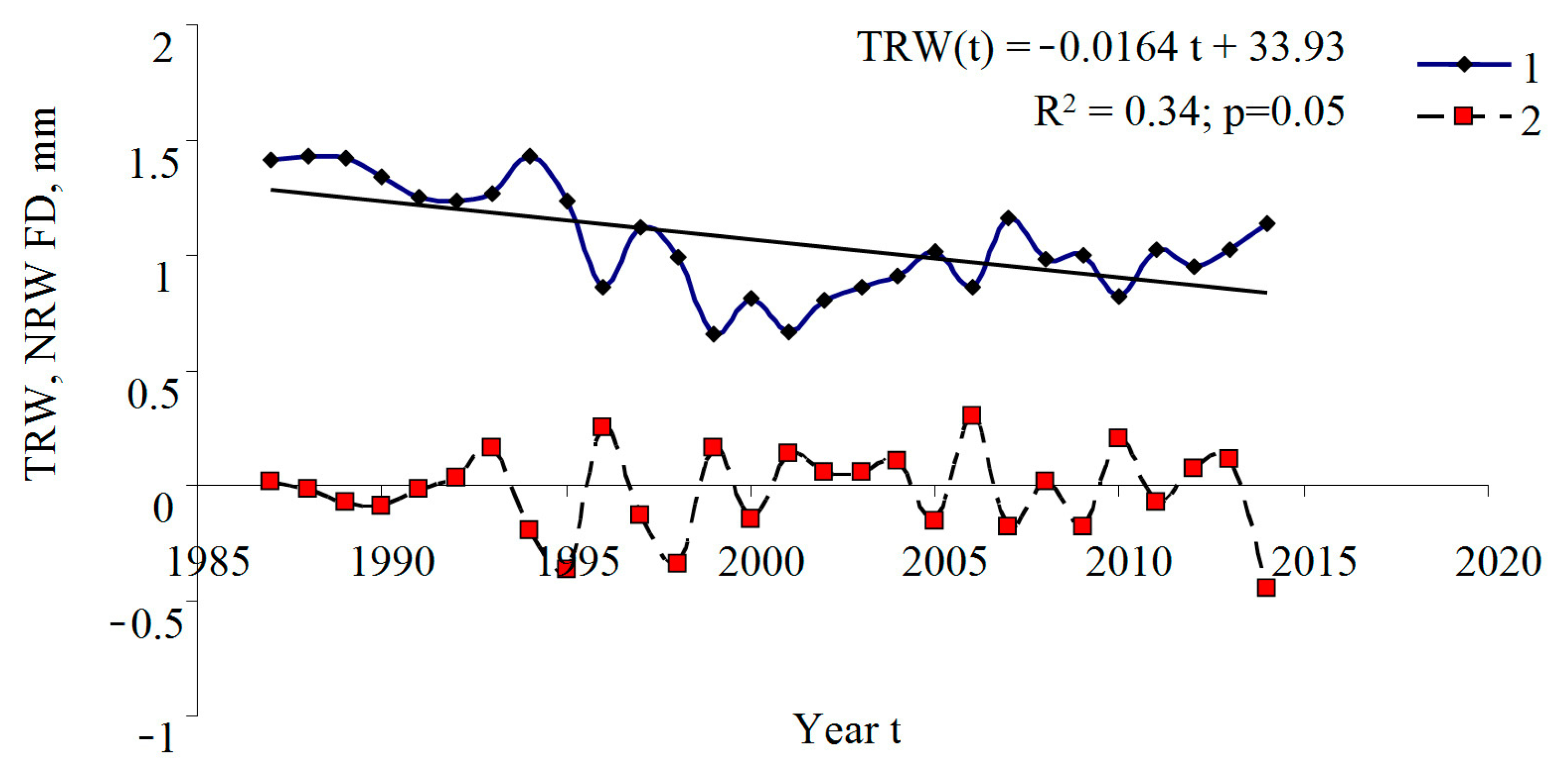
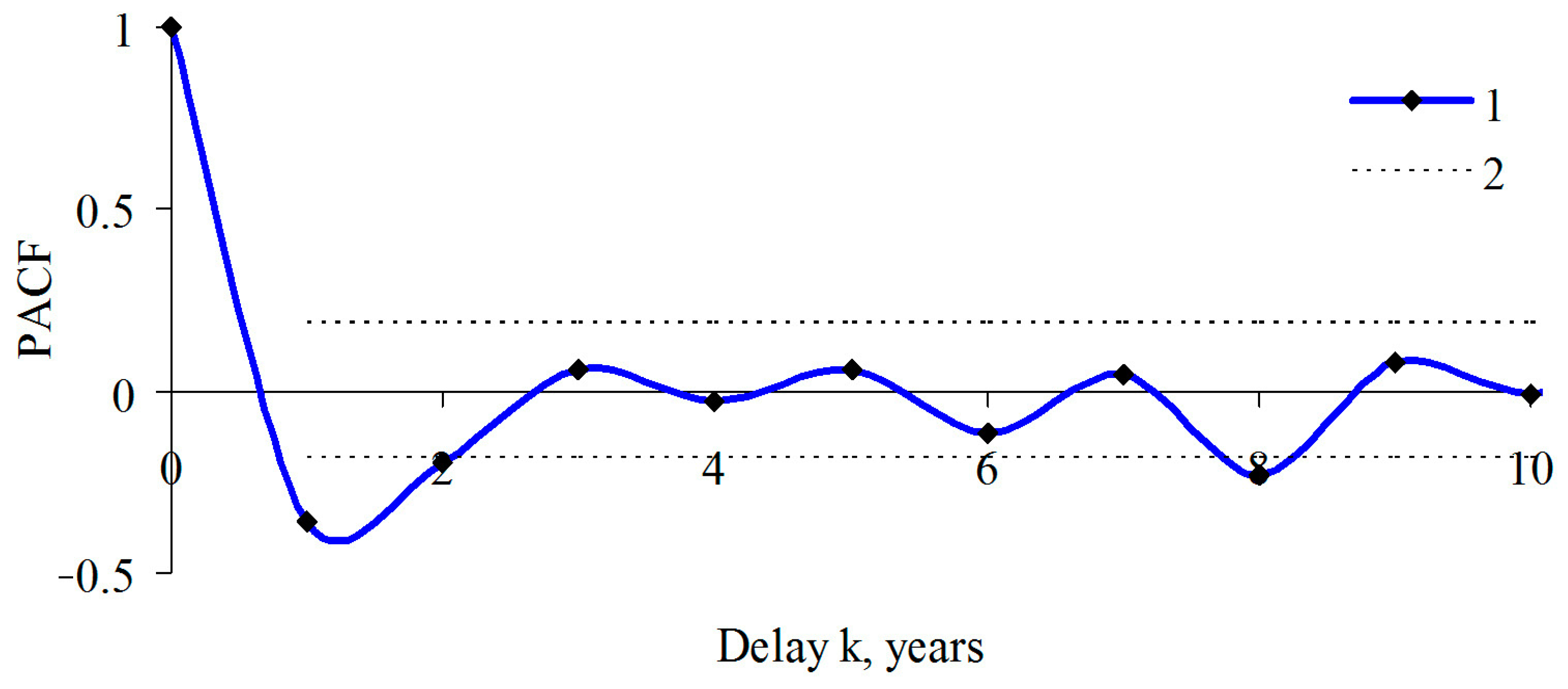
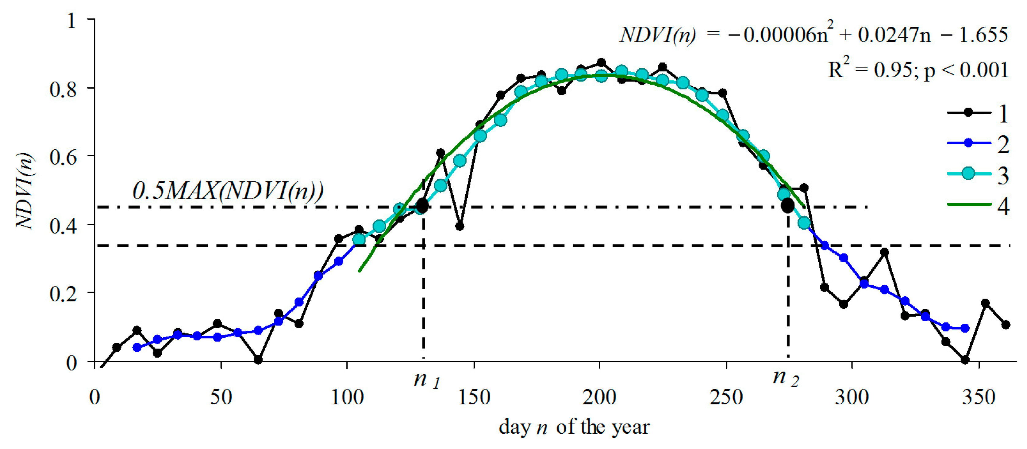
3. Results
4. Discussion
5. Conclusions
Supplementary Materials
Author Contributions
Funding
Acknowledgments
Conflicts of Interest
References
- Dobbertin, M. Tree growth as indicator of tree vitality and of tree reaction to environmental stress: A review. Eur. J. For. Res. 2005, 124, 319–333. [Google Scholar] [CrossRef]
- Barber, V.A.; Juday, G.P.; Finney, B.P. Reduced growth of Alaskan white spruce in the twentieth century from temperature-induced drought stress. Glob. Planet. Chang. 2008, 60, 289–305. [Google Scholar] [CrossRef]
- Lloyd, A.H.; Fastie, C.L. Spatial and temporal variability in the growth and climate response of treeline trees in Alaska. Clim. Chang. 2002, 52, 481–509. [Google Scholar] [CrossRef]
- Hirota, M.; Holmgren, M.; Van Nes, E.H.; Scheffer, M. Global resilience of tropical forest and savanna to critical transitions. Science 2011, 334, 232–235. [Google Scholar] [CrossRef] [PubMed] [Green Version]
- Sarris, D.; Christodoulakis, D.; Körner, C. Recent decline in precipitation and tree growth in the eastern Mediterranean. Glob. Chang. Biol. 2007, 13, 1187–1200. [Google Scholar] [CrossRef]
- Williams, A.P.; Allen, C.D.; Macalady, A.K.; Griffin, D.; Woodhouse, C.A.; Meko, D.M.; Swetnam, T.W.; Rauscher, S.A.; Seager, R.; Grissino-Mayer, H.D.; et al. Temperature as a potent driver of regional forest drought stress and tree mortality. Nat. Clim. Chang. 2013, 3, 292–297. [Google Scholar] [CrossRef]
- Shestakova, T.A.; Gutiérrez, E.; Kirdyanov, A.V.; Camarero, J.J.; Génova, M.; Knorre, A.A.; Linares, J.C.; de Dios, V.R.; Sánchez-Salguero, R.; Voltas, J. Forests synchronize their growth in contrasting Eurasian regions in response to climate warming. Proc. Natl. Acad. Sci. USA 2016, 113, 662–667. [Google Scholar] [CrossRef] [Green Version]
- Sass-Klaassen, U.G.W.; Fonti, P.; Cherubini, P.; Gričar, J.; Robert, E.M.R.; Steppe, K.; Bräuning, A. A tree-centered approach to assess impacts of extreme climatic events on forests. Front. Plant Sci. 2016, 7, 1069. [Google Scholar] [CrossRef] [Green Version]
- Fritts, H.C. Tree Rings and Climate; Academic Press: London, UK, 1976; p. 567. [Google Scholar]
- Zuidema, P.A.; Frank, D. Forests: Tree rings track climate trade-offs. Nature 2015, 523, 531. [Google Scholar] [CrossRef] [Green Version]
- Babst, F.; Poulter, B.; Bodesheim, P.; Mahecha, M.D.; Frank, D.C. Improved tree-ring archives will support earth-system science. Nat. Ecol. Evol. 2017, 1, 1–2. [Google Scholar] [CrossRef]
- Gewehr, S.; Drobyshev, I.; Berninger, F.; Bergeron, Y. Soil characteristics mediate the distribution and response of boreal trees to climatic variability. Can. J. For. Res. 2014, 498, 487–498. [Google Scholar] [CrossRef] [Green Version]
- Vaganov, E.A.; Hughes, M.K.; Shashkin, A.V. Growth Dynamics of Conifer Tree Rings: Images of Past and Future Environments; Springer: New York, NY, USA, 2006; Volume 183, p. 354. [Google Scholar]
- Ketterings, Q.M.; Coe, R.; Van Noordwijk, M.; Ambagau, Y.; Palm, C.A. Reducing uncertainty in the use of allometric biomass equations for predicting above-ground tree biomass in mixed secondary forests. For. Ecol. Manag. 2001, 146, 199–209. [Google Scholar] [CrossRef]
- Van Breugel, M.; Ransijn, J.; Craven, D.; Bongers, F.; Hall, J.S. Estimating carbon stock in secondary forests: Decisions and uncertainties associated with allometric biomass models. For. Ecol. Manag. 2011, 262, 1648–1657. [Google Scholar] [CrossRef]
- Babst, F.; Bouriaud, O.; Alexander, R.; Trouet, V.; Frank, D. Toward consistent measurements of carbon accumulation: A multi-site assessment of biomass and basal area increment across Europe. Dendrochronologia 2014, 32, 153–161. [Google Scholar] [CrossRef]
- St. George, S. The global network of tree-ring widths and its applications to paleoclimatology. Pages 2014, 22, 16–17. [Google Scholar] [CrossRef] [Green Version]
- Babst, F.; Poulter, B.; Trouet, V.; Tan, K.; Neuwirth, B.; Wilson, R.; Carrer, M.; Grabner, M.; Tegel, W.; Levanic, T.; et al. Site- and species-specific responses of forest growth to climate across the European continent. Glob. Ecol. Biogeogr. 2013, 22, 706–717. [Google Scholar] [CrossRef]
- Baral, S.; Gaire, N.P.; Aryal, S.; Pandey, M.; Rayamajhi, S.; Vacik, H. Growth Ring Measurements of Shorea robusta Reveal Responses to Climatic Variation. Forests 2019, 10, 466. [Google Scholar] [CrossRef] [Green Version]
- Drobyshev, I.; Gewehr, S.; Berninger, F.; Bergeron, Y. Species specific growth responses of black spruce and trembling aspen may enhance resilience of boreal forest to climate change. J. Ecol. 2013, 101, 231–242. [Google Scholar] [CrossRef] [Green Version]
- Mérian, P.; Pierrat, J.-C.; Lebourgeois, F. Effect of sampling effort on the regional chronology statistics and climate-growth relationships estimation. Dendrochronologia 2013, 31, 58–67. [Google Scholar] [CrossRef]
- Camarero, J.J.; Franquesa, M.; Sangüesa-Barreda, G. Timing of drought triggers distinct growth responses in holm oak: Implications to predict warming-induced forest defoliation and growth decline. Forests 2015, 6, 1576–1597. [Google Scholar] [CrossRef] [Green Version]
- Vicente-Serrano, S.M. Evaluating the impact of drought using remote sensing in a Mediterranean, semi-arid region. Nat. Hazards 2007, 40, 173–208. [Google Scholar] [CrossRef]
- Büntgen, U.; Trouet, V.; Frank, D.; Leuschner, H.H.; Friedrichs, D.; Luterbacher, J.; Esper, J. Tree-ring indicators of German summer drought over the last millennium. Quat. Sci. Rev. 2010, 29, 1005–1016. [Google Scholar] [CrossRef]
- Hall, F.G.; Botkin, D.B.; Strebel, D.E.; Woods, K.D.; Goetz, S.J. Large-scale patterns of forest succession as determined by remote sensing. Ecology 1991, 72, 628–640. [Google Scholar] [CrossRef]
- Song, C.; Woodcook, C.E. Monitoring forest succession with multitemporal landsat images: Factors of uncertainty. IEEE Trans. Geosci. Remote Sens. 2003, 41, 2557–2567. [Google Scholar] [CrossRef]
- Tucker, C.J.; Sellers, P.J. Satellite remote sensing of primary production. Int. J. Remote Sens. 1986, 7, 1395–1416. [Google Scholar] [CrossRef]
- Lu, D. The potential and challenge of remote sensing-based biomass estimation. Int. J. Remote Sens. 2006, 27, 1297–1328. [Google Scholar] [CrossRef]
- Timothy, D.; Onisimo, M.; Cletah, S.; Adelabu, S.; Tsitsi, B. Remote sensing of above ground forest biomass: A review. Trop. Ecol. 2016, 57, 125–132. [Google Scholar]
- Crowther, T.W.; Glick, H.B.; Covey, K.R.; Bettigole, C.; Maynard, D.S.; Thomas, S.M.; Smith, J.R.; Hintler, G.; Duguid, M.C.; Amatulli, G.; et al. Mapping tree density at a global scale. Nature 2015, 525, 201–205. [Google Scholar] [CrossRef] [PubMed]
- Myneni, R.B.; Hall, F.G.; Sellers, P.J.; Marshak, A.L. The meaning of spectral vegetation indices. IEEE Trans. Geosci. Remote Sens. 1995, 33, 481–486. [Google Scholar] [CrossRef]
- Babst, F.; Bodesheim, P.; Charney, N.; Friend, A.D.; Girardin, M.P.; Klesse, S.; Moore, D.J.P.; Seftigen, K.; Björklund, J.; Bouriaud, O.; et al. When tree rings go global: Challenges and opportunities for retro- and prospective insight. Quat. Sci. Rev. 2018, 197, 1–20. [Google Scholar] [CrossRef]
- Bunn, A.G.; Hughes, M.K.; Kirdyanov, A.V.; Losleben, M.; Shishov, V.V.; Berner, L.T.; Oltchev, A.; Vaganov, E.A. Comparing forest measurements from tree rings and a space-based index of vegetation activity in Siberia. Environ. Res. Lett. 2013, 8, 035034. [Google Scholar] [CrossRef]
- Vicente-Serrano, S.M.; Camarero, J.J.; Olano, J.M.; Martín-Hernández, N.; Peña-Gallardo, M.; Tomás-Burguera, M.; Gazol, A.; Azorin-Molina, C.; Bhuyan, U.; Kenawy, A. Diverse relationships between forest growth and the Normalized Difference Vegetation Index at a global scale. Remote Sens. Environ. 2016, 187, 14–29. [Google Scholar] [CrossRef] [Green Version]
- Beck, P.S.A.; Andreu-Hayles, L.; D’Arrigo, R.D.; Anchukaitis, K.J.; Tucker, C.J.; Pinzón, J.E.; Goetz, S.J. A large-scale coherent signal of canopy status in maximum latewood density of tree rings at arctic treeline in North America. Glob. Planet. Chang. 2013, 100, 109–118. [Google Scholar] [CrossRef]
- Berner, L.T.; Beck, P.S.A.; Bunn, A.G.; Goetz, S.J. Plant response to climate change along the forest-tundra ecotone in northeastern Siberia. Glob. Chang. Biol. 2013, 19, 3449–3462. [Google Scholar] [CrossRef] [PubMed]
- Lopatin, E.; Kolström, T.; Spiecker, H. Determination of forest growth trends in Komi Republic (northwestern Russia): Combination of tree-ring analysis and remote sensing data. Boreal Environ. Res. 2006, 11, 341–353. [Google Scholar]
- Decuyper, M.; Chávez, R.O.; Copini, P.; Sass-Klaassen, U. A multi-scale approach to assess the effect of groundwater extraction on Prosopis tamarugo in the Atacama Desert. J. Arid. Environ. 2016, 131, 25–34. [Google Scholar] [CrossRef]
- D’Arrigo, R.D.; Malmstrom, C.M.; Jacoby, G.C.; Los, S.O.; Bunker, D.E. Correlation between maximum latewood density of annual tree rings and NDVI based estimates of forest productivity. Int. J. Remote Sens. 2000, 21, 2329–2336. [Google Scholar] [CrossRef]
- Beck, P.S.A.; Goetz, S.J. Satellite observations of high northern latitude vegetation productivity changes between 1982 and 2008: Ecological variability and regional differences. Environ. Res. Lett. 2011, 6, 045501. [Google Scholar] [CrossRef]
- Pasho, E.; Alla, A.Q. Climate impacts on radial growth and vegetation activity of two co-existing Mediterranean pine species. Can. J. For. Res. 2015, 45, 1748–1756. [Google Scholar] [CrossRef] [Green Version]
- Kaufmann, R.K.; D’Arrigo, R.D.; Paletta, L.F.; Tian, H.Q.; Jolly, W.M.; Myneni, R.B. Identifying climatic controls on ring width: The timing of correlations between tree rings and NDVI. Earth Interact. 2008, 12, 1–14. [Google Scholar] [CrossRef] [Green Version]
- Huston, M.A.; Wolverton, S. The global distribution of net primary production: Resolving the paradox. Ecol. Monogr. 2009, 79, 343–377. [Google Scholar] [CrossRef]
- Soukhovolsky, V.; Ivanova, Y. Modeling production processes in forest stands: An adaptation of the Solow growth model. Forests 2018, 9, 391. [Google Scholar] [CrossRef] [Green Version]
- Suni, T.; Rinne, J.; Reissell, A.; Altimir, N.; Keronen, P.; Rannik, Ü.; Dal Maso, M.; Kulmala, M.; Vesala, T. Long-term measurements of surface fluxes above a Scots pine forest in Hyytiälä, southern Finland, 1996–2001. Boreal Environ. Res. 2003, 8, 287–301. [Google Scholar]
- Rossi, S.; Morin, H.; Deslauriers, A.; Plourde, P.Y. Predicting xylem phenology in black spruce under climate warming. Glob. Chang. Biol. 2011, 17, 614–625. [Google Scholar] [CrossRef]
- Kaufmann, R.K.; D’Arrigo, R.D.; Laskowski, C.; Myneni, R.B.; Zhou, L.; Davi, N.K. The effect of growing season and summer greenness on northern forests. Geophys. Res. Lett. 2004, 31, 3–6. [Google Scholar] [CrossRef]
- Avitabile, V.; Herold, M.; Heuvelink, G.B.M.; Lewis, S.L.; Phillips, O.L.; Asner, G.P.; Armston, J.; Ashton, P.S.; Banin, L.; Bayol, N.; et al. An integrated pan-tropical biomass map using multiple reference datasets. Glob. Chang. Biol. 2016, 22, 1406–1420. [Google Scholar] [CrossRef] [PubMed] [Green Version]
- Cuny, H.E.; Rathgeber, C.B.K.; Frank, D.; Fonti, P.; Makinen, H.; Prislan, P.; Rossi, S.; Martinez Del Castillo, E.; Campelo, F.; Vavrčik, H.; et al. Woody biomass production lags stem-girth increase by over one month in coniferous forests. Nat. Plants 2015, 1, 6. [Google Scholar] [CrossRef]
- Bhuyan, U.; Zang, C.; Vicente-Serrano, S.M.; Menzel, A. Exploring Relationships among Tree-Ring Growth, Climate Variability, and Seasonal Leaf Activity on Varying Timescales and Spatial Resolutions. Remote Sens. 2017, 9, 526. [Google Scholar] [CrossRef] [Green Version]
- Available online: http://web.utk.edu/~grissino/software.htm (accessed on 10 July 2020).
- Available online: https://earthdata.nasa.gov (accessed on 20 June 2020).
- Ivanova, Y.; Kovalev, A.; Yakubailik, O.; Soukhovolsky, V. The Use of Satellite Information (MODIS/Aqua) for Phenological and Classification Analysis of Plant Communities. Forests 2019, 10, 561. [Google Scholar] [CrossRef] [Green Version]
- Available online: https://aqua.nasa.gov/amsr-e (accessed on 10 July 2020).

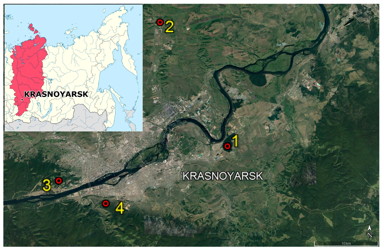
| Plot No. | Coordinates | Number of Trees | Mean Annual TRW, mm | Photograph |
|---|---|---|---|---|
| 1 | 56.043725° N 93.161901° E | 30 | 0.95 ± 0.076 |  |
| 2 | 56.222678° N 92.990675° E | 29 | 1.92 ± 0.13 |  |
| 3 | 55.994809° N 92.735070° E | 32 | 1.31 ± 0.07 |  |
| 4 | 55.963131° N 92.854473° E | 29 | 0.98 ± 0.08 |  |
| NDVI Matrix | G1 | G2 | G3 | G4 |
|---|---|---|---|---|
| a1 | 0.978 | −0.153 | 0.144 | 0.013 |
| a2 | −0.987 | 0.155 | 0.011 | 0.031 |
| a3 | 0.971 | −0.203 | −0.128 | 0.017 |
| 1−R2a | 0.710 | 0.704 | −0.008 | 0.001 |
| Eigenvalue | 3.377 | 0.585 | 0.037 | 0.001 |
| LST matrix | H1 | H2 | H3 | H4 |
| b1 | 0.985 | −0.009 | 0.173 | 0.012 |
| b2 | −0.995 | 0.097 | −0.017 | 0.022 |
| b3 | 0.957 | −0.226 | −0.181 | 0.010 |
| 1−R2b | 0.343 | 0.938 | −0.040 | 0.000 |
| Eigenvalue | 2.993 | 0.942 | 0.064 | 0.001 |
| NDVI | LST | |||
|---|---|---|---|---|
| Sample Plot | G1 | G1 + G2 | H1 | H1 + H2 |
| No. 1 | 84.42 | 99.04 | 74.83 | 98.37 |
| No. 2 | 72.07 | 96.02 | 74.52 | 99.07 |
| No. 3 | 81.37 | 99.06 | 77.22 | 99.83 |
| No. 4 | 88.46 | 98.99 | 80.78 | 99.72 |
| Coefficients | Sample Plot | |||
|---|---|---|---|---|
| No. 1 | No. 2 | No. 3 | No. 4 | |
| c0 | 0.050 | –0.030 | 0.013 | 0.015 |
| c1 | 0.049 * | –0.004 | 0.059 * | 0.052 * |
| c2 | –0.048 * | 0.052 * | –0.089 * | –0.069 * |
| c3 | –1.058 * | –0.535 * | –0.342 * | 0.445 * |
| R2 | 0.510 | 0.430 | 0.500 | 0.580 |
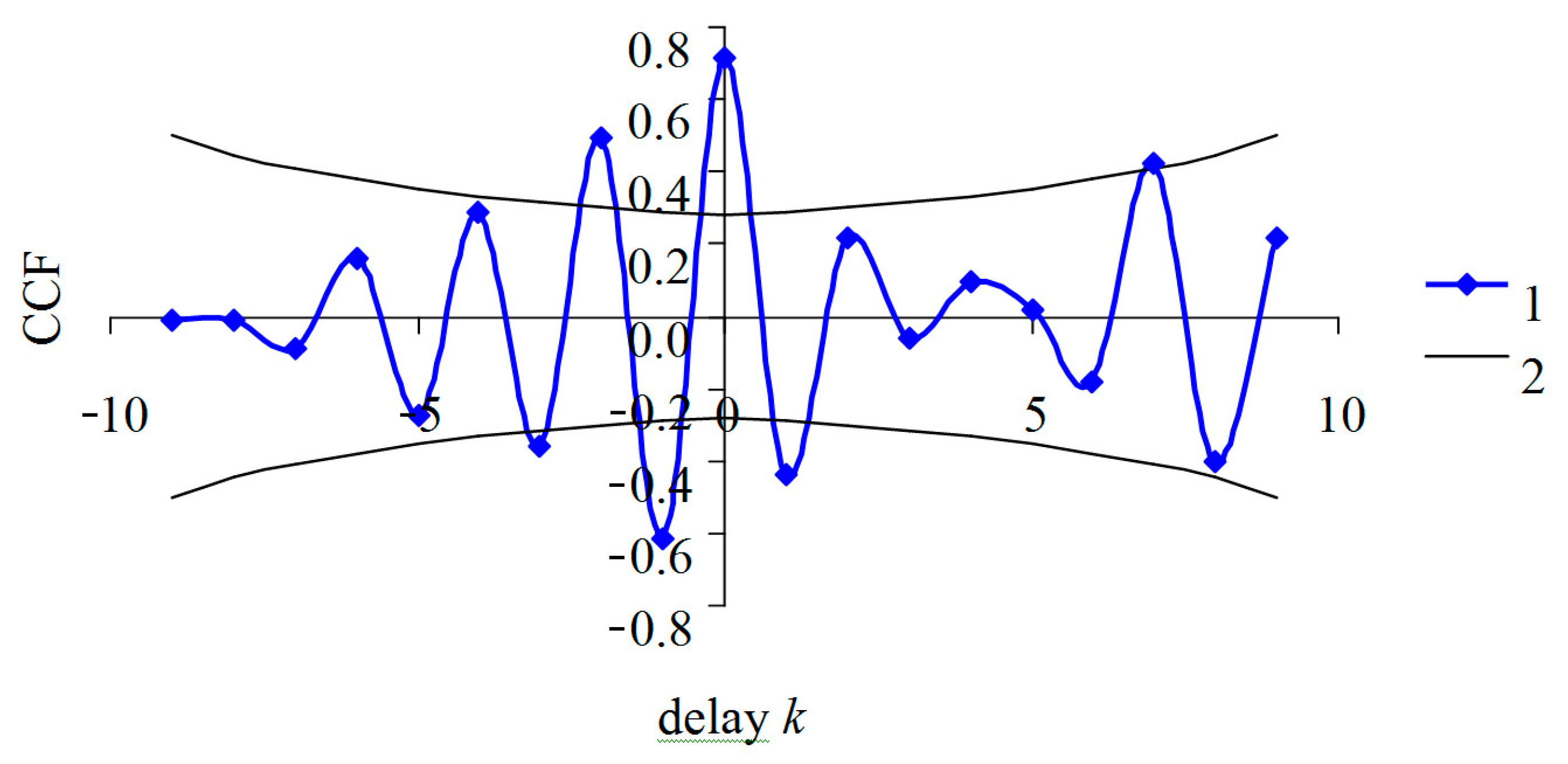
| CCF (k = 0) | 0.72 | 0.74 | 0.78 | 0.76 |
| Variable | Coefficient | Standard Error | t(9) | p-Level |
|---|---|---|---|---|
| c0 | 0.010 | 0.035 | 0.292 | 0.777 |
| G1 | 0.089 | 0.031 | 2.819 | 0.020 |
| H1 | –0.142 | 0.053 | –2.670 | 0.026 |
| TRW FD(t − 1) | –0.510 | 0.183 | –2.787 | 0.021 |
| R2 | 0.70 | |||
| p | 0.005 | |||
| CCF(k = 0) | 0.84 | |||
Publisher’s Note: MDPI stays neutral with regard to jurisdictional claims in published maps and institutional affiliations. |
© 2020 by the authors. Licensee MDPI, Basel, Switzerland. This article is an open access article distributed under the terms and conditions of the Creative Commons Attribution (CC BY) license (http://creativecommons.org/licenses/by/4.0/).
Share and Cite
Ivanova, Y.; Kovalev, A.; Soukhovolsky, V. Modeling the Radial Stem Growth of the Pine (Pinus sylvestris L.) Forests Using the Satellite-Derived NDVI and LST (MODIS/AQUA) Data. Atmosphere 2021, 12, 12. https://doi.org/10.3390/atmos12010012
Ivanova Y, Kovalev A, Soukhovolsky V. Modeling the Radial Stem Growth of the Pine (Pinus sylvestris L.) Forests Using the Satellite-Derived NDVI and LST (MODIS/AQUA) Data. Atmosphere. 2021; 12(1):12. https://doi.org/10.3390/atmos12010012
Chicago/Turabian StyleIvanova, Yulia, Anton Kovalev, and Vlad Soukhovolsky. 2021. "Modeling the Radial Stem Growth of the Pine (Pinus sylvestris L.) Forests Using the Satellite-Derived NDVI and LST (MODIS/AQUA) Data" Atmosphere 12, no. 1: 12. https://doi.org/10.3390/atmos12010012
APA StyleIvanova, Y., Kovalev, A., & Soukhovolsky, V. (2021). Modeling the Radial Stem Growth of the Pine (Pinus sylvestris L.) Forests Using the Satellite-Derived NDVI and LST (MODIS/AQUA) Data. Atmosphere, 12(1), 12. https://doi.org/10.3390/atmos12010012