Mobile Monitoring for the Spatial and Temporal Assessment of Local Air Quality (NO2) in the City of London


Abstract
1. Introduction
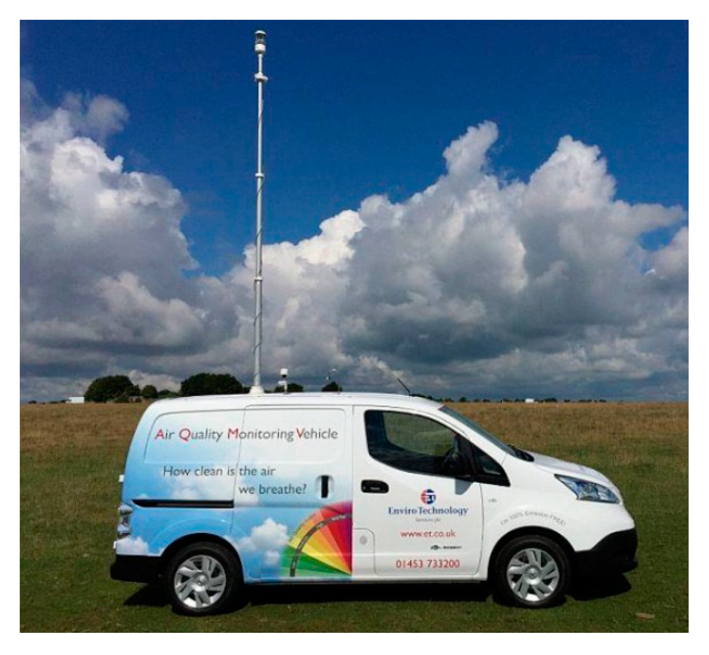
2. Experiments
- Data acquisition, cleaning and preparation; this included acquisition of both Smogmobile and Local Authority air quality data. Identification of gaps and errors and classification of the Smogmobile data in terms of static and dynamic (depending on whether the vehicle was stationary or moving).
- Spatial analysis of the Smogmobile data based on density plots (both at grid level and proximity distance from Local Authority monitoring systems (CMS and DT)).
- Statistical analysis of the result of the spatial outputs and assessment of the suitability of the dynamic monitoring system to provide useful insights for Local Authorities and to widely consider monitoring air quality in urban areas and to assess over time the impacts of strategies at a finer resolution.
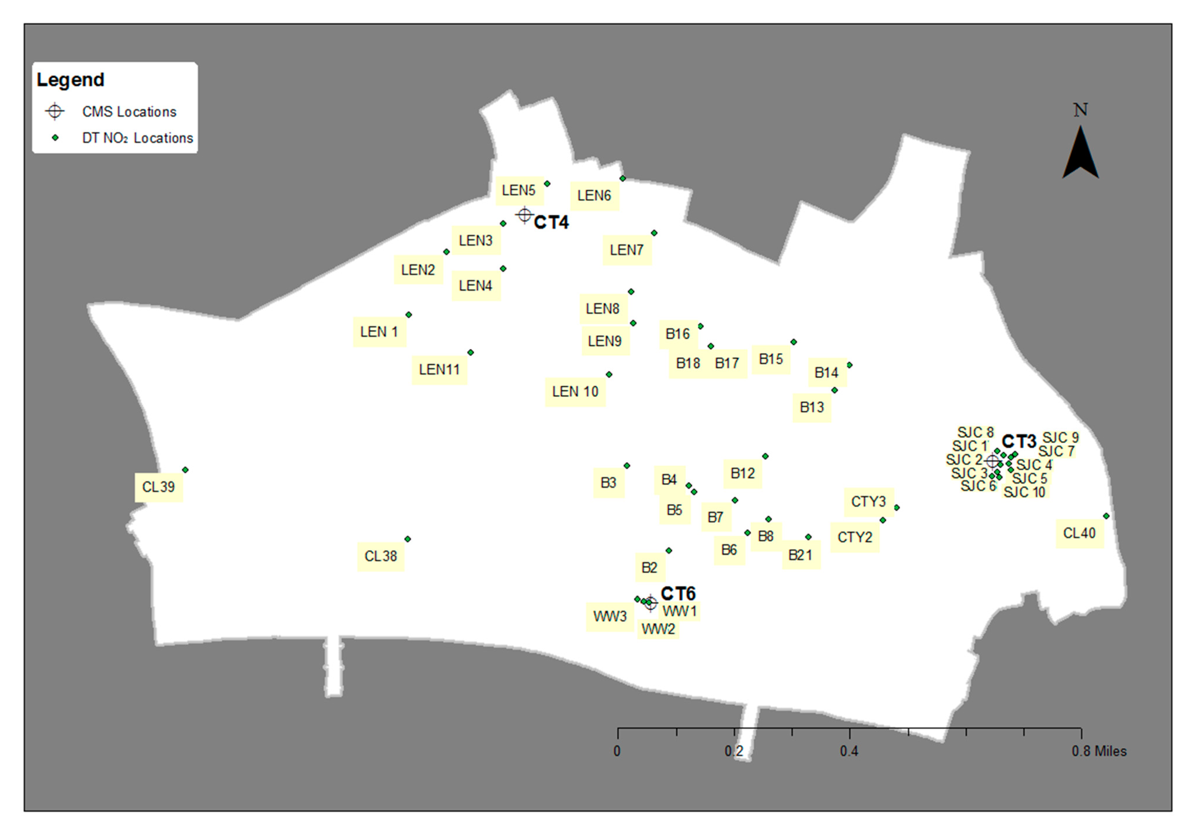
2.1. Case Study
2.2. Continous and Indicative Monitoring
- CT3: Sir John Cass School (east section of the City, near to Aldgate);
- CT4: Beech Street (north section of the City, within a road tunnel, near the Barbican estate); and,
- CT6: Walbrook Wharf (south section of City, near Cannon Street Station and the River Thames).
3. Results
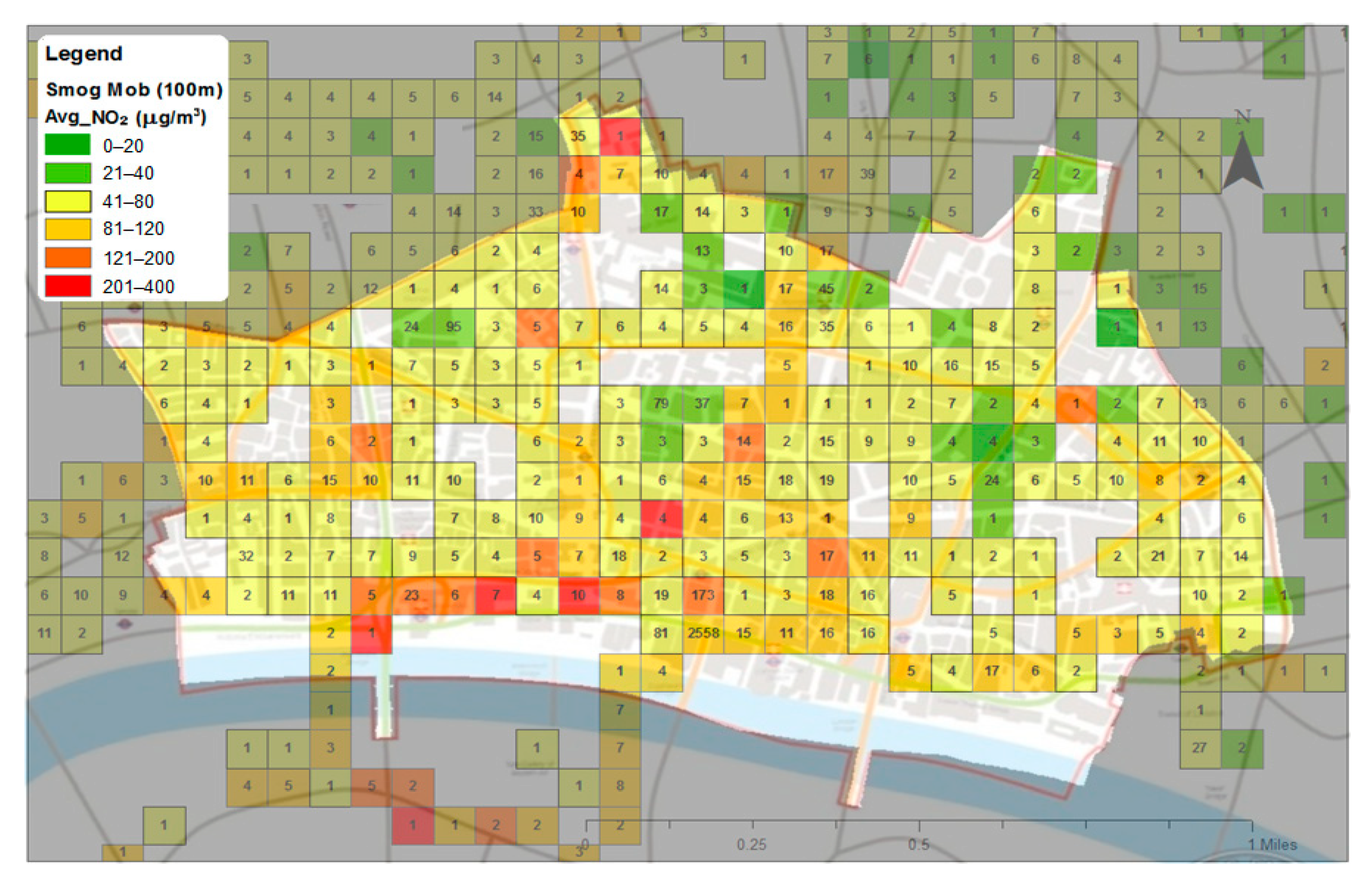
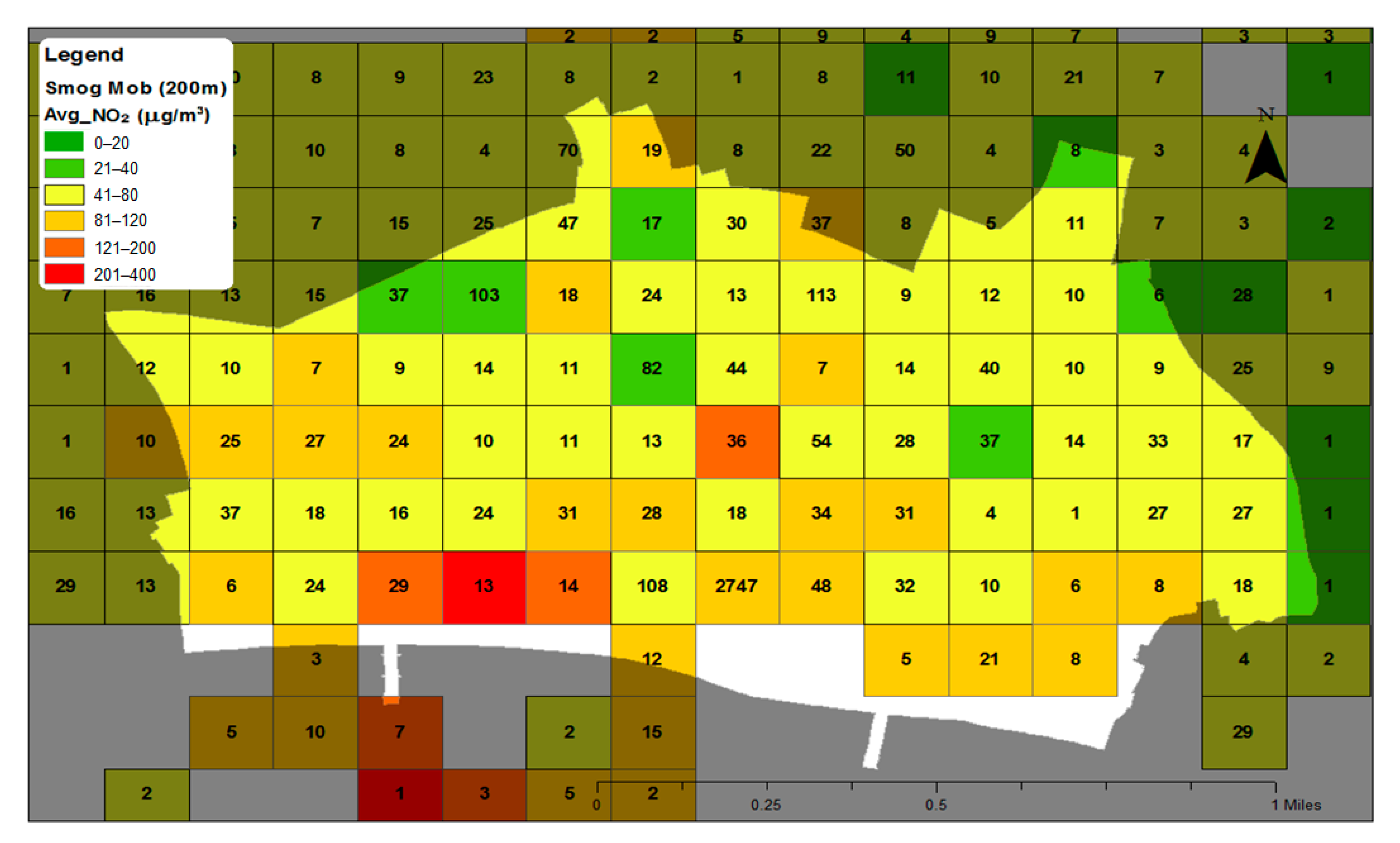
3.1. Spatial Density Analysis
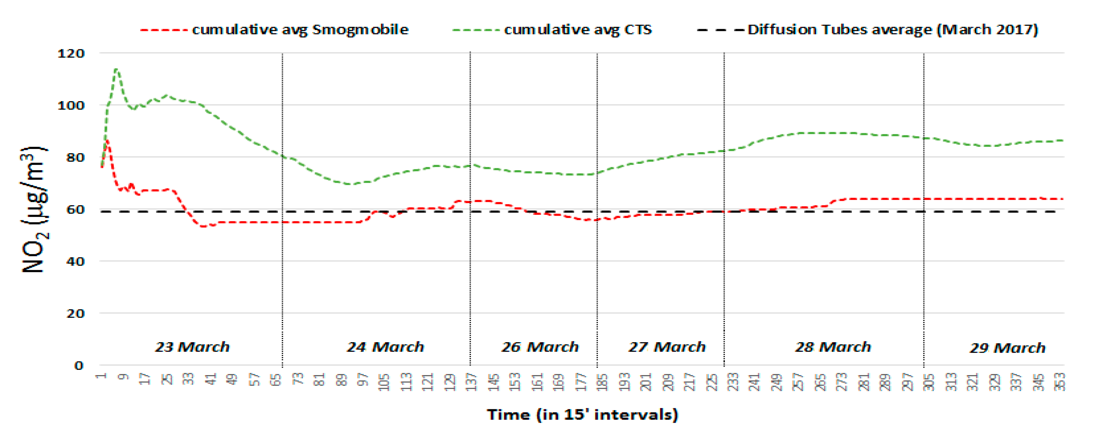
3.2. Time Series Analysis
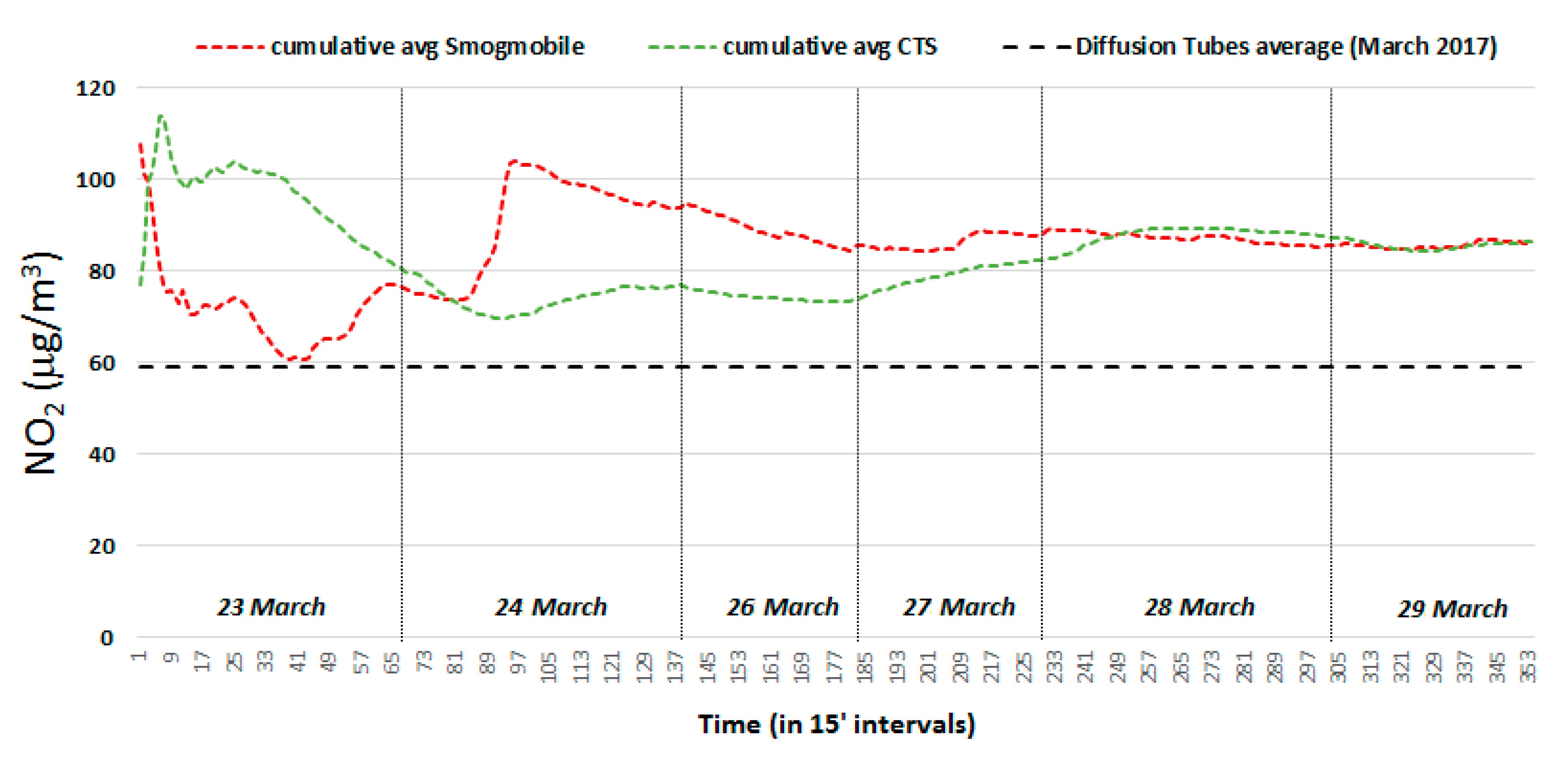
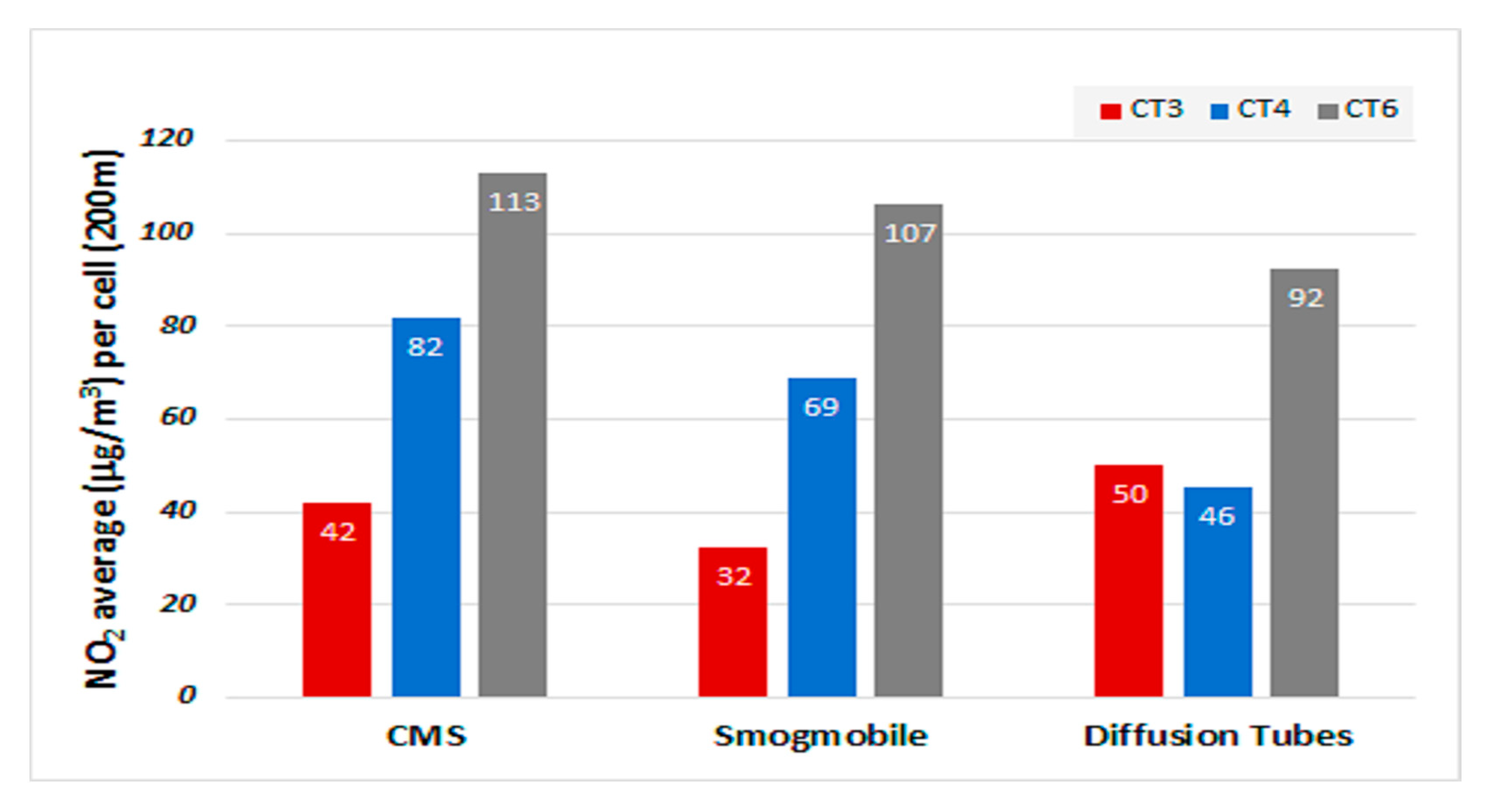
3.3. Comparative Analysis Smogmobile, CMS, and DTs
4. Discussion and Conclusions
- What is the most appropriate duration of a mobile campaign?
- What periods of the year should be targeted?
- Under which conditions and locations can the Smogmobile approach can be considered a potential alternative to, or simply complement, the traditional static monitoring methods?
- A predictive method for Local Authorities to anticipate, in the order of months, potential annual exceedances enabling timely interventions;
- Spatial and temporal representations of air quality across large areas or entire cities by using mobile monitoring techniques such as the Smogmobile.
5. Next Steps
Author Contributions
Funding
Data Availability Statement
Acknowledgments
Conflicts of Interest
Nomenclature
| CMS | Continuous Monitoring Stations (also named CT within the paper) |
| DT | Diffusion Tubes |
| CoL | City of London Corporation |
| NO2 | Nitrogen Dioxide |
References
- Meng, Q.Y.; Turpin, B.J.; Korn, L.; Weisel, C.P.; Morandi, M.; Colome, S.; Zhang, J.; Stock, T.; Spektor, D.; Winer, A.; et al. Influence of ambient (outdoor) sources on residential indoor and personal PM2.5 concentrations: Analyses of RIOPA data. J. Expo. Sci. Environ. Epidemiol. 2004, 15, 17–28. [Google Scholar] [CrossRef] [PubMed]
- Van Roosbroeck, S.; Li, R.; Hoek, G.; Lebret, E.; Brunekreef, B.; Spiegelman, D. Traffic-related outdoor air pollution and respiratory symptoms in children: The impact of adjustment for exposure measurement error. Epidemiology 2008, 19, 409–416. [Google Scholar] [CrossRef] [PubMed]
- Nagendra, S.S.; Yasa, P.R.; Mv, N.; Khadirnaikar, S.; Rani, P. Mobile monitoring of air pollution using low cost sensors to visualize spatio-temporal variation of pollutants at urban hotspots. Sustain. Cities Soc. 2019, 44, 520–535. [Google Scholar] [CrossRef]
- Minet, L.; Gehr, R.; Hatzopoulou, M. Capturing the sensitivity of land-use regression models to short-term mobile monitoring campaigns using air pollution micro-sensors. Environ. Pollut. 2017, 230, 280–290. [Google Scholar] [CrossRef] [PubMed]
- Suriano, D.; Prato, M.; Pfister, V.; Cassano, G.; Camporeale, G.; Dipinto, S.; Penza, M. Stationary and Mobile Low-Cost Gas Sensor-Systems for Air Quality Monitoring Applications. In Proceedings of the 4th Scientific Meeting EuNetAir 2015; Linkoping University: Linkoping, Sweden; Available online: https://www.ama-science.org/proceedings/details/2130 (accessed on 12 January 2021). [CrossRef]
- Zappi, P.; Bales, E.; Park, J.; Griswold, W.; Rosing, T. The citisense air quality monitoring mobile sensor node. In Proceedings of the 11th ACM/IEEE Conference on Information Processing in Sensor Networks, Beijing, China, 16–19 April 2012; Available online: https://www.researchgate.net/publication/267861564_The_CitiSense_Air_Quality_Monitoring_Mobile_Sensor_Node (accessed on 12 January 2021).
- Apte, J.S.; Messier, K.P.; Gani, S.; Brauer, M.; Kirchstetter, T.W.; Lunden, M.M.; Marshall, J.D.; Portier, C.J.; Vermeulen, R.C.; Hamburg, S.P. High-Resolution Air Pollution Mapping with Google Street View Cars: Exploiting Big Data. Environ. Sci. Technol. 2017, 51, 6999–7008. [Google Scholar] [CrossRef] [PubMed]
- Lim, C.C.; Kim, H.; Vilcassim, M.J.R.; Thurston, G.D.; Gordon, T.; Chen, L.-C.; Lee, K.; Heimbinder, M.; Kim, S.-Y. Mapping urban air quality using mobile sampling with low-cost sensors and machine learning in Seoul, South Korea. Environ. Int. 2019, 131, 105022. [Google Scholar] [CrossRef] [PubMed]
- Gelb, J.; Apparicio, P. Modelling Cyclists’ Multi-Exposure to Air and Noise Pollution with Low-Cost Sensors—The Case of Paris. Atmosphere 2020, 11, 422. [Google Scholar] [CrossRef]
- Mead, M.I.; Popoola, O.; Stewart, G.; Landshoff, P.V.; Calleja, M.; Hayes, M.J.; Baldovi, J.; McLeod, M.; Hodgson, T.; Dicks, J.; et al. The use of electrochemical sensors for monitoring urban air quality in low-cost, high-density networks. Atmos. Environ. 2013, 70, 186–203. [Google Scholar] [CrossRef]
- Snyder, E.G.; Watkins, T.H.; Solomon, P.A.; Thoma, E.D.; Williams, R.W.; Hagler, G.S.W.; Shelow, D.; Hindin, D.A.; Kilaru, V.J.; Preuss, P.W. The Changing Paradigm of Air Pollution Monitoring. Environ. Sci. Technol. 2013, 47, 11369–11377. [Google Scholar] [CrossRef] [PubMed]
- Department for Environment, Food and Rural Affairs (DEFRA). Clean Air Strategy. Available online: https://assets.publishing.service.gov.uk/government/uploads/system/uploads/attachment_data/file/770715/clean-air-strategy-2019.pdf (accessed on 12 January 2021).
- John, L.A. Air Pollution around Gloucestershire (20 June 2017); Enviro Technology Services Ltd.: London, UK, 2017. Available online: https://glostext.gloucestershire.gov.uk/documents/s39657/Air%20Quality%20Around%20Gloucestershire%20Schools%20Report%20FINAL%20200617%20ANNEX%20A.pdf (accessed on 12 January 2021).


| Date | Day | Location | Start Time | End Time | Duration | Sampling Mode |
|---|---|---|---|---|---|---|
| 23/March/2017 | Thursday | Walbrook Wharf Carpark | 07:07 | - | N.A. | N.A. |
| Fann Street | 08:23 | 08:57 | 00:34 | Outside, Roof | ||
| Appold Street | 09:47 | 09:50 | 00:03 | |||
| Guildhall Library | 10:16 | 10:49 | 00:33 | |||
| Walbrook Wharf Carpark | 11:20 | 13:14 | 01:54 | Outside, Roof | ||
| St Bartholomew’s Hospital | 14:04 | 16:10 | 02:06 | Outside, Roof | ||
| Fann Street | 16:17 | 16:25 | 00:08 | Outside, Roof & Kerb | ||
| Milton Street | 16:28 | 16:39 | 00:11 | |||
| St Katharine’s Way | 17:17 | 17:43 | 00:26 | |||
| Walbrook Wharf Carpark | - | 18:16 | N.A. | N.A. |
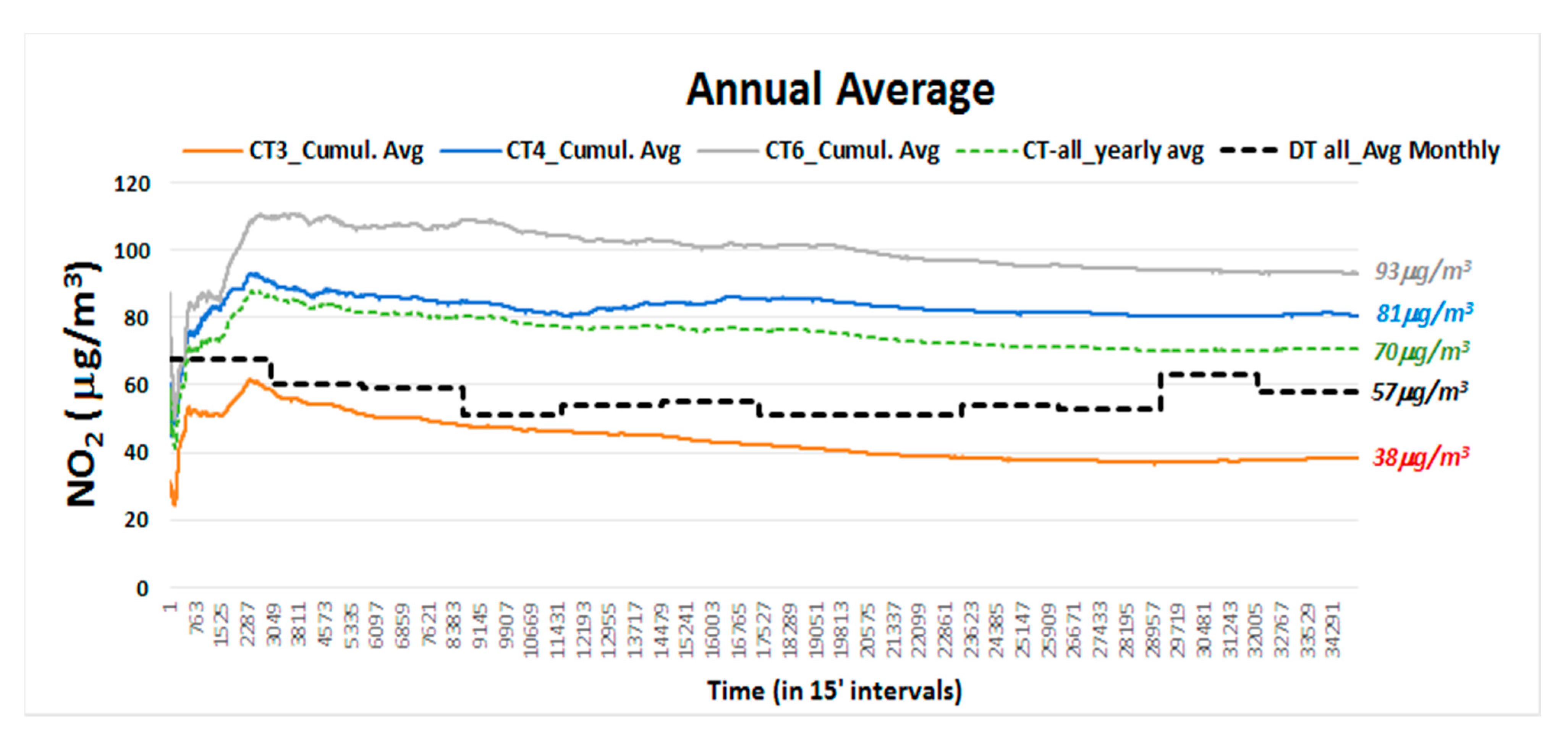
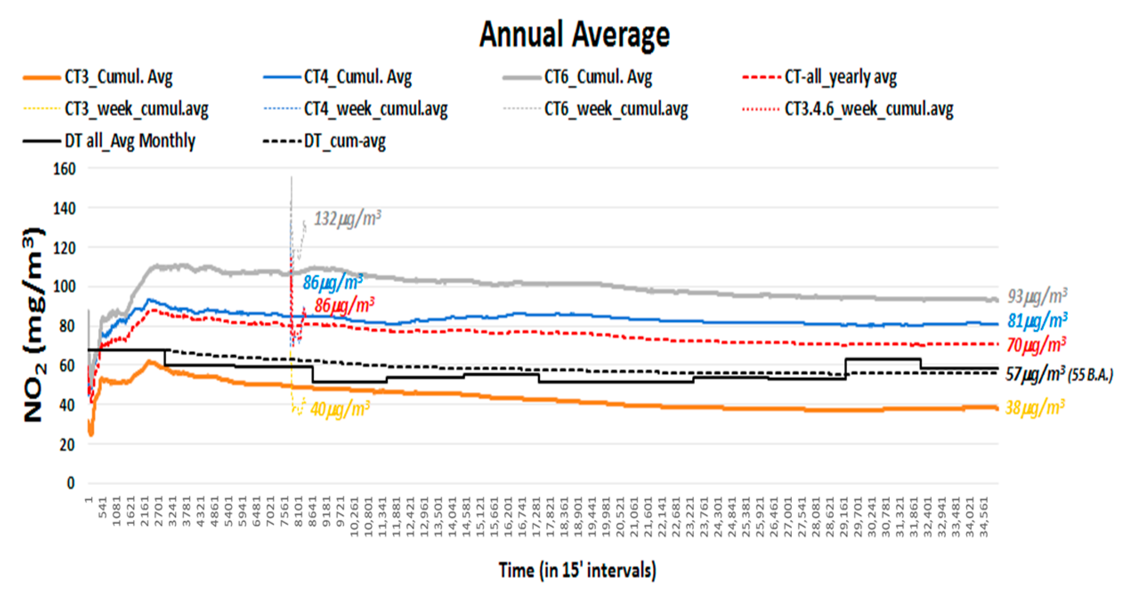
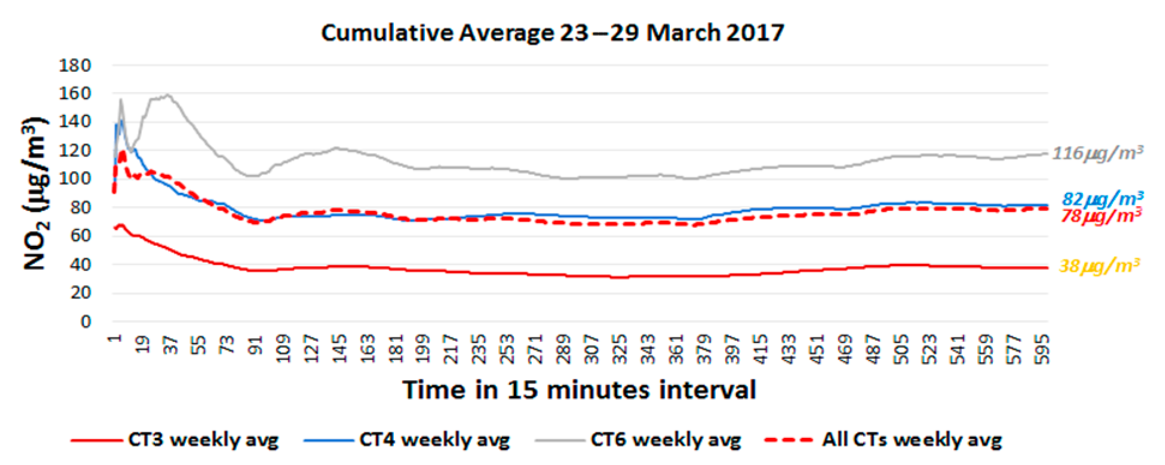
| Site ID * | Site Type * | Easting (X) * | Northing (Y) * | 2017 Annual Mean (µg/m3) * | (March 2017 Mean) ** | Data Capture (%) ** |
|---|---|---|---|---|---|---|
| CT3 (Sir John Cass School) | Urban Background | 533,475 | 181,187 | 38 | 42 | 98, (98) |
| CT4 (Beech Street) | Roadside | 532,176 | 181,862 | 81 | 82 | 99, (98) |
| CT6 (Walbrook Wharf) | Roadside | 532,528 | 180,784 | 93 | 113 | 97, (98) |
Publisher’s Note: MDPI stays neutral with regard to jurisdictional claims in published maps and institutional affiliations. |
© 2021 by the authors. Licensee MDPI, Basel, Switzerland. This article is an open access article distributed under the terms and conditions of the Creative Commons Attribution (CC BY) license (http://creativecommons.org/licenses/by/4.0/).
Share and Cite
Galatioto, F.; Ferguson-Moore, J.; Calderwood, R. Mobile Monitoring for the Spatial and Temporal Assessment of Local Air Quality (NO2) in the City of London. Atmosphere 2021, 12, 106. https://doi.org/10.3390/atmos12010106
Galatioto F, Ferguson-Moore J, Calderwood R. Mobile Monitoring for the Spatial and Temporal Assessment of Local Air Quality (NO2) in the City of London. Atmosphere. 2021; 12(1):106. https://doi.org/10.3390/atmos12010106
Chicago/Turabian StyleGalatioto, Fabio, James Ferguson-Moore, and Ruth Calderwood. 2021. "Mobile Monitoring for the Spatial and Temporal Assessment of Local Air Quality (NO2) in the City of London" Atmosphere 12, no. 1: 106. https://doi.org/10.3390/atmos12010106
APA StyleGalatioto, F., Ferguson-Moore, J., & Calderwood, R. (2021). Mobile Monitoring for the Spatial and Temporal Assessment of Local Air Quality (NO2) in the City of London. Atmosphere, 12(1), 106. https://doi.org/10.3390/atmos12010106