Vortex Initialization in the NCEP Operational Hurricane Models

Abstract

This paper describes the vortex initialization (VI) currently used in NCEP operational hurricane models (HWRF and HMON, and possibly HAFS in the future). The VI corrects the background fields for hurricane models: it consists of vortex relocation, and size and intensity corrections. The VI creates an improved background field for the data assimilation and thereby produces an improved analysis for the operational hurricane forecast. The background field after VI can be used as an initial field (as in the HMON model, without data assimilation) or a background field for data assimilation (as in HWRF model).

1. Introduction

Although dynamic prediction models have significantly advanced tropical cyclone (TC) track forecast guidance in past decades, the intensity guidance still relies heavily on statistical models or a combination of dynamic/statistical models. The primary challenges in initializing TCs in numerical models are the scarcity of in-situ observational data, the difficulties of using satellite data in the rain-intensive hurricane environment and the large differences between the observed and background storm structures in the data assimilation process, to which inaccuracies in model physics also contribute.

Generally speaking, there are three approaches of initializing TCs in dynamic prediction models. One approach is to apply a “bogus vortex” to the TC initial condition by prescribing the vortex structure and intensity based on the available real-time TC position and maximum surface wind [1,2,3,4]. The second approach is to create empirical synthetic data for the data analysis system to complement the sparse in-situ observations in the vicinity of the TC [5,6,7,8,9]. The third approach is the dynamic initialization, where TC vortex is initialized using Newtonian relaxation to some prescribed state [10,11,12,13]. The last two approaches have been explored to initialize TCs in operational dynamic models at the National Centers for Environmental Prediction (NCEP) [5,10]. More recently, in the research community, initializing the TC vortex based on advanced data assimilation techniques has begun. However, this approach is still in the research stage under the Hurricane Forecast Improvement Project (HFIP) [14] because: (1) the demonstrated improvements in forecast skill are very limited; and (2) critical operational forecast requirements of data availability in the operational framework and feasibility within the currently available computational resources have not been met.

In recent years, a Vortex Initialization (VI) scheme was successfully developed and implemented in the Hurricane Weather Research and Forecasting model (HWRF) at NCEP, and later adapted for the Hurricanes in a Multi-scale Ocean-coupled Non-hydrostatic model (HMON). The VI scheme is based on the vortex separation method developed by Kurihara et al. 1995 [15] for the Geophysical Fluid Dynamics Laboratory (GFDL) hurricane model. Instead of implanting a spun-up vortex from a simplified dynamic model, the VI scheme modifies the intensity and storm structure of the separated vortex and then relocates it to the in situ position in the background fields. The modification and relocation of the vortex is based on the NHC-estimated real-time TC position and intensity at the surface from the Tropical Cyclone Vitals Database (TCVitals). TCVitals is an archive of Cyclone Message Files, which contain information such as cyclone location, intensity, horizontal wind, and pressure structure, and depth of convection, and is created in real time by forecasting centers. The VI scheme greatly reduces the false spin-up/spin-down problem caused by inconsistencies between the initial conditions and the model dynamics and physics. The background field modified by VI can be used as an initial field without data assimilation (as in HMON), or as a first guess field for the data assimilation (as in HWRF).

In 2007, the NCEP HWRF team implemented a full vortex initialization (FVI) scheme in the HWRF system. The FVI scheme consists of two major steps: (1) reconstructing the background fields as in the VI scheme above; and (2) applying a data assimilation technique such as Grid-point Statistical Interpolation (GSI) [16] to assimilate available new observations, especially flight observations, to further improve the storm structure and environment flow. If there are no data, or very few data, near the hurricane, the FVI scheme can still generate the full initial conditions for TC track and intensity forecasts. When observational data from aircraft reconnaissance or other platforms are available, the vortex structure and its environment flow can be further improved through data assimilation.

The HWRF cycling system is described in the next section. The three steps in the VI scheme (vortex separation, storm size correction and storm intensity correction) are presented in Section 3. The bogus vortex used to correct weak storms is described briefly in Section 4. Application of the VI in the HWRF system is given in Section 5. The results are presented in Section 6, followed by discussion and conclusions in Section 7.

2. The HWRF Cycling System

The HRWF is cycled four times daily at 00, 06, 12 and 18 UTC and uses GFS boundary conditions. The GFS analysis is used to initialize the HWRF environmental fields (outermost domain) at every forecast cycle. The original HWRF initialization [17] also cycled the environmental fields and applied the vortex relocation technique [18,19,20] at each cycle. However, results showed that the HWRF environmental flow drifted away from that in the GFS and that this error increased as the number of cycles increased.

The HWRF Data Assimilation System (HDAS) [21] is used for the inner nest data assimilation. HDAS is basically the same as the Global Data Assimilation System (GDAS). Both systems follow similar procedures but are run on different model grids (global for GDAS and regional for HDAS). Both GDAS and HDAS employ the community GSI, which is supported by the Developmental Testbed Center (DTC). The background fields for HDAS are derived from the 6-h forecast of the HWRF (or GFS if no HWRF forecast exists).

The HWRF is a triple nested forecast system with the centers of the two nested domains moving along with predicated path of the storm. The initial outer and inner domain locations are based on the observed hurricane current and projected center positions and are, therefore, typically not the same from one cycle to the next. Once the domains have been defined, the VI and the HDAS are used to create the initial fields. If a previous 6-h HWRF forecast is available and the observed maximum wind speed of the storm is greater than or equal to 14 ms⁻¹, then the tropical cyclone vortex is extracted from that forecast and corrected to be included in the current initialization. If the previous HWRF forecast is not available or the observed maximum wind speed is less than 14 ms⁻¹, the same procedure is used except that the GFS vortex is corrected and added back into the initial fields. The detailed steps performed in each HWRF cycle are described in Appendix A.

3. Vortex Initialization

The vortex initialization procedure described in this paper is based on vortex cycling in a continuous assimilation mode (warm start). If a 6-h forecast from the previous cycle is available, then the vortex component is extracted from that forecast and the vortex initialization is performed. The corrected vortex is inserted back into the background field at the observed location. In the absence of the previous forecast cycle, a GFS vortex (or HDAS vortex if HDAS is applied to the parent domain) is used as a guess vortex and is subjected to the same vortex initialization as in the warm start mode. In the following subsections, we will discuss the details of the vortex cycling and initialization technique. Section 3.1 describes the vortex separation from its environmental field. Section 3.2 gives the details of storm size correction and its effect on the surface pressure, temperature and water vapor adjustments. Section 3.3 discusses the details of the storm intensity correction.

3.1. Separation of the Vortex from Its Environmental Fields

Before describing the vortex separation technique, we define some frequently used terms in this paper. The composite vortex refers to an axisymmetric storm which is created from a collection of model forecasts for various tropical storms. The bogus storm is created from the composite vortex by smoothing and performing size (and/or intensity) corrections. The background field, or guess field, is the 6-h model forecast from previous cycle or the output of the vortex initialization procedure, to which we can add observational data through data assimilation. The environmental field is defined as the background field after removing the vortex component.

Following [10,15], the original wind field at model sigma level = 0.85 (approximately 850 hPa) is used to define the filter domain. The wind field at sigma = 0.85 is first split into the basic field and the disturbance field. The disturbance field is used to define the filter domain which confines the hurricane component (vortex). The filter domain is estimated by examining the profile of the tangential wind component along each of the 24 radial directions (every 15 degrees) with respect to the storm center. The filter domain need not be circular (or symmetric); it may take a polygon shape. After the filter domain is defined, the optimum interpolation (see Appendix B of [15]) is used to estimate the non-hurricane component based on the non-hurricane values along the lateral boundary of the filter domain, and the environmental field is defined by (environmental field) = (basic field) + (non-hurricane component).

The environmental field is identical to the original field outside the filter domain. Next, we subtract the environmental field from the original field to obtain the vortex on high-resolution model grids. Using the same filter domain and assuming the filter domain is independent of height, the same procedure is applied for other variables such as MSLP (mean sea-level pressure), zonal and meridional wind components, temperature, and mixing ratio of water vapor to obtain the 3D vortex (a separation of the vortex for all 3D variables is carried out at each pressure level).

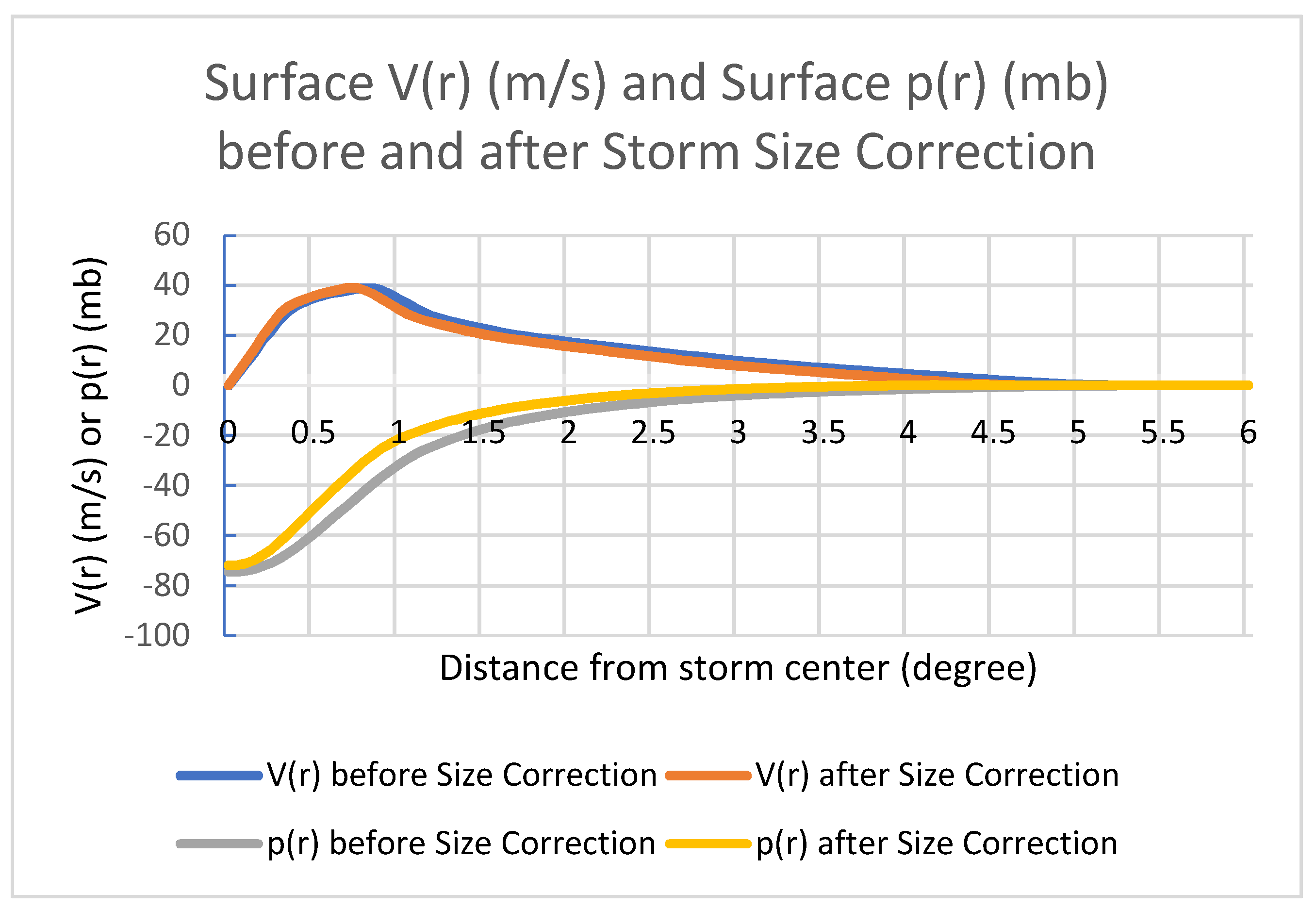
3.2. Storm Size Correction

For hurricane data assimilation we need a good background field. Storms in the background field can be too large or too small compared to the observed sizes. Storm size corrections were first introduced in the 2007 operational HWRF model (27 km for the parent, 9 km for the nest). Since then, overpredicted eyewall sizes often produced bad track and intensity forecasts as the eyewalls were continuing to expand during the model forecasts. This problem was largely solved by the introduction of the third nest (3 km) and the change of the boundary layer physics [22].

For storm size corrections, we use radial grid transformation. There are some early works in this area and the radial grid transformation has been used for different purposes (for example, [23]). The radial grid transformation approach used in this study is simple and straightforward. It uses two observation parameters, namely, the radius of maximum wind (RMW), denoted by $r_o$, and the radius of the outermost closed isobar (ROCI) (or R34, radius of the 34 knot wind speed, if available), denoted by $R_o$. The storm size correction can be achieved by stretching/compressing the model grid along the radial direction, and the stretching/compressing rate can be a linear function of the radial distance from the storm vortex center as defined by:

$${\alpha }_i=\frac{\Delta r_i^{*}}{\Delta r_i}=a+b{r}_i,$$

(1)

where a and b are constants, r and $r^{*}$ are the distances from the storm vortex center before and after the model grid is stretched. Index i represents the ith grid point, $\Delta r_i^{*}$ and $\Delta r_i$ are the small increments at the ith grid point. The two constants a and b can be determined from the two observation parameters $r_o$ and $R_o$ as follows.

Integrating Equation (1), we have:

$$r^{*}=f\left(r\right)={\int }_0^r\alpha \left(r\right)dr={\int }_0^r\left(a+br\right)dr=ar+\frac{1}{2}b{r}^2,$$

(2)

We compress/stretch the model grids such that:

$$r^{*}=f\left(r_m\right)=r_o \mathrm{at} r=r_m,$$

(3)

$$r^{*}=f\left(R_m\right)=R_o \mathrm{at} r=R_m,$$

(4)

where $r_m$ and $R_m$ denote the radius of the maximum wind and radius of the outermost closed isobar (or R34, the radius of the 34 knot wind speed) for the storm in the background field (or 6 h HWRF forecast field), respectively. Substituting Equations (3) and (4) into Equation (2), and solving for a and b, we have:

$$a=\frac{r_o{R}_m^2-r_m^2{R}_o}{R_m{r}_m\left(R_m-r_m\right)}, b=2\frac{R_o{r}_m-R_m{r}_o}{R_m{r}_m\left(R_m-r_m\right)},$$

(5)

and:

$$r^{*}=f\left(r\right)=\frac{r_o{R}_m^2-r_m^2{R}_o}{R_m{r}_m\left(R_m-r_m\right)}r+\frac{R_o{r}_m-R_m{r}_o}{R_m{r}_m\left(R_m-r_m\right)}{r}^2,$$

(6)

We set the storm size correction limit to be 15%, i.e., $0.85\le r_o/r_m\le 1.15$, and $0.85\le R_o/R_m\le 1.15$. If the storm size is significantly different from the observations, the 15% limit means that we do not match the observed storm size. The reason we set the limit is to make the vortex initialization as model-consistent as possible. Generally speaking, a large correction will cause a large adjustment in the model forecasts and should be avoided if possible.

In the special case of α = constant with b = 0, we have:

$$\alpha ={\alpha }_m=\frac{r_o}{r_m}=\frac{R_o}{R_m},$$

(7)

In this case, the storm size correction is based on one parameter only (this procedure was used in the initial implementation of the operational HWRF model in 2007).

To calculate the radius of the outermost closed isobar in the background fields, it is necessary to first adjust the minimum surface pressure to the observed value. Similarly, to calculate the radius of 34 knot winds, we also need to adjust the maximum wind speed for the background vortex (and composite vortex if bogus storm is used) to the observation value before searching for the R34 for both vortices (for a detailed calculation of R34 and ROCI, please refer to the DTC document).

Storm size corrections can often become problematic. The reason is that the eyewall size produced in the model can be much larger than the observed size, and the model does not support the observed small-size eyewall mainly due to a coarse horizontal resolution (and model physics). For example, the observed radius of maximum wind for 2005 Wilma remained about 9 km at 140 knots for many cycles. The model-produced radius of maximum wind was about 19 km. If we compress the radius of maximum winds to 9 km, the eyewall will collapse and significant spin-down will occur. Hence, the minimum value for a storm eyewall is currently set to 19 km and the correction of the storm size is limited to 15%.

The storm size correction affects the divergence and vorticity fields. Since the size correction is generally very small, no significant changes are expected for these fields. In the case where α = constant (b = 0), the divergence and vorticity will be the original values divided by the constant α = a.

3.2.1. Surface Pressure Adjustment after the Storm Size Correction

In our approximation of surface pressure, we only correct the axisymmetric part of the storm (generally speaking, the correction is small). The governing equation for the axisymmetric components along the radial direction is:

$$\frac{\partial u}{\partial t}+u\frac{\partial u}{\partial r}+w\frac{\partial u}{\partial z}-v\left(\frac{v}{r}+f_0\right)+\frac{1}{\rho } \frac{\partial p}{\partial r}=F_r,$$

(8)

where u, v, and w are the radial, tangential and vertical velocity components, respectively, $F_r\approx -C_d\frac{u}{H_B}v$ is the friction and $H_B$ is the height of the boundary layer, C_d is the momentum drag coefficient. $F_r$ can be estimated as $F_r\approx -{10}^{-6}v$ away from the storm center, and as $F_r\approx -{10}^{-5}v$ near the storm center. Dropping the friction and Lagrangian time derivative terms, Equation (8) gives the gradient wind balance.

Since we separate the hurricane component from its environment, the contribution from the environment flow to the average tangential wind speed can be neglected. From now on, the tangential velocity we discussed is referred to as the vortex component. We define the gradient wind stream function Ψ by:

$$\frac{\partial \Psi }{\partial r}=\frac{v^2}{r{f}_0}+v,$$

(9)

so:

$$\Psi ={\int }_{\infty }^r\left(\frac{v^2}{r{f}_0}+v\right)dr,$$

(10)

Due to the coordinate change (grid stretching), Equation (9) can be rewritten as:

$$\begin{gathered} \frac{\partial \Psi }{\partial r}=\frac{\partial \Psi }{\partial r^{*}}\frac{\partial r^{*}}{\partial r}=\alpha \frac{\partial \Psi }{\partial r^{*}}, \\ \frac{v^2}{r{f}_0}+v=\frac{v^2}{r^{*}}\frac{r^{*}}{r{f}_0}+v=\frac{v^2}{r^{*}}\frac{f\left(r\right)}{r{f}_0}+v,\mathrm{and}r=r\left(r^{*}\right), \end{gathered}$$

Therefore, the gradient wind stream function becomes (due to the coordinate transformation):

$$\Psi ={\int }_{\infty }^{r^{*}}\frac{1}{\alpha \left(r^{*}\right)}\left[\frac{v^2}{r^{*}}\frac{f\left(r^{*}\right)}{r\left(r^{*}\right)f_0}+v\left(r^{*}\right)\right]d{r}^{*},$$

(11)

We can also define a new gradient wind stream function for the new vortex by:

$$\frac{\partial {\Psi }^{*}}{\partial r^{*}}=\frac{v^2}{r^{*}{f}_0}+v,$$

(12)

where v is a function of $r^{*}$. This gives:

$${\Psi }^{*}={\int }_{\infty }^{r^{*}}\left(\frac{v^2}{r^{*}{f}_0}+v\right)d{r}^{*},$$

(13)

Assuming the hurricane sea-level pressure component is proportional to the gradient wind stream function at the top of the boundary layer (sigma = 0.85), i.e.:

$$\Delta p\left(r^{*}\right)=c\left(r^{*}\right)\Psi \left(r^{*}\right),$$

(14)

and:

$$\Delta p^{*}\left(r^{*}\right)=c\left(r^{*}\right){\Psi }^{*}\left(r^{*}\right),$$

(15)

where $c\left(r^{*}\right)$ is a function of $r^{*}$ and may represent the effect of the terms neglected by the gradient wind balance.

From Equations (14) and (15), we have:

$$\Delta p^{*}=\Delta p\frac{{\Psi }^{*}}{\Psi },$$

(16)

where $\Delta p=p_s-\overline{p}$ and $\Delta p^{*}=p_s^{*}-\overline{p}$ are the hurricane sea-level pressure perturbations before and after the adjustment and $\overline{p}$ is the environment sea-level pressure (here and after, overbar denotes the environment fields after vortex removed).

If α = constant in Equation (1), Equation (11) becomes:

$$\Psi ={\int }_{\infty }^{r^{*}}\left(\frac{v^2}{r^{*}{f}_0}+\frac{1}{\alpha }v\right)d{r}^{*},$$

(17)

This equation is very similar to Equation (13), except for the last term.

3.2.2. Temperature Adjustment

Once the surface pressure is corrected, we need to correct the temperature field. Let’s consider the vertical equation of motion, and assume the background field is close to hydrostatic balance, so:

$$\frac{\partial p}{\partial z}=-\frac{p}{R{T}_v}g,$$

(18)

The left-hand side is the pressure gradient force, g is the gravity, and T_v is the virtual temperature. Applying Equation (18) to the environmental field and integrating from surface to model top, we get:

$$ln\frac{p_s}{p_T}=\frac{g}{R}{\int }_0^H\frac{dz}{\overline{T_v}},$$

(19)

where H and $p_T$ are the height and pressure at the model top, respectively, and $\overline{T_v}$ is the virtual temperature of the environment.

The hydrostatic equation for the total field (environmental field plus vortex) is:

$$ln\frac{p_s+\Delta p}{p_T}=\frac{g}{R}{\int }_0^H\frac{dz}{\left(\overline{T_v}+\Delta T_v\right)},$$

(20)

where $\Delta p$ and $\Delta T_v$ are the sea-level pressure and virtual temperature perturbations for the tropical cyclone vortex. Since $\Delta p\ll p_s$ and $\Delta T_v\ll \overline{T_v}$, we can linearize Equation (20) into:

$$ln\frac{p_s}{p_T}\left(1+\frac{\Delta p}{p_s}\right)=\frac{g}{R}{\int }_0^H\frac{dz}{\left(\overline{T_v}+\Delta T_v\right)}\approx \frac{g}{R}{\int }_0^H\frac{dz}{\overline{T_v}}\left(1-\frac{\Delta T_v}{\overline{T_v}}\right),$$

(21)

Subtracting Equation (19) from Equation (21) gives:

$$ln\left(1+\frac{\Delta p}{p_s}\right)\approx -\frac{g}{R}{\int }_0^H\frac{\Delta T_v}{{\overline{T_v}}^2}dz,$$

(22)

or:

$$\frac{\Delta p}{p_s}\approx -\frac{g}{R}{\int }_0^H\frac{\Delta T_v}{{\overline{T_v}}^2}dz,$$

(23)

The hydrostatic relationship between the sea-level pressure correction, that is, ∆p* in Equation (16) and the virtual temperature correction, denoted by ∆T_v*, can be derived in the same form as in Equation (23). The left-hand sides of the above two hydrostatic relationships are linked by $\Gamma \left(r^{*}\right)={\Psi }^{*}/\Psi$ (which is a function of x and y only) (since ∆p* = Γ∆p according to Equation (16)) and so are the right-hand sides. This will lead to:

∆T_v* = Γ∆T_{v ,}

(24)

if ∆T_v*/∆T_v is assumed to be independent of z. In this case, the new virtual temperature is:

$$T_v^{*}=\overline{T_v}+\Gamma \Delta T_v=T_v+\left(\Gamma -1\right)\Delta T_v,$$

(25)

In terms of the temperature field, we have:

$$T^{*}=\overline{T}+\Gamma \Delta T=T+\left(\Gamma -1\right)\Delta T,$$

(26)

where T is the temperature before the surface pressure correction, and ∆T is the perturbation temperature for the background vortex.

3.2.3. Water Vapor Adjustment

Assume the relative humidity is unchanged before and after the temperature correction, i.e.:

$$RH=\frac{e}{e_s\left(T\right)}\approx \frac{e^{*}}{e_s^{*}\left(T^{*}\right)},$$

(27)

where e and $e_s\left(T\right)$ are the vapor pressure and saturation vapor pressure in the model guess fields, respectively. $e^{*}$ and $e_s^{*}\left(T\right)$ are the vapor pressure and saturation vapor pressure, respectively, after the temperature adjustment.

Using the definition of the mixing ratio, that is:

$$q=0.622\frac{e}{p-e},$$

(28)

at the same pressure level and from Equation (27), we obtain:

$$\frac{q^{*}}{q}\approx \frac{e^{*}}{e}\approx \frac{e_s^{*}\left(T^{*}\right)}{e_s\left(T\right)}$$

(29)

Therefore, the new mixing ratio becomes:

$$q^{*}\approx \frac{e^{*}}{e}q\approx \frac{e_s^{*}}{e_s}q\approx q+\left(\frac{e_s^{*}}{e_s}-1\right)q,$$

(30)

From the saturation water pressure given by Bolton 1980 [24]:

$$e_s\left(T\right)=6.112 exp\left[17.67\frac{\left(T-273.16\right)}{\left(T-29.66\right)}\right] ,$$

(31)

we can write:

$$\frac{e_s^{*}}{e_s}=exp\left[\frac{17.67\ast 243.5\left(T^{*}-T\right)}{\left(T^{*}-29.66\right)\left(T-29.66\right)}\right]$$

(32)

Substituting Equation (32) into Equation (30), we have the new mixing ratio after the temperature field is adjusted.

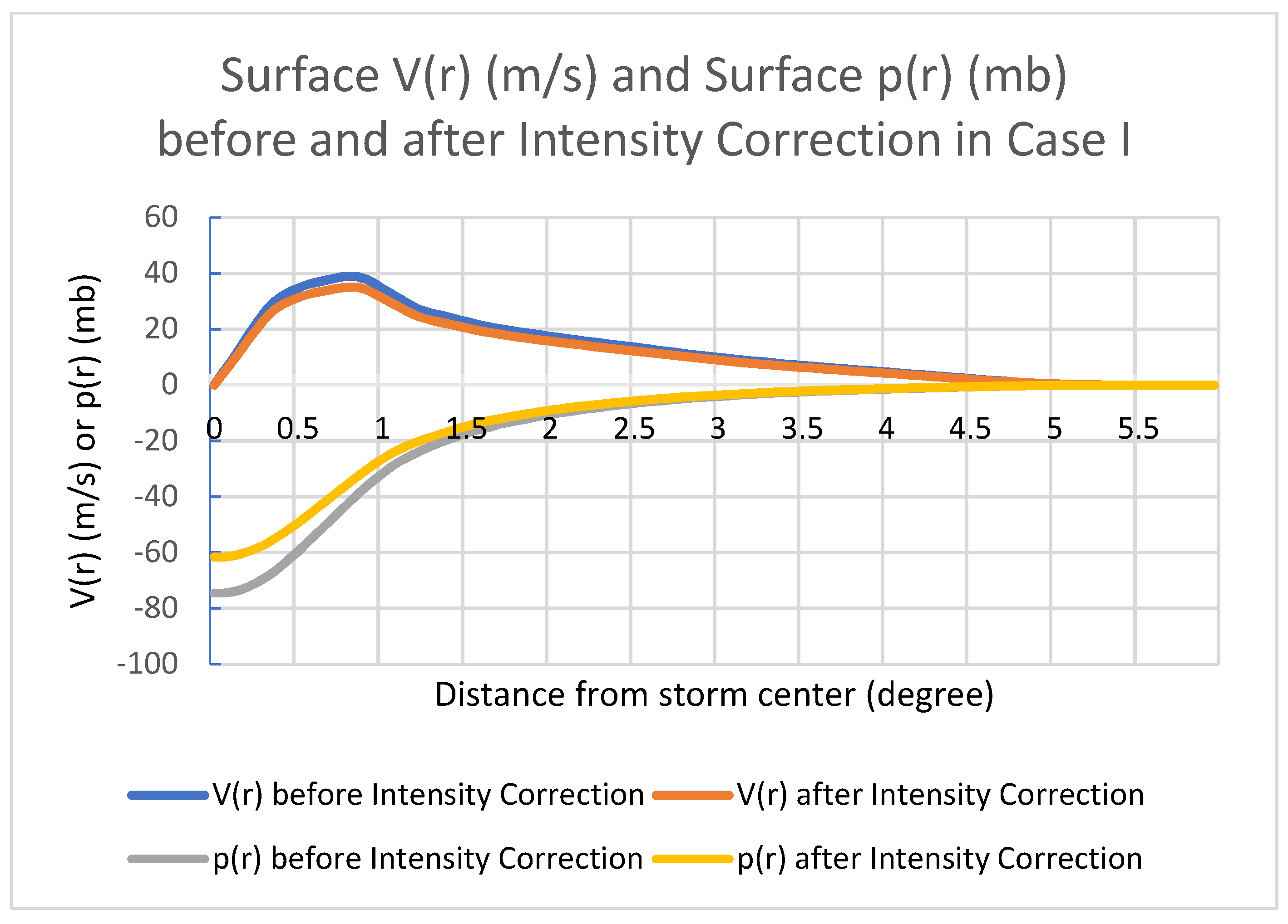
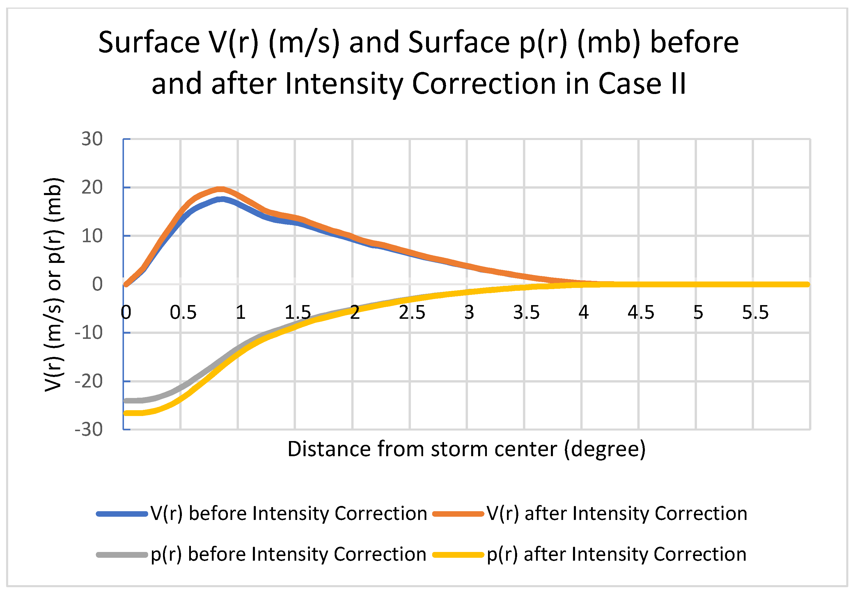
3.3. Storm Intensity Correction

The storm intensity correction was first presented at the American Meteorological Society (AMS) 26th Conference on Hurricane and Tropical Meteorology [17], and tested in the GFDL hurricane model. Generally speaking, the storm in the background field has a different maximum wind speed compared to the observed storm. We need to correct the storm intensity based on the observations. In order to match the observed wind speed, corrections can be large in some cases. In the presence of strong nonlinearity in the hurricane area, we need to use dynamic constraints to correct other variables. Storm intensity correction and the adjustment of other variables will be discussed in detail in the following subsections.

3.3.1. Computation of the Intensity Correction factor β

Let us consider the general formulation in the traditional x, y, and z coordinates. First, we add the vortex back into the environment field after the grid stretching, i.e.:

$$u_1^{*}=\overline{u}+u_1$$

(33)

$$v_1^{*}=\overline{v}+v_1$$

(34)

where $u_1^{*}$ and $v_1^{*}$ are the new background horizontal velocity (environmental field + size corrected vortex). Let $u_2$ and $v_2$ be the vortex horizontal velocity to be added to the background fields. We define:

$$F_1=\sqrt{{\left(u_1^{*}+u_2\right)}^2+{\left(v_1^{*}+v_2\right)}^2}$$

(35)

and:

$$F_2=\sqrt{{\left(u_1^{*}+\beta u_2\right)}^2+{\left(v_1^{*}+\beta v_2\right)}^2}$$

(36)

where $F_1$ is the wind speed at the lowest model level if we simply add a vortex to the background field, and $F_2$ is the new wind speed at the lowest model level after the intensity correction. We consider two cases below.

Case I: $F_1$ is larger than the observed maximum wind speed. We choose $u_2=u_1$ and $v_2=v_1$ to be the vortex horizontal wind components from the previous cycle’s 6-h forecast after grid stretching (this vortex is exactly the same as the vortex we added to the environmental field. We call it vortex #1, which contains both the axisymmetric and asymmetric parts of the vortex).

Case II: $F_1$ is smaller than the observed maximum wind speed. We choose $u_2$ and $v_2$ to be an axisymmetric bogus vortex (vortex #2) which has the observed storm size (radius of maximum wind and ROCI). This bogus vortex is created from a composite storm as discussed in Section 4.

In Case I, we assume that the maximum wind speed for $F_1$ and $F_2$ are at the same model grid point. To find β, we first locate the model grid point where $F_1$ is at its maximum. Let us denote the wind components at this model grid point by $u_1^m$, $v_1^m$, $u_2^m$, and $v_2^m$ (for convenience, we drop the superscript m), so that:

$${\left(u_1^{*}+\beta u_2\right)}^2+{\left(v_1^{*}+\beta v_2\right)}^2=v_{obs}^2,$$

(37)

where $v_{obs}$ is the 10 m observed wind converted to the first model level. Solving for β, we have:

$$\beta =\frac{(-u_1^{*}{u}_2-v_1^{*}{v}_2+\sqrt{v_{obs}^2\left(u_2^2+v_2^2\right)-{\left(u_1^{*}{v}_2-v_1^{*}{u}_2\right)}^2}}{\left(u_2^2+v_2^2\right)},$$

(38)

The procedure to correct wind speed is as follows. First, we calculate the maximum wind speed from Equation (35) by adding the vortex into the environmental fields. If the maximum of $F_1$ is larger than the observed wind speed, we classify it as Case I and calculate the value of β. If the maximum of $F_1$ is smaller than the observed wind speed, we classify it as Case II. The reason we classify it as Case II is that we do not want to amplify the asymmetric part of the storm (amplifying it may negatively affect the track forecasts).

In Case II, iterations may be needed if the storm size has large differences between vortex #1 and vortex #2. We first calculate β as in Case I, and look for the new grid point where F2 reaches its maximum value. We use the variables at this new grid point to calculate β again. This new β will be used to calculate F2. This procedure will be repeated, and β converges in about three iterations.

In summary for Case II, first insert the original vortex into the environmental fields after the storm size correction, and then add a small portion of a bogus storm. The bogus storm portion is calculated from Equation (38). Finally, the new vortex 3D wind field becomes:

$$u\left(x,y,z\right)=u_1^{*}\left(x,y,z\right)+\beta u_2\left(x,y,z\right),$$

(39)

$$v\left(x,y,z\right)=v_1^{*}\left(x,y,z\right)+\beta v_2\left(x,y,z\right),$$

(40)

where $\beta$ is small.

In Case I, we can rewrite Equations (39) and (40) into:

$$u\left(x,y,z\right)=\overline{u}\left(x,y,z\right)+\left(1+\beta \right)u_1\left(x,y,z\right),$$

(41)

$$v\left(x,y,z\right)=\overline{v}\left(x,y,z\right)+\left(1+\beta \right)v_1\left(x,y,z\right),$$

(42)

From the composite vortex, we have the full flow dependent correlation of the other fields (such as the surface pressure, 3D temperature and moisture fields), and we can simply multiply all other fields by $\beta$ and add all the small corrections to the background fields. For example, the temperature field can be rewritten into:

$$T\left(x,y,z\right)=T_1^{*}\left(x,y,z\right)+\beta T_2\left(x,y,z\right),$$

(43)

where:

$$T_1^{*}\left(x,y,z\right)=\overline{T}\left(x,y,z\right)+T_1\left(x,y,z\right).$$

(44)

Generally speaking, $\beta$ is small. However, there are a few cases where $\beta$ can be large. As we know, in the presence of strong nonlinearity in the hurricane area, the above additions may have large errors if $\beta$ is large. Therefore, we move further and use dynamic constraints to correct other variables.

3.3.2. Surface Pressure, Temperature, and Moisture Adjustments

As with the storm size correction, we only correct the axisymmetric part of the surface pressure, temperature and moisture fields after the wind correction. In a high-resolution model, generally speaking, the intensity corrections are small (less than 10%). The first guess fields should be close to the observations, so $\beta$ has a small negative value close to 0 in Case I, and $\beta$ has a small positive value close to 0 in Case II. After the wind speed correction, we need to adjust the sea-level pressure, temperature and the water vapor fields as described below (β can be large in the following discussions).

Let v₁ and v₂ represent the average tangential wind speed for vortex #1 and vortex #2. Following the methodology in Section 3.2.1, we define the gradient wind stream function by:

$${\Psi }_1={\int }_{\infty }^r\left(\frac{v_1^2}{r{f}_0}+v_1\right)dr,$$

(45)

and the new gradient wind stream function is:

$${\Psi }^{new}={\int }_{\infty }^r\left[\frac{{\left(v_1+\beta v_2\right)}^2}{r{f}_0}+\left(v_1+\beta v_2\right)\right]dr,$$

(46)

Since $v_2=v_1$ in Case I, the new gradient wind stream function can be rewritten into:

$${\Psi }^{new}={\int }_{\infty }^r\left[\frac{{\left(\left(1+\beta \right)v_1\right)}^2}{r{f}_0}+(1+\beta )v_1\right]dr,$$

(47)

this formula is used in the code.

The new sea-level pressure perturbation is:

$$\Delta p^{new}=\Delta p\frac{{\Psi }^{new}}{\Psi },$$

(48)

where $\Delta p=p_s-\overline{p}$ and $\Delta p^{new}=p_s^{new}-\overline{p}$ are the hurricane sea-level pressure perturbations before and after the adjustment and $\overline{p}$ is the environment sea-level pressure.

The correction of the temperature field is similar to that in Section 3.2.2. If we replace the environment temperature with the background temperature in Equations (19) and (20), we will have a temperature correction similar to Equation (26), that is:

$$T^{*}=T_b+\Gamma \Delta T=T+\left(\Gamma -1\right)\Delta T,$$

(49)

where $\Gamma ={\Psi }^{new}/\Psi$ and $T_b$ is the background temperature before adding vortex #2. T is the temperature after adding vortex #2 and before the surface pressure correction, and ∆T is perturbation temperature for vortex #2.

The corrections of water vapor in both cases are the same as those discussed in Section 3.2.3.

Generally speaking, the corrections are small. The wind speed correction is less than 10%, and storm size correction is limited to 15%. There are few cases in which the intensity correction is large than 10% (in order to match the observed maximum wind speed), since the gradient wind balance is used in the corrections, the results look fine. The storm structures may still have large differences compared to observations even after the correction. However, as the model physics improves, the storm structure will become better.

4. Bogus Vortex Used to Correct Storm Intensity

The bogus vortex discussed here is primarily used to cold-start for strong storms (with observed intensity greater than or equal to 20 ms⁻¹) and to increase the storm intensity when the storm in HWRF 6-h forecast is weaker than that of the observation (see Section 3.3). This is in contrast to previous HWRF implementations, in which a bogus vortex was used in all cold starts. This change significantly improves the track and intensity forecasts in the first 1–3 cycles of a storm.

The bogus vortex is created from a 2D axisymmetric composite vortex generated from a past model forecast. The 2D vortex only needs to be recreated when the model physics has undergone changes that strongly affect the storm structure. We currently have two composite storms, one created in 2007 for strong deep storms, another one created in 2012 for weak storms.

In order to create the 2D vortex, a forecasted storm (over the ocean) with a small size and near axisymmetric structure is selected. The 3D storm is separated from its environmental fields, and the 2D axisymmetric part of the storm is calculated. The 2D vortex includes the hurricane perturbations of the horizontal wind component, temperature, specific humidity and sea-level pressure. This 2D axisymmetric storm is used to create the bogus storms.

To create a bogus storm, the wind profile of the 2D vortex is smoothed until its radius of maximum winds (RMW) or maximum wind speed matches the observed values. Next, the storm size and intensity are corrected following a procedure similar to the cycled system.

The vortex in medium-depth and deep storms receives identical treatment, while the vortex in shallow storms undergoes two final corrections: the vortex top is set to 400 hPa and the warm core structures are removed (i.e., set the temperature perturbation of the composite storm to be zero).

5. Implementation in the HWRF Model

For simplicity, vortex relocation, size and intensity corrections are performed on a uniform high resolution domain. The domain needs to cover the entire storm area before and after the vortex relocation and size correction. In the HWRF vortex initialization, a domain of size 30 × 30 degrees is used (a large domain requires more memory). For models with multiple nests, data from the parent and nest domains need to be merged to form a single domain.

5.1. Merge Data from Parent and Nests to a Single Domain

In the HWRF vortex initialization, a 30 × 30 degree high-resolution domain (we call it a 3× domain) is created first. The creation of this 3× domain is done exactly the same way the innermost nest (highest resolution) is created, but with a different domain size. After the domain is created, we interpolate the data from the model parent and nests to this new domain, starting with the parent, then the first and second nests. The data in the overlapped regions are replaced by higher resolution data as the interpolation is carried out from parent to nests.

For the data interpolation, first we need to define the hybrid coordinate for the 3× domain (using topography and mean sea-level pressure). Then we interpolate the data from the model grids to the new 3× grids using localized vertical interpolation and E-grid to E-grid horizontal interpolation. The following is a summary of the interpolation used in HWRF.

Consider a new grid point with pressure P (target point) (see Appendix B):

-

Find the surrounding four grid points 1, 2, 3, and 4 (source points);

-

Vertically interpolate data (U, V, T, r) at the four grid points 1, 2, 3, and 4 onto the constant pressure P level (the same pressure level as the target point);

-

Horizontally interpolate the new data at level P from the surrounding four points to the target grid point (E-grid to E-grid interpolation).

This kind of data interpolation, though complicated, carries accurate information from the old grids to the new grids.

5.2. Separation of the Vortex from Its Environment

The code is modified from the GFDL model code, and the procedure is the same as that used in the GFDL model [10,15]. Following [15], the data smoothing is performed on a 40 × 40 degree domain with 1 degree grid resolution. Unlike the GFDL procedure where the storm center is calculated based on the tangential wind, the storm center here is read in from the GFS or HWRF tracker output. The vortex separation procedure is described as follows.

(1)

Interpolate parent data onto a 40 × 40 degree domain with 1 degree resolution, and convert the data to constant pressure levels. Then interpolate data from the 3× domain to this 40 × 40 degree domain, and replace the data in the overlapping area with data from the 3× domain.

(2)

As in the GFDL model, the filter domain is defined from the original wind components at the model level closest to sigma = 0.85. The radius of the filter domain is limited at 1.2 times ROCI, and is always smaller than 11 degrees.

(3)

Separate the vortex from its environment on 1 degree resolution grids using the GFDL method.

(4)

Interpolate the environmental field to the original 3 km resolution (3× domain) only for the grids inside the filter domain.

(5)

Subtract the new 3× domain data (environmental fields) from its original data to obtain the high resolution vortex. The vortex is stored at (2N + 1) constant pressure levels, and the environmental fields of the 3× domain are still on hybrid vertical grids. After the vortex separation, the surface pressure is changed in the hurricane area, so a new vertical coordinate needs to be defined, and all the fields need to interpolate to the new coordinate.

For a cold start, the GFDL filter is applied to GFS analysis fields to create the large-scale environmental fields. For a warm start, the GFDL filter is applied to both the GFS analysis fields and 6-h HWRF forecast.

After vortex separation, we smooth the vortex field to avoid large wind speeds due to the boundary layer turbulence (which does not represent the vortex strength). We also calculate the axisymmetric vortex for use in temperature and water vapor field adjustments after the storm size and wind speed correction.

5.3. Vortex Relocation and Size Correction

In storm relocation, we simply move the vortex based on the model forecast storm center and the observed storm center. In the following, we mainly focus on explaining some details about the storm size correction. The storm size correction needs two parameters, namely, the radius of max wind (RMW) and radius of the 34 knot wind (R34) (or radius of the outmost closed isobar ROCI). To search for the maximum wind speed (or RMW) from the 6-h model forecast field, we first define the search area. Let $r_o$ be the observed radius (in degree of latitude/longitude) of the max wind speed, and the search area R is defined by:

$$R=\min \left(3.5,\max \left(2.5r_o, 2.0\right)\right)$$

(50)

Let $r_m$ be the radius of the maximum surface wind speed from the model 6-h forecast, so the target of the size correction is defined by:

$$r_t=0.5\left(r_m+r_o\right)$$

(51)

The correction limit is set to be 15% of r_m. The correction for the second parameter R34 or ROCI is also limited to 15% of the model value.

To calculate R34, we scale the storm intensity to match the observations, and search the model grid for where the wind speed equals/exceeds 34 knots to find the distance from ROCI to the storm center for each of the four quadrants. The maximum distance from each quadrant is defined as R34 in that quadrant. The maximum R34 from the four quadrants is used for the storm size correction.

For weak storms (where R34 does not exist), ROCI is used for the storm size correction. However, the calculation of ROCI has large uncertainty from the model output. Therefore, ROCI is used only as a reference in storm size correction.

Once we define the 6-h model variables r_m and R_m (or ROCI), we can compress/stretch the model grid to the target values, and calculate the coefficients a and b from Equation (5), or compress/stretch the function f(i,j) from Equation (6).

The storm relocation and storm size correction are done simultaneously in the code:

hlat(i,j) = (hlat(i,j) − clat_fcst)* f(i,j) + clat_obs,

(52)

hlon(i,j) = (hlon(i,j) − clon_fcst)* f(i,j) + clon_obs,

(53)

vlat(i,j) = (vlat(i,j) − clat_fcst)* f(i,j) + clat_obs,

(54)

vlon(i,j) = (vlon(i,j) − clon_fcst)* f(i,j) + clon_obs,

(55)

Here, f(i,j) is the stretching factor. (hlon(i,j), hlat(i,j)) and (vlon(i,j), vlat(i,j)) are the longitude and latitude of the model h-points and v-points, respectively. (clon_fcst, clat_fcst) and (clon_obs, clat_obs) are the forecast storm center and the observed storm center, respectively. After the grids are compressed or stretched, we need to interpolate the data back to the original model grids. The storm size correction is more complicated than the simple description here due to the E-grid to E-grid interpolation (see discussion in Section 5.1).

5.4. Surface Pressure, Temperature, and Mixing Ratio Correction

After the model grid compression or stretching, we need to correct the surface pressure, temperature and moisture fields as discussed in Section 3.2. The correction only applies to the axisymmetric part of the storm. We first calculate the gradient wind stream function before and after the grids are stretched.

Before the grids are stretched, we set:

$$\mathrm{Radius}: R_{k1}\left(n\right)=r\left(n\right),$$

(56)

$$\mathrm{Tan}\mathrm{gential} \mathrm{wind} \mathrm{speed}: W_{k1}\left(n\right)=U\_S\left(n\right),$$

(57)

where r(n) is in meters, and U_S(n) is in m/s, and n represents the grid in cylindrical coordinates.

After the grids are stretched, we have:

$$\mathrm{Radius}: R_{k2}\left(n\right)=\left(a·r\left(n\right)+0.5·b·r^2\left(n\right)\right),$$

(58)

$$\mathrm{Tan}\mathrm{gential} \mathrm{wind} \mathrm{speed}: W_{k2}\left(n\right)=U\_S\left(n\right),$$

(59)

The gradient wind stream functions are calculated by:

$${\Psi }_1\left(n\right)={\displaystyle \sum _{i=\infty }^n}\left(\frac{W_{k1}\left(i\right)}{R_{k1}\left(i\right)}+f_0\right)·W_{k1}\left(i\right)$$

(60)

and:

$${\Psi }_2\left(m\right)={\displaystyle \sum _{i=\infty }^m}\left(\frac{W_{k2}\left(i\right)}{R_{k2}\left(i\right)}+f_0\right)·W_{k2}\left(i\right)$$

(61)

where $f_0=2.7292·{10}^{-5}·\sin \left(clat\_obs·\frac{\pi }{180}\right)$ is the Coriolis parameter.

After the calculation of ${\Psi }_2\left(m\right)$, we need to interpolate the data back to the original grid r(n). Let’s denote the new data by ${\Psi }_2\left(n\right)$, so we can define the correction function by:

$$\zeta \left(n\right)=\frac{{\Psi }_2\left(n\right)}{{\Psi }_1\left(n\right)}$$

(62)

Then the increment for surface pressure is:

$$\Delta p\left(n\right)=\left(\zeta \left(n\right)-1\right)·SLP\_S\left(n\right)$$

(63)

The increment for temperature field is:

$$\Delta T\left(n, k\right)=\left(\zeta \left(n\right)-1\right)·T\_S\left(n, k\right)$$

(64)

The increments for sea-level pressure and temperature fields in cylindrical coordinates are converted to Cartesian coordinates before adding them to the vortex.

The mixing ratio is calculated after the vortex temperature is added to the background temperature fields. The calculation of the mixing ratio uses Equations (30) and (32).

After the corrections of surface pressure, mixing ratio and temperature components, we need to redefine the vertical coordinate. All data are interpolated to the new coordinate.

5.5. Intensity Correction

As discussed before, the intensity correction is separated into two cases. When a storm in the 6-h forecast is stronger than the observation, we multiply the 3D wind field by a factor β (β < 1), and adjust the surface pressure, temperature and mixing ratio fields as discussed in Section 3.3 to the vortex before inserting it into the environmental field.

When storm in the 6-h forecast is weaker than the observation, we first insert the 6-h vortex into the environment field after the storm size correction to form a new background field. Then we add a small fraction of a composite storm to the new background field to match the observed storm intensity. The composite storm undergoes a storm size and intensity correction before it is added into the new background field. The corrections for the thermodynamic fields are discussed in Section 3.3.

6. Test Results and Some Real-Time Runs

We have performed large number of sensitivity experiments to adjust the algorithm and parameters before the initialization was implemented in operations. Generally speaking, the HWRF track statistics have the comparable forecast skills as those of the operational GFS model, and slightly degraded in the longer-range forecast (3–5 days) due to lateral boundary conditions of the regional model. The intensity forecast skills are better than that of GFS except for storms in a strong shear environment.

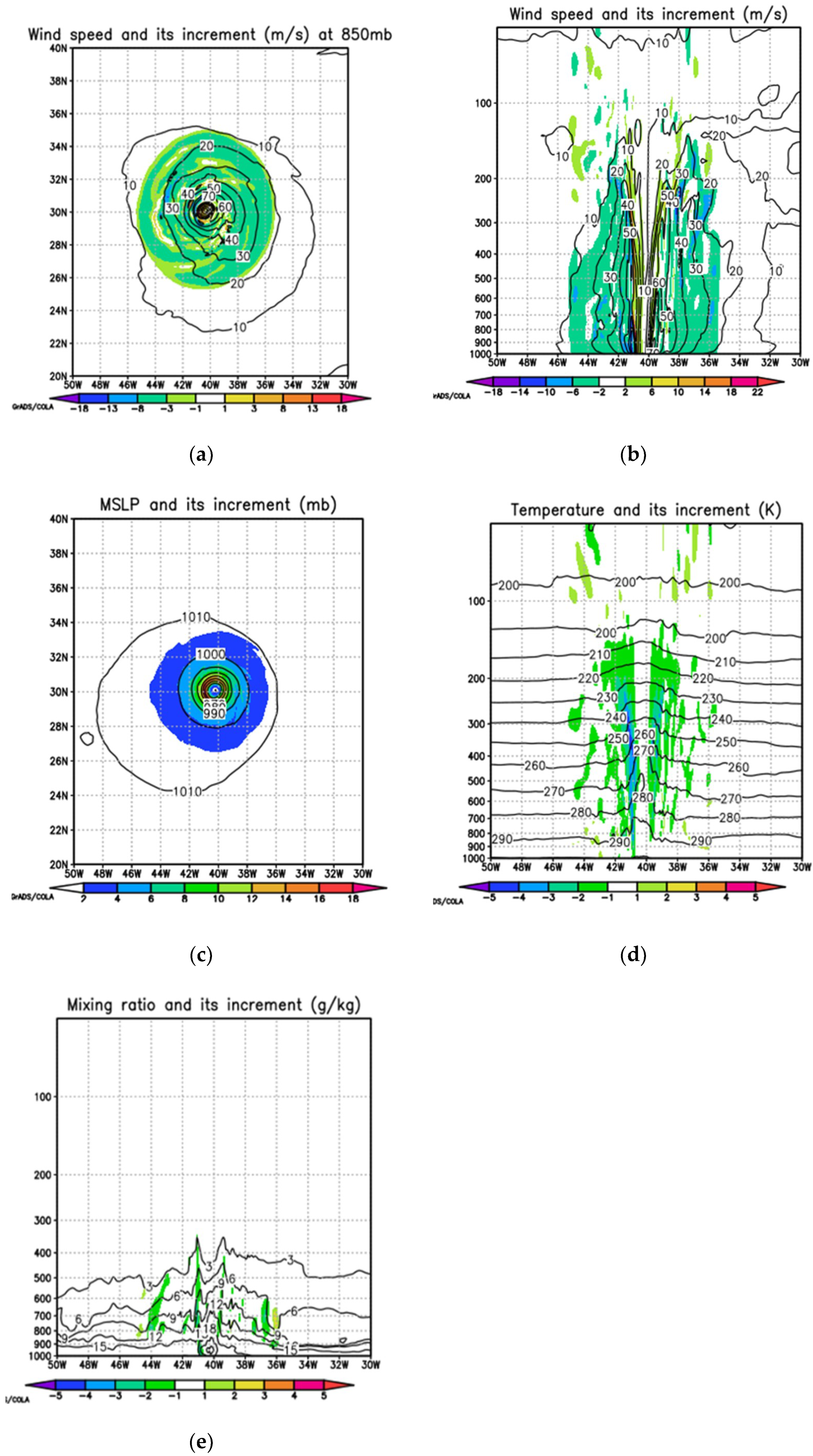
6.1. Impacts of Background Vortex Initialization

We show some examples of the background vortex and the impacts of the VI in this section. The first example is the impact of storm size correction. For TC Lorenzo (13 L), the background vortex comes from the cycle at 1800 UTC 29 September 2019. The background vortex initialization includes three steps: relocation, size correction and intensity correction. In the vortex relocation step, we simply move the background vortex to the observed location without altering the vortex structure and intensity (not shown here).

Figure 1 shows the impacts of the storm size correction on the storm azimuthally averaged surface tangential wind speed V(r) and the averaged MSLP perturbation p(r) (environment fields have been removed). The storm size is reduced by ~10% (a ≈ 0.9, and b = 0 in Equation (2)) during the VI. Due to the storm size reduction, the wind speed is smaller when r ≥ 0.8° (where r ≈ 0.8° is the radius of the maximum V(r)) and larger when r < 0.8° compared to the wind speed of the original vortex (orange line vs. blue line). Since MSLP is an integrated quantity, as a result of the storm size change, the differences of the MSLP perturbations (differences between yellow line and gray line) gradually increase as we integrate from storm edge to r ≈ 0.8°, and gradually decrease when we integrate from r ≈ 0.8° to the storm center.

Figure 2 shows the background fields and their related increments after storm size correction. The initialization increment after the storm size correction spreads all the way to the edge of the storm, and has large values whenever the radial gradient of the tangential wind speed is large (Figure 2a–e). In contrast, the initialization increments after the intensity correction are mainly located near the storm center where the wind speed is large (Figure 3, Figure 4, Figure 5 and Figure 6).

The next two examples are for intensity correction. For intensity correction in Case I, we use the same background vortex as the one used in the storm size correction. The storm wind speed is reduced by ~10% (β ≈ 0.9) during the VI. Figure 3 shows the impacts on the storm azimuthally averaged surface tangential wind speed V(r) and the azimuthally averaged MSLP perturbation p(r). Due to the reduction of V(r) (orange line vs. blue line) in the VI, the MSLP perturbation at the storm center increased by roughly 18 mb. For intensity correction in Case II, the background vortex comes from TC Lorenzo (13 L) of the cycle at 1200 UTC 25 September 2019. Figure 4 shows the impacts of the storm intensity correction in Case II, where the maximum surface wind speed increased by ~10%, and the storm MSLP perturbation decreased by ~4.7 mb at the storm center.

Figure 5 and Figure 6 show the background fields and their related increments after storm intensity corrections in Case I and Case II, respectively. The storm intensity correction is ~10% in both cases. As mentioned before, the initialization increments after the intensity correction are mainly located near the storm center where the wind speed is large (Figure 3, Figure 4, Figure 5 and Figure 6). The increments of the storm intensity correction in Case I is close related to the background vortex, whereas the increments of the storm intensity correction in Case II are very similar to the bogus vortex used during the intensity correction.

As discussed in Section 3, the surface pressure is corrected right after the storm size or storm wind correction. The surface pressure correction directly affects the upper level temperature and the mixing ratio increments. Figure 2d, Figure 5d, and Figure 6d give the vertical cross section of temperature increments. The temperature increments are small for the storm intensity correction compared to those of the storm size correction. The same is true for the mixing ratio increments (Figure 2e, Figure 5e, and Figure 6e).

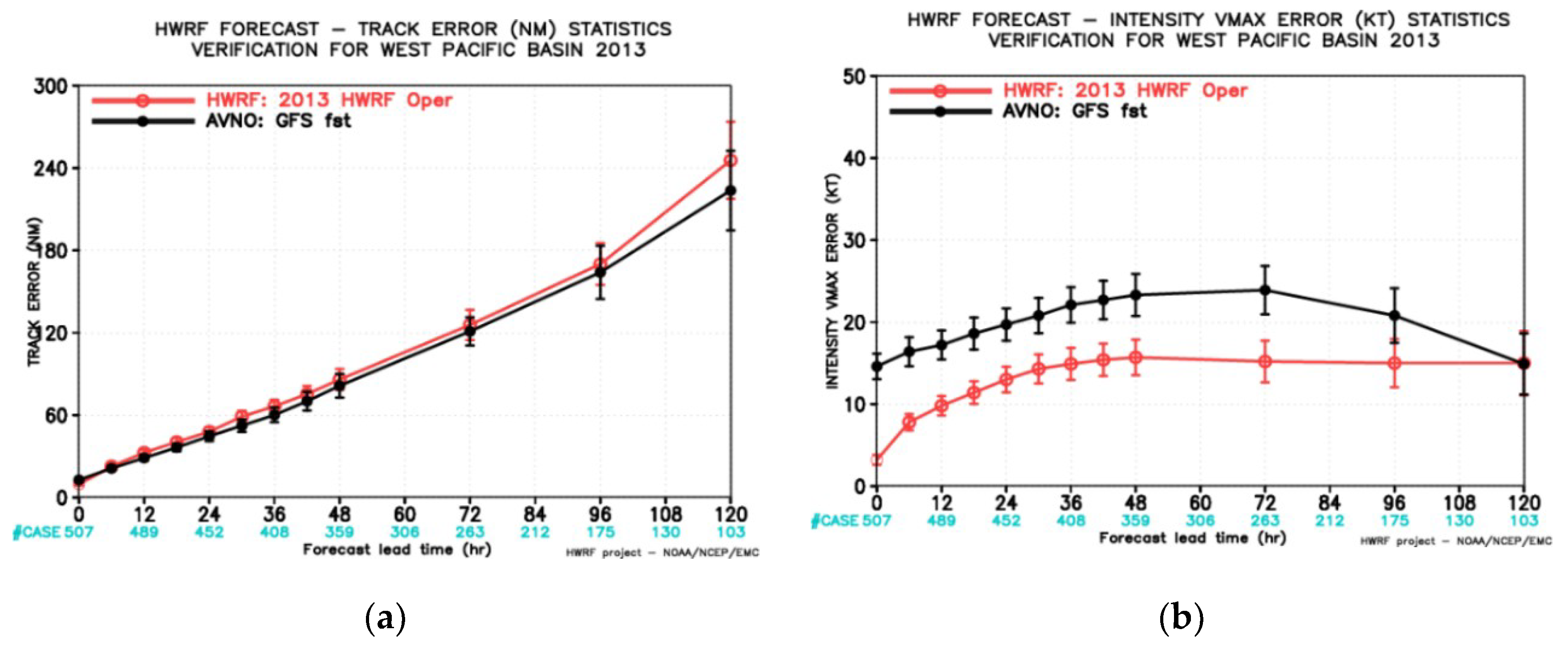
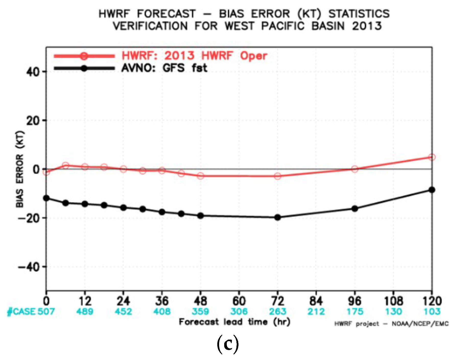
6.2. Some Results from 2013 Real-Time Runs

The purpose of his paper is to document a technique of the vortex initialization in the operational hurricane models. However, it is still good to show the positive impact of the VI technique on the operational HWRF real-time forecasts. The vortex initialization discussed here has been implemented in the operational HWRF model in the Atlantic basin since 2007 and in the West Pacific basin in 2012. Pre-implementation test runs for the 2010–2012 seasons show the track forecast has a comparable skill as that of GFS, and the intensity forecasts are better than those the statistical models. Here, we show the statistics for all named Western Pacific storms in the 2013 hurricane season (no data assimilation in HWRF for West Pacific storms). Figure 7a shows the track forecast is close to GFS forecast skill. The initial intensity in HWRF is significantly better compared to those in GFS (Figure 7b), and the intensity forecast in HWRF does not show spin-up/spin-down problems. The bias for the intensity forecast is close to zero, whereas the global model has a very large negative bias (Figure 7c).

7. Discussion and Conclusions

We have described a vortex initialization (i.e., background vortex initialization in the operational community) method to initialize tropical cyclones in numerical models. This method is a natural extension of the vortex relocation technique. The vortex initialization technique presented here uses TCVital data to improve the background vortex fields. Other data (such as the airborne radar observations) can be added through traditional data assimilation such as the GSI to further improve storm structure and its environment flow. There is no conflict between the vortex initialization presented here and traditional data assimilation. The vortex initialization is simple and computationally efficient. It is currently used in the operational HWRF model (reference: DTC HWRF Scientific Document, 2012), and has also been adapted for the operational HMON.

We would like to mention that the storm intensity correction is, in fact, a form of data analysis. The observation data used in this process is the surface maximum wind speed (single-point observation data in TCVital), and the background error correlations are flow dependent and based on the model predicted storm structure. The storm structure used for the background error correlation is the 6 h forecasted vortex from previous cycle when storm intensity is overpredicted, and is the composite vortex when storm intensity is underpredicted (or the forecast cycle is a cold start cycle). In HWRF, the previous 6-h forecasted storm structure is not reliable if the background vortex is weak, and therefore an axisymmetric composite vortex from old model forecasts is employed to correct the storm intensity.

The intensity forecasts from the HWRF model tend to over-intensify in the strong shear environment. Although this problem is mostly related to the model physics, better initial vortex structure can improve the model intensity forecasts. Currently, data assimilation in the hurricane inner core area remains a challenge although there are some progresses have been made. The major reason is that there are large differences between the observation data and the background vortex fields. Since 2013, Airborne Doppler radar data has been assimilated in the HWRF vortex initialization although they are only available when the NOAA’s P-3 reconnaissance flights are deployed. The abundant satellite data in the inner core area may be used in the HWRF vortex initialization in the future either through data assimilation or empirical methods.

References

1. Leslie, L.M.; Holland, G.J. On the bogussing of tropical cyclones in numerical models: A comparison of vortex profiles. Meteorol. Atmos. Phys. 1995, 56, 101–110. [Google Scholar] [CrossRef]
2. Davidson, N.E.; Weber, H.C. The BMRC high-resolution tropical cyclone prediction system: TC-LAPS. Mon. Weather Rev. 2000, 128, 1245–1265. [Google Scholar] [CrossRef]
3. Kwon, I.-H.; Cheong, H.-B. Tropical cyclone initialization with a spherical high-order filter and an idealized three-dimensional bogus vortex. Mon. Weather Rev. 2010, 138, 1344–1367. [Google Scholar] [CrossRef]
4. Rappin, E.D.; Nolan, D.S.; Majumdar, S.J. A highly configurable vortex initialization method for tropical cyclones. Mon. Weather Rev. 2013, 141, 3556–3575. [Google Scholar] [CrossRef]
5. Lord, S.J. A bogussing system for vortex circulations in the National Meteorological Center Global Forecast Model. Preprints. In 19th Conference on Hurricanes and Tropical Meteorology; American Meteor Society: Miami, FL, USA, 1991; pp. 328–330. [Google Scholar]
6. Fiorino, M.; Elsberry, R.L. Some aspects of vortex structure related to tropical cyclone motion. J. Atmos. Sci. 1989, 46, 975–990. [Google Scholar] [CrossRef] [Green Version]
7. Goerss, J.; Jeffries, R. Assimilation of synthetic tropical cyclone observations into the Navy Operational Global Atmospheric Prediction System. Weather Forecast. 1994, 9, 557–576. [Google Scholar] [CrossRef] [Green Version]
8. Radford, A.M. Forecasting the movement of tropical cyclones at the Met. Off. Meteorol. Appl. 1994, 1, 355–363. [Google Scholar] [CrossRef]
9. Heming, J.T.; Chan, J.C.-L.; Radford, A.M. A new scheme for the initialization of tropical cyclones in the UK Meteorological Office global model. Meteorol. Appl. 1995, 2, 171–184. [Google Scholar] [CrossRef]
10. Kurihara, Y.; Bender, M.A.; Tuleya, R.E.; Ross, R.J. Prediction experiments of Hurricane Gloria (1985) using a multiply nested movable mesh model. Mon. Weather Rev. 1990, 118, 2185–2198. [Google Scholar] [CrossRef] [Green Version]
11. Pu, Z.; Braun, S.A. Evaluation of bogus vortex techniques with four-dimensional variational data assimilation. Mon. Weather Rev. 2001, 129, 2023–2039. [Google Scholar] [CrossRef]
12. Cha, D.-H.; Wang, Y. A dynamical initialization scheme for real-time forecasts of tropical cyclones using the WRF model. Mon. Weather Rev. 2013, 141, 964–986. [Google Scholar] [CrossRef]
13. Hendricks, E.A.; Peng, M.S.; Li, T.; Ge, X. Performance of a dynamic initialization scheme in the Coupled Ocean– Atmosphere Mesoscale Prediction System for Tropical Cyclones (COAMPS-TC). Weather Forecast. 2011, 26, 650–663. [Google Scholar] [CrossRef]
14. Gall, R.; Franklin, J.; Marks, F.D.; Rappaport, E.N.; Toepfer, F. The Hurricane Forecast Improvement Project. Bull. Am. Meteorol. Soc. 2013, 94, 329–343. [Google Scholar] [CrossRef]
15. Kurihara, Y.; Bender, M.; Tuleya, R.; Ross, R. Improvements in the GFDL Hurricane Prediction System. Mon. Weather Rev. 1995, 123, 2791–2801. [Google Scholar] [CrossRef] [Green Version]
16. Kleist, D.T.; Parrish, D.F.; Derber, J.C.; Treadon, R.; Wu, W.-S.; Lord, S.J. Introduction of the GSI into the NCEP Global Data Assimilation System. Weather Forecast. 2009, 24, 1691–1705. [Google Scholar] [CrossRef] [Green Version]
17. Liu, Q.; Surgi, N.; Lord, S.; Wu, W.-S.; Parrish, S.; Gopalakrishnan, S.; Waldrop, J.; Gamache, J. Hurricane Initialization in HWRF Model, Preprints. In Proceedings of the 27th Conference on Hurricanes and Tropical Meteorology, Monterey, CA, USA, 24–28 April 2006. [Google Scholar]
18. Liu, Q.; Marchok, T.; Pan, H.-L.; Bender, M.; Lord, S. Improvements in Hurricane Initialization and Forecasting at NCEP with Global and Regional (GFDL) Models; NCEP Office Note 472; NCEP/NOAA/DOC: Silver Spring, MD, USA, 2000.
19. Liu, Q.; Lord, S.; Surgi, N.; Pan, H.L.; Marchok, T.; Tuleya, R.; Bender, M. Hurricane Initialization in High Resolution Models. In Proceedings of the 26th AMS Conference on Hurricanes and Tropical Meteorology, Miami, FL, USA, 2–7 May 2004. [Google Scholar]
20. Liu, Q.; Lord, S.; Surgi, N.; Zhu., Y.; Wobus, R.; Toth, Z.; Marchok, T. Hurricane relocation in global ensemble forecast system. Preprints. In 27th Conference on Hurricanes and Tropical Meteorology; American Meteor Society: Monterey, CA, USA, 2006; Volume 5, p. 13. [Google Scholar]
21. Tong, M.; Sippel, J.A.; Tallapragada, V.; Liu, E.; Kieu, C.; Kwon, I.H.; Wang, W.; Liu, Q.; Ling, Y.; Zhang, B. Impact of assimilating aircraft reconnaissance observations on tropical cyclone initialization and prediction using operational HWRF and GSI ensemble–variational hybrid data assimilation. Mon. Weather Rev. 2018, 146, 4155–4177. [Google Scholar] [CrossRef]
22. Gopalakrishnan, S.G.; Goldenberg, S.; Quirino, T.; Marks, F.; Zhang, X.; Yeh, K.-S.; Atlas, R.; Tallapragada, V. Towards improving high-resolution numerical hurricane forecasting: Influence of model horizontal grid resolution, initialization, and physics. Weather Forecast. 2012, 27, 647–666. [Google Scholar] [CrossRef]
23. Schubert, W.H.; Hack, J.J. Transformed Eliassen balanced vortex model. J. Atmos. Sci. 1983, 40, 1571–1583. [Google Scholar] [CrossRef] [Green Version]
24. Bolton, D. The computation of equivalent potential temperature. Mon. Weather Rev. 1980, 108, 1046–1053. [Google Scholar] [CrossRef] [Green Version]
25. Janjic, Z. A nonhydrostatic model based on a new approach. Meteorol. Atmos. Phys. 2003, 82, 271–285. [Google Scholar] [CrossRef]
Figure 1. Impacts of the storm size correction. The storm size is reduced by ~10%. V(r) is the azimuthally averaged storm surface tangential wind speed (m/s), p(r) is the azimuthally-averaged storm MSLP perturbation (mb). The blue line and the orange line are the V(r) before and after the size correction, respectively. The gray line and the yellow line are p(r) before and after the size correction, respectively.
Atmosphere 11 00968 g001
Figure 2. (ae) The background fields and their increments after storm size corrections. (a) The background horizontal wind speed (m/s) (contour) and its initialization increment (m/s) (shaded) at 850 mb; (b) vertical cross-section of the background horizontal wind speed (m/s) (contour) and its increment (m/s) (shaded) at the latitude 30° N (storm center); (c) mean sea-level pressure (mb) (contour) and its increment (mb) (shaded); (d) vertical cross-section of the background temperature (K) (contour) and its increment (K) (shaded) at the latitude 30° N; (e) vertical cross-section of the background mixing ratio (g/kg) (contour) and its increment (g/kg) (shaded) at the latitude 30° N.
Atmosphere 11 00968 g002
Figure 3. Same as Figure 1 but for storm intensity correction in Case I (wind speed reduced by ~10%).
Atmosphere 11 00968 g003
Figure 4. Same as Figure 1 but for storm intensity correction in Case II (maximum surface wind speed increased by ~10%).
Atmosphere 11 00968 g004
Figure 5. (ae): Same as Figure 2 but after storm intensity corrections in Case I (storm center is located at latitude 30° N).
Atmosphere 11 00968 g005aAtmosphere 11 00968 g005b
Figure 6. (ae) Same as Figure 2 but after storm intensity corrections in Case II (storm center is located at latitude 13.4° N).
Atmosphere 11 00968 g006aAtmosphere 11 00968 g006b
Figure 7. (ac). Statistics of the typhoon forecasts in Western Pacific basin in 2013 hurricane season real-time run. Red line is for HWRF, black line is for GFS. (a): track forecasts; (b): intensity forecasts; (c): Bias of intensity forecasts.
Atmosphere 11 00968 g007aAtmosphere 11 00968 g007b