Abstract
The spatio–temporal evolution of the Pacific blocking frequency (PBF) that is based on a two–dimensional blocking index is investigated during the recent 40–winter (1979/80–2018/19) months (December–January–February). It is found that maximum PBF appears in January within the key area of 140° E–160° W, 50°–70° N. The key–area Pacific blocking in January is more active during the first (1980–1988) and the third (2009–2019) periods than during the second period (1989–2008). There is a positive 500 hPa–geopotential height (Z500) anomaly over the mid–latitude Pacific and a negative one over the high latitude area between the first two periods (second minus first). This pattern can cause an anomalous westerly circulation over the mid–high Pacific sector, which indicates a weakening of the Pacific blocking activity during the second period. This connects to a positive two–meter air temperature (T2m) anomaly over the northeastern Asia and mid–western Pacific, and a negative one over the high–latitude area. The difference of Z500 between the third and the second periods (third minus first) is opposite to that between the second and the first periods, which leads to more Pacific blocking events during the third period. This is related to a positive T2m anomaly over the high–latitude area and a negative one over the mid–latitude area of Asia and the western Pacific. Furthermore, the correlation coefficient between the variables (Z500, T2m, 200 hPa–zonal wind) and the key–area PBF confirms the above results.
1. Introduction
Atmosphere blocking is a result of a meridional–type flow interrupting the normal zonal flow at mid- and high- latitudes [1]. Blocking activities are often accompanied by a widespread adjustment of circulation, which may lead to extreme weather during winter or summer time [2,3]. Blocking plays a crucial role in cold wave and extreme cold surface air temperature during winter time and, in heatwave and drought events during summer time, causes serious economic losses [3,4,5,6]. For example, freezing rain and snowstorm in South China during January 2008 is largely influenced by blocking high occurring over the Ural Mountains, which affected the life of more than 100 million people [5]. Therefore, previous studies paid attention to the effect of blocking by different methods for detecting blocking [2,3,7,8,9].
Rex [1] defined blocking action using early upper–air data. A one–dimensional (1D) blocking index (hereinafter TM90) was constructed based on searching the reversal of the meridional gradient of 500 hPa–geopotential height in order to identify blocking conveniently [10]. Scherrer et al. [11] developed TM90 to a two–dimensional (2D) domain (hereinafter S06). Davini et al. [12] improved the 2D blocking index (hereinafter D12) based on S06. It is found that high–latitude blocking occurs over Greenland and the Pacific Ocean and mid–latitude blocking occurs over the Euro–Atlantic region [12]. The concept of Rossby wave breaking is linked with blocking events [7,11,12,13]. According to this concept, a new one–dimensional (1D) blocking index (hereinafter PH03) is constructed by Pelly and Hoskins [14]. PH03 is based on the reversal of the potential temperature gradient at two–potential vorticity unit (PVU) surface [14]. However, the major properties of wave breaking are the orientation (cyclonic breaking or anticyclonic breaking) and the relative contribution of air masses (warm–relative intensity or cold–relative intensity) [2]. According to these properties, the 1D index defined by PH03 is extended to a 2D index (hereinafter M13) [7,15]. When compared to D12, M13 is deemed that the influence of the subtropical westerly jet on blocking is weak, leading to no blocking over the subtropics [15]. In addition, there are other differences between the M13 and else blocking index (e.g., TM90, S06, and D12). This blocking index (M13) is symmetrical in the sense that it searches in order to identify the poleward blocking anticyclone and the equatorward cutoff cyclone [15]. This contrasts with the methods (e.g., [10,11,12]) in which there is the other one criterion of strong westerly winds on the poleward side, focusing on only the blocking anticyclone. Thus, the blocking frequency in this study is higher than that in other studies [16,17,18,19,20,21,22,23].
Using these blocking indices, it was found that not only the climatic mean state, but also the systems on different timescales can influence blocking activities, such as El Niño–Southern Oscillation (ENSO), North Atlantic Oscillation (NAO), and Madden–Julian oscillation (MJO) [8,9,11,24]. Because blocking can result in extreme events, it is necessary to understand the spatiotemporal characteristics of blocking in each month, which is helpful in improving the forecast abilities of extreme events. The blocking activities were largely studied by the 1D blocking index (e.g., TM90 and PH03), but the 1D index cannot describe the 2D spatial distribution of the blocking frequency. On the other hand, the studies of statistical analysis about the blocking frequency mainly focused on the interannual or interdecadal variation during the whole winter. However, the blocking frequency is different among different months. Therefore, it is necessary to analyze the blocking frequency in each winter month.
In this study, the 2D blocking index used by M13 is used to analyze the spatial–temporal evolution of the blocking frequency over the Pacific sector during the recent 40–winter (1979/80–2018/19) months (December–January–February, totally 120 months). The remaining part is organized, as follows. Section 2 introduces datasets and methods. In this section, a 2D blocking index is provided. The characteristics of the 2D–distribution of Pacific blocking frequency during winter time (December–January–February, DJF) are analyzed in Section 3. The maximum frequency appears in January, so the space–time features of blocking frequency in January are mainly investigated in this section. Section 4 concludes the main findings.
2. Data and Method
Daily reanalysis data during 1979–2019 with a horizontal resolution of 1.5° × 1.5° provided by the European Centre for Medium–Range Weather Forecasts Interim reanalysis (ERA–Interim, [25]) is used in this study. The variables include 500 hPa–geopotential height Z500, 200 hPa–zonal wind U200, and two meter–surface temperature T2m.
The Northern Hemisphere blocking index used in this study is based on [15], which detects blocking by the average difference of Z500 across a latitude ϕ0, given by:
The lambda means longitude and ϕ0 is varied between 40° N and 75° N. A grid is defined as instantaneous blocking when B is greater than 0. The grid with the B greater than 0 indicates averaged higher pressure to its north and lower pressure to its south [8,9]. Refer to [8] and [15], is set to 30°. Equation (1) is separately applied to two sectors: Pacific sector (120° E–150° W, 40°–75° N) and European sector (21° W–45° E, 40°–75° N), referring to [8] and [15]. The approach of tracking blocking events within each sector is described as follow.
First, local positive maxima of B are found at each day from the defined sector, indicating each blocking center. Second, if a blocking center of the next day is within a 27° (latitude) × 36° (longitude) box, centered at the local maximum of the previous day, this blocking center is considered as the continuation of the blocking event. Otherwise, the beginning of a new event is defined. Besides, the end of a blocking event is also defined when there is no positive continuation B within an area 50% greater than the box, being centered at the maxima of the onset. Third, only the blocking event lasting more than 5 days and the continuous positive B associated with the blocking center are both retained. Finally, a dichotomous index is generated in order to calculate the blocking frequency for each grid. If the criteria of blocking event are satisfied in a grid, a value of 1 is assigned on this grid and, if criteria are not satisfied, a value of 0 is assigned.
Figure 1a shows the longitudinal distribution along 45°–75° N of the blocking frequency associated with 120 winter months. It is clearly seen that there are two peaks, with one located at Pacific region (left shading) and another at European region (right shading). The result is consistent with [8]. The maximum frequency over Pacific sector is about 25%. The 25% means approximately 902 days out of 3610 (the total days in winter) experienced blocking in this longitude. The maximum frequency over Europe is about 6%. Because the usage of different blocking diagnostic methodologies can cause different results [26]. The maximum frequency over Europe in this study is smaller than that in other studies (e.g., [10,20]). The maximum frequency over Europe is much less than that over Pacific sector. We mainly focus on the Pacific blocking. Figure 1b displays the horizontal distribution of the Pacific blocking frequency (PBF) in 120 winter months. The frequency of each grid is the ratio of the total blocking days to the total 3610 days. It is shown that the Pacific blocking mostly occurs at the latitude north of 50° N. The maximum PBF appears over the northern Okhotsk Sea and the northern Asian continent (150°–175° E, 60°–65° N), with a maximum value that exceeds 44%. In addition, the mostly blocking centers approximately locate at 145° E (not shown).
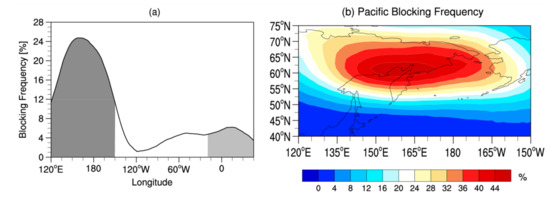
Figure 1.
(a) Blocking frequency (unit: %) as a function of latitude averaged between 45° N and 75° N including Pacific sector (left shading; 120° E–150° W) and European sector (right shading; 21° W–45° E) during boreal winter (December–January–February, DJF); (b) Horizontal distribution of Pacific blocking frequency in DJF.
3. Intraseasonal Variation of the PBF
3.1. Horizontal Distribution
In this subsection, we focus on horizontal evolution of the PBF in individual months. Because the PBF may have different features among DJF, we examine the horizontal distribution of the PBF in these three months, respectively. The statistical result shows that the PBF is 64.1% in 40–yr (1979–2018) December, while the frequency is 72.1% and 67.5% in 40–yr (1980–2019) January and February, respectively. This suggests that the Pacific blocking in January is the most active.
Figure 2 displays the horizontal evolution of the PBF in the three months. The maximum PBF appears over 140° E–170° W, 55°–70° N, with a maximum value of about 36% in December (Figure 2a). The Pacific blocking occurs mostly to the north of the Okhotsk Sea, between 55° N and 65° N, with a maximum frequency of more than 49% in January (Figure 2b). The maximum PBF is about 39% in February (Figure 2c). Figure 2d shows the horizontal distribution of the PBF difference between January and December (former minus latter). As shown, a positive frequency anomaly is located over between 50° N and 65° N. The dotted in Figure 2d means the region exceeding 0.01 significance level. This suggests that the Pacific blocking is more active in January than that in December. Figure 2e shows the horizontal distribution of the PBF difference between January and February. The positive anomaly dominates the whole Pacific region. This suggests that the Pacific blocking in January is also more active than that in February. In addition, Figure 2d,e are repeated by the 20CRV3 reanalysis dataset [27]. Similar patterns and numbers are represented (not shown). This also suggests that the Pacific blocking in January is more active than others. Some studies indicate that the opposite–signed Madden–Julian Oscillation (MJO) heating during phase 7 and 8 have been linked to significant changes in Pacific winter blocking [8,9]. The composite 30–70–day band filtered OLR of phase 7–8 during the three months indicate that the opposite–signed MJO heating in January is stronger than others (not shown). Accordingly, the reason for the more active Pacific blocking in January relative to December and February may be the influence of MJO.
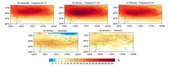
Figure 2.
(a) Horizontal distribution of Pacific blocking frequency (unit: %) in December; (b,c) As in (a), but for January and February, respectively; (d) Difference of the Pacific blocking frequency between (a) and (b); (e) As in (d), but for the difference between (c) and (b). Dotted area indicates the difference exceeding 0.01 significance level. The frequency in the top is the ratio of the total blocking days to the total day in the corresponding month, meaning the blocking frequency of Pacific section in the corresponding month. For example, the blocking frequency in January was 71.2%, which is approximate 883 days out of 1240 (the total days in January) experienced blocking over the Pacific section.
It is worth noting that the maximum PBF always occurs within the area of 140° E–160° W, 50°–70° N, derived no matter from the winter–mean result (Figure 1b) or from the individual winter–month result (Figure 2). Therefore, the region of 140° E–160° W, 50°–70° N is selected as a key region in order to highlight the spatial feature of the PBF. Because the Pacific blocking is most active in January, the remaining part of the study focuses on the key–area PBF in 40–yr (1980–2019) January.
3.2. Multi–Year Variation of the PBF in January
In this subsection, we focus on the multi–year change of the PBF in January in which month the PBF is the greatest in the key area of 140° E–160° W, 50°–70° N. Figure 3a displays the time series of the key–area PBF anomaly in January. As shown, negative frequency anomaly appears in 14 years during 40 selected months of January, with less than −30% in 6 years, while positive anomaly occurs in 26 years. The mean anomaly frequency in the period of 1980–1988, 1989–2008, and 2009–2019 is 11.21%, −10.32%, and 9.58%, respectively. Figure 3a is clearly seen that the mean anomaly frequency is greater in both the first period (1980–1988) and the third period (2009–2019) than that in the second period (1989–2008). On other hand, the regression coefficient of time series (Figure 3a) is 0.041, which cannot exceed 0.1 significance level. Accordingly, there is not a significant linear trend in the Pacific blocking frequency during January. Figure 3b shows the accumulated anomaly of the PBF in the key region. During the first period, the accumulated anomaly displays an increasing trend, which indicates the domination of positive PBF anomaly in this period. During the second period, a decreased accumulated anomaly suggests that a negative PBF anomaly is dominant. During the third period, an increasing trend indicates the PBF anomaly is mainly positive in this period. The above analysis manifests that the Pacific blocking is more active during the period of 1980–1988 and 2009–2019 than that during 1989–2008. In addition, the seven–year moving t–test of the time series of the key–area PBF anomaly indicates that there are two turning years: 1988 and 2009, exceeding the 0.1 significance level (not shown).
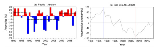
Figure 3.
(a) The time series of the Pacific blocking frequency anomaly in the key area (unit: %). Anomalies are computed by removing long–term mean of key–area Pacific blocking frequency during 40 winters. The dashed lines indicate the mean frequency anomaly during each period. (b) The accumulated anomaly of (a). The |z| in the top is the result of the nonparametric statistics of (b) and the Z denotes the 0.05 significance level in the nonparametric test. The two vertical lines mark the two turning years (i.e., 1988 and 2008).
The PBF in January during the period of 1980–1988, 1989–2008, and 2009–2019 is 79%, 63%, and 79%, respectively. The spatial distribution of the PBF in three periods are displayed in Figure 4. It is seen that the maximum value in the Pacific is less in the second period than that in both the first and the third periods. The maximum value in the three periods is 68%, 48%, 72%, respectively. It is noted that the 68%–covered area is larger in the third period than that in the first period. Figure 4d illustrates the spatial distribution of the PBF difference between the first two periods. It shows that the mid–high–latitude area, especially the region north 55°N, is dominated by a significantly negative anomaly, with the minimum anomaly reaching to −20%. Thus, the Pacific blocking during 1980–1988 is more active than that in the period of 1989–2008. The spatial distribution of the PBF difference between the third period and the second period is displayed in Figure 4e. A significantly positive frequency anomaly is located at the Northeast Asian continent. The maximum frequency anomaly reaches +24%. Besides, similar patterns and numbers are represented based on the 20CRV3 reanalysis dataset (not shown).
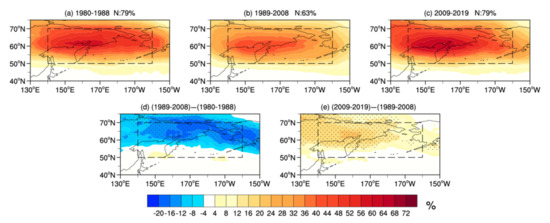
Figure 4.
(a) Horizontal distribution of Pacific blocking frequency (unit: %) in January during 1980–1988; (b) As in (a), but for 1989–2008; (c) as in (a), but for 2009–2019; (d) Difference between (b) and (a); (e) as in (d), but for the difference between (c) and (b). Dotted area indicates the difference exceeding 0.01 significance level. The boxes indicate boundaries of the key area (140° E–160° W, 50°–70° N). The N in the top is the ratio of the total blocking days to the total days in the corresponding month.
Figure 5a,b show the difference of Z500 between the periods in order to address the different circulation between the different periods. The detrended Z500 and T2m are applied in order to remove the influence of global warming. Figure 5a presents the Z500 difference between the second period and the first period (former minus latter). There is a negative Z500 anomaly over the high–latitude area and a positive one over the mid–latitude Pacific. This dipole pattern enhances the gradient of the geopotential height, leading to an anomalous westerly circulation. This is unfavorable to the blocking occurrence. Thus, the PBF is less in the period of 1989–2008 shown in Figure 4d. Figure 5b presents the Z500 difference between the third period and second period. It can be found that the pattern of the statistically significant Z500 anomaly is opposite to that in Figure 5a. This pattern can weaken the Z500 gradient around the Okhotsk Sea, resulting in an easterly anomaly. Accordingly, a greater PBF in the period of 2009–2019 (Figure 4e) is caused.
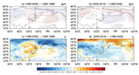
Figure 5.
(a) The difference of the detrended Z500 (unit: gpm) between 1989–2008 and 1980–1988; (b) As in (a), but for the difference between 2009–2019 and 1989–2008. Solid contours are positive values; dashed contours are negative values (interval: 20 gpm; the zero contours omitted). (c) and (d) As in (a) and (b), respectively, but for T2m (unit: K). Yellow shadings are positive T2m anomaly; blue shadings are negative ones. The boxes indicate boundaries of the key area (140°E–160°W, 50°–70°N). Dotted area indicates the anomaly exceeding 0.01 significance level.
Figure 5c,d present the horizontal distribution of the detrended T2m difference between these periods to investigate the relationship of the PBF anomaly to the air temperature. Figure 5c displays the difference between the second and the first periods. As shown, a negative T2m anomaly appears over the high–latitude area and the eastern Pacific area (150°–120° W, 20°–40° N). The high–latitude area is located at the southwest of the negative Z500 anomaly (Figure 5a). It leads to a domination of a northwesterly anomaly and an invasion of the cold air in situ. On the other hand, this eastern Pacific area is located at the southeast of the positive Z500 anomaly (Figure 5a), leading to a northeasterly anomaly and the negative T2m anomaly. A positive T2m anomaly appears over the mid–latitude Pacific area and the Asian area (90°–150° E, 30°–75° N). These areas are dominated by the positive Z500 anomaly (Figure 5a). Figure 5d shows the detrended T2m anomaly between the third period and second period. It is seen that a large range of positive T2m anomaly appears over the high–latitude area, north of the 65°N, and over the eastern Pacific area (150°–120° W, 10°–60° N). These regions are dominated by the positive Z500 anomaly (Figure 5b). A negative T2m anomaly appears over the mid–latitude Asia area (60°–140° E, 40°–60° N) and the western Pacific area (140°–170° E, 20°–50° N). The areas are located at the southeast of positive Z500 anomaly and the west of negative Z500 anomaly (Figure 5b), leading to the northeasterly and northerly anomaly. Figure 5d,e are rerun by 925 hPa air temperature in order to examine the results of T2m anomaly. Similar patterns are obtained, but the numbers are smaller than those that are presented in Figure 5d,e (not shown).
The correlation between the variables (Z500, U200, T2m) and the key–area PBF confirms the results that were obtained from Figure 5. The spatial distribution of the correlation coefficient between the time series of the key–area PBF anomaly shown in Figure 3a and the spatial Z500 field is shown in Figure 6a. Positive coefficient appears at high latitude and negative one appears at mid–latitudes. The methodology [15] is symmetrical in the search that it seeks to identify the poleward blocking anticyclone and the equatorward cutoff cyclone. Therefore, a more active blocking over the Pacific sector corresponds to a positive Z500 anomaly at high–latitude regions and a negative Z500 anomaly at mid–latitude regions, which is consistent with Figure 5a,b. Figure 6b shows the spatial distribution of the coefficient between the key–area PBF time series and the U200 field. As shown, a large range of negative coefficient appears to north of 50°N and a positive coefficient appears over the subtropical region of 15°–30° N. An easterly anomaly to the north of 50° N corresponds to the positive Z500 at high latitude and the negative Z500 anomaly at mid–latitude, following well the geostrophic relationship. In addition, a more active blocking corresponds to an easterly anomaly following the methodology [15]. The positive coefficient in the subtropical region indicates that the increased subtropical jet can impact the Pacific blocking activities [8,9].
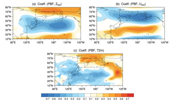
Figure 6.
(a) Horizontal distribution of the correlation coefficient between the time series of the key–area Pacific blocking frequency (PBF) anomaly and Z500 field; (b) as in (a), but for the correlation between the time series and U200 field; (c) as in (a), but for the correlation between the time series and T2m field. Yellow shadings are positive correlation coefficients, and blue shadings are negative ones. The boxes indicate boundaries of the key area (140° E–160° W, 50°–70° N). Dotted area indicates the correlation coefficient exceeding 0.05 significance level.
Figure 6c shows the spatial distribution of the correlation coefficient between the key–area PBF time series and the T2m field. Because a significantly positive coefficient appears at the northeast of Asia and the eastern Pacific, the T2m increases over these regions when the Pacific blocking is more active. This is consistent with the pattern of T2m anomaly at high–latitude region in Figure 5c,d. A significantly negative coefficient area appears over the northeastern Asia and the mid–western Pacific between 15° N and 50° N, which coincides with the positive/negative T2m anomaly over the Eastern Asia and Western Pacific in Figure 5c,d.
4. Conclusions
Using a 2D blocking index, the space–time evolution of the Pacific blocking frequency (PBF) is mainly investigated. It is found that the maximum PBF appears in January. The winter–mean result and the individual winter–month result, the maximum PBF always occurs within the area of 140° E–160° W, 50°–70° N. This area is selected as a key area. Most importantly, the mean frequency anomaly in the key area shows a multi–year change in January, i.e., the Pacific blocking is more active during the first period (1980–1988) and the third period (2009–2019) than the second period (1989–2008).
It is conceded here that the period of study is not long enough to have a clear view of the causes of multidecadal blocking variability at the moment. The Pacific Decadal Oscillation (PDO) or the Atlantic Multidecadal Oscillation (AMO) plays a significant role in the decadal to multidecadal variability of the Northern Hemisphere blocking frequency [17,18]. However, the short observational period (40 years) relative to the time scales of AMO or PDO is difficult to find statistically significant relationships between the weather systems and decadal oceanic modes of variability [16]. On the other hand, the literature [28] indicates that the sea ice cover (SIC) is closely related to blocking frequency. The composite SIC anomaly in January during three periods conclude that the sea ice cover area in the Bering Sea is lower (higher) in the higher (lower) blocking frequency period. Therefore, the underlying mechanism of blocking frequency variability should be further studied by the variability of the local SIC or the local SST.
The local SIC anomaly or SST anomaly will cause a circulation anomaly. The different circulation leads to the PBF anomaly variation among the three periods. The Z500 anomaly between the second period and the first period indicates that the positive anomaly appears over the mid–latitude Pacific and the negative one appears over the high–latitude area. This dipole pattern leads to an anomalous westerly circulation which weakens the blocking activities. The pattern of the statistically significant Z500 anomaly between the third and the second periods is opposite to that between the second and the first periods. Thus, the Z500 anomaly leads to an anomalous easterly strengthens blocking activities. The circulation in the three periods is closely related to the T2m anomaly. The difference of Z500 between the second period and the first period leads to a positive T2m anomaly over the mid–latitude Pacific and the Asian area and leads to a negative T2m anomaly over the high–latitude area and the eastern Pacific area. The difference of Z500 between the third period and the second period leads to the positive T2m anomaly over the 65°–80° N latitudinal band and the eastern Pacific and leads to the negative ones over the mid–latitude Asia and western Pacific.
The analysis of the correlation coefficient between the variables (Z500, U200, T2m) and the key–area PBF confirms the above results. The spatial distribution of the correlation coefficient between the key–area PBF time series and the spatial Z500 field shows that the positive coefficient appears at high latitude and the negative coefficient appears at mid–latitudes. The spatial distribution of the correlation coefficient between the key–area PBF time series and the spatial U200 field shows that a positive coefficient appears over the subtropical region and a large range of negative coefficient appears to north of 50° N. Thus, the easterly anomaly appears to the north of 50° N and the westerly anomaly appears over the subtropical region when the Pacific blocking is more active. In addition, the spatial distribution of the correlation coefficient between the key–area PBF time series and the spatial T2m field shows that a significantly positive coefficient appears at the northeast of Asia and the eastern Pacific and a significantly negative coefficient appears over northeastern Asia and the mid–western Pacific between 15° N and 50° N. This suggests the results of Figure 5c,d.
Author Contributions
Conceptualization, M.G. and S.Y.; methodology, M.G. and S.Y.; software, M.G. and S.Y.; validation, M.G., S.Y. and T.L.; formal analysis, M.G. and S.Y.; investigation, M.G. and S.Y.; resources, S.Y. and T.L.; data curation, M.G.; writing—original draft preparation, M.G.; writing—review and editing, S.Y. and T.L.; visualization, M.G. and S.Y.; supervision, S.Y.; project administration, S.Y.; funding acquisition, S.Y. All authors have read and agreed to the published version of the manuscript.
Funding
This research was funded by the National Key R&D Program of China, grant number 2018YFC1505905 and 2018YFC1505803, the National Natural Science Foundation of China, grant number 41975048, the Natural Science Foundation of Jiangsu Higher Education Institutions of China, grant number 18KJB170015, and the Startup Foundation for Introducing Talent of NUIST, grant number 2018R027.
Acknowledgments
The authors would like to thank the European Centre for Medium–Range Weather Forecasts for the data and information provided.
Conflicts of Interest
The authors declare no conflict of interest.
References
- Rex, D.F. Blocking action in the middle troposphere and its effect upon regional climate. I: An aerological study of blocking action. Tellus 1950, 2, 196–211. [Google Scholar] [CrossRef]
- Masato, G.; Hoskins, B.J.; Woollings, T.J. Wave–breaking characteristics of midlatitude blocking. Q. J. R. Meteorol. Soc. 2012, 138, 1285–1296. [Google Scholar] [CrossRef]
- Buehler, T.; Raible, C.C.; Stocker, T.F. The relationship of winter season North Atlantic blocking frequencies to extreme cold or dry spells in the ERA–40. Tellus 2016, 63, 174–187. [Google Scholar] [CrossRef]
- Pook, M.J.; Risbey, J.S.; McIntosh, P.C.; Ummenhofer, C.C.; Marshall, A.G.; Meyers, G.A. The seasonal cycle of blocking and associated physical mechanisms in the Australian region and relationship with rainfall. Mon. Weather Rev. 2013, 141, 4534–4553. [Google Scholar] [CrossRef]
- Li, C.Y.; Gu, W. An analyzing study of the anomalous activity of blocking high over the Ural Mountains in January 2008. Chin. J. Atmos. Sci. 2010, 34, 865–874. [Google Scholar] [CrossRef]
- Dole, R.; Hoerling, M.; Perlwitz, J.; Eischeid, J.; Pegion, P.; Zhang, T.; Quan, X.-W.; Xu, T.; Murray, D. Was there a basis for anticipating the 2010 Russian heat wave? Geophys. Res. Lett. 2011, 38, 6. [Google Scholar] [CrossRef]
- Masato, G.; Hoskins, B.J.; Woollings, T. Wave–breaking characteristics of Northern Hemisphere winter blocking: A two–dimensional approach. J. Clim. 2013, 26, 4535–4549. [Google Scholar] [CrossRef]
- Henderson, S.A.; Maloney, E.D.; Barnes, E.A. The influence of the Madden–Julian oscillation on Northern Hemisphere winter blocking. J. Clim. 2016, 29, 4597–4616. [Google Scholar] [CrossRef]
- Henderson, S.A.; Maloney, E.D. The impact of the Madden–Julian oscillation on high–latitude winter blocking during El Niño–Southern Oscillation events. J. Clim. 2018, 31, 5293–5318. [Google Scholar] [CrossRef]
- Tibaldi, S.; Molten, F. On the operational predictability of blocking. Tellus 1990, 42, 343–365. [Google Scholar] [CrossRef]
- Scherrer, S.C.; Croci–Maspoli, M.; Schwierz, C.; Appenzeller, C. Two–dimensional indices of atmospheric blocking and their statistical relationship with winter climate patterns in the Euro–Atlantic region. Int. J. Climatol. 2006, 26, 233–249. [Google Scholar] [CrossRef]
- Davini, P.; Cagnazzo, C.; Gualdi, S.; Navarra, A. Bidimensional diagnostics, variability, and trends of Northern Hemisphere blocking. J. Clim. 2012, 25, 6496–6509. [Google Scholar] [CrossRef]
- Berrisford, P.; Hoskins, B.J.; Tyrlis, E. Blocking and Rossby wave breaking on the dynamical tropopause in the Southern Hemisphere. J. Atmos. Sci. 2007, 64, 2881–2898. [Google Scholar] [CrossRef]
- Pelly, J.L.; Hoskins, B.J. A new perspective on blocking. J. Atmos. Sci. 2003, 60, 743–755. [Google Scholar] [CrossRef]
- Masato, G.; Hoskins, B.J.; Woollings, T. Winter and summer Northern Hemisphere blocking in CMIP5 models. J. Clim. 2013, 26, 7044–7059. [Google Scholar] [CrossRef]
- Rohrer, M.; Brönnimann, S.; Martius, O.; Raible, C.C.; Wild, M. Decadal variations of blocking and storm tracks in centennial reanalyses. Tellus 2019, 71, 1. [Google Scholar] [CrossRef]
- Lupo, A.; Jensen, A.; Mokhov, I.; Timazhev, A.; Eichler, T.; Efe, B. Changes in global blocking character in recent decades. Atmosphere 2019, 10, 92. [Google Scholar] [CrossRef]
- Joyce, T.M.; Ummenhofer, C.C.; Seo, H.; Kwon, Y. –O. Impact of multidecadal variability in Atlantic SST on winter atmospheric blocking. J. Clim. 2020, 33, 867–892. [Google Scholar] [CrossRef]
- Hwang, J.; Martineau, P.; Son, S.W.; Miyasaka, T.; Nakamura, H.J.J.o.t.A.S. The role of transient eddies in North Pacific blocking formation and its seasonality. J. Atmos. Sci. 2020, 77, 2453–2470. [Google Scholar] [CrossRef]
- Davini, P.; D’Andrea, F. Northern hemisphere atmospheric blocking representation in global climate models: Twenty years of improvements? J. Clim. 2016, 29, 8823–8840. [Google Scholar] [CrossRef]
- Hinton, T.J.; Hoskins, B.J.; Martin, G.M. The influence of tropical sea surface temperatures and precipitation on north Pacific atmospheric blocking. Clim. Dyn. 2009, 33, 549–563. [Google Scholar] [CrossRef]
- Woollings, T.; Barriopedro, D.; Methven, J.; Son, S.W.; Martius, O.; Harvey, B.; Sillmann, J.; Lupo, A.R.; Seneviratne, S. Blocking and its response to climate change. Curr. Clim. Chang. Rep. 2018, 4, 287–300. [Google Scholar] [CrossRef]
- Yang, S.Y.; Tim, L. The role of intraseasonal variability at mid–high latitudes in regulating Pacific blockings during boreal winter. Int. J. Climatol. 2017, 37, 1248–1256. [Google Scholar] [CrossRef]
- Woollings, T.; Hoskins, B.; Blackburn, M.; Berrisford, P. A new Rossby wave–breaking interpretation of the North Atlantic Oscillation. J. Atmos. Sci. 2008, 65, 609–626. [Google Scholar] [CrossRef]
- Dee, D.P.; Uppala, S.M.; Simmons, A.J.; Berrisford, P.; Poli, P.; Kobayashi, S.; Andrae, U.; Balmaseda, M.A.; Balsamo, G.; Bauer, P.; et al. The ERA–interim reanalysis: Configuration and performance of the data assimilation system. Q. J. R. Meteorol. Soc. 2011, 137, 553–597. [Google Scholar] [CrossRef]
- Barriopedro, D.; Garcí-Herrera, R.; Trigo, R.M. Application of blocking diagnosis methods to General Circulation Models. Part I: A novel detection scheme. Clim. Dyn. 2010, 35, 1373–1391. [Google Scholar] [CrossRef]
- Slivinski, L.C.; Compo, G.P.; Whitaker, J.S.; Sardeshmukh, P.D.; Giese, B.S.; McColl, C.; Allan, R.; Yin, X.; Vose, R.; Titchner, H.; et al. Towards a more reliable historical reanalysis: Improvements for version 3 of the Twentieth Century Reanalysis system. Q. J. R. Meteorol. Soc. 2019, 145, 2876–2908. [Google Scholar] [CrossRef]
- Yao, Y.; Luo, D.; Zhong, L. Effects of northern hemisphere atmospheric blocking on arctic sea ice decline in winter at weekly time scales. Atmosphere 2018, 9, 331. [Google Scholar] [CrossRef]
© 2020 by the authors. Licensee MDPI, Basel, Switzerland. This article is an open access article distributed under the terms and conditions of the Creative Commons Attribution (CC BY) license (http://creativecommons.org/licenses/by/4.0/).