Article

Evaluation of the Antarctic Circumpolar Wave Simulated by CMIP5 and CMIP6 Models

1
Key Laboratory of Meteorological Disaster, Ministry of Education/Joint International Research Laboratory of Climate and Environment Change/Collaborative Innovation Center on Forecast and Evaluation of Meteorological Disasters, Nanjing University of Information Science and Technology, Nanjing 210044, China
2
Key Laboratory of Regional Climate-Environment Research for Temperate East Asia, Institute of Atmospheric Physics, Chinese Academy of Science, Beijing 100029, China
*
Author to whom correspondence should be addressed.
Atmosphere 2020, 11(9), 931; https://doi.org/10.3390/atmos11090931
Submission received: 13 July 2020 / Revised: 27 August 2020 / Accepted: 28 August 2020 / Published: 30 August 2020
(This article belongs to the Section Climatology)

Abstract

:
As a coupled large-scale oceanic and atmospheric pattern in the Southern Ocean, the Antarctic circumpolar wave (ACW) has substantial impacts on the global climate. In this study, using the European Centre for Medium-Range Weather Forecasts ERA5 dataset and historical experiment outputs from 24 models of the Coupled Model Intercomparison Project Phase 5 and Phase 6 (CMIP5/CMIP6) spanning the 1980s and 1990s, the simulation capability of models for sea-level pressure (SLP) and sea surface temperature (SST) variability of the ACW is evaluated. It is shown that most models can capture well the 50-month period of the ACW. However, many simulations show a weak amplitude, but with various phase differences. Selected models can simulate SLP better than SST, and CMIP6 models generally perform better than the CMIP5 models. The best model for SLP simulation is the CanESM5 model from CMIP6, whereas the best model for SST simulation is the ACCESS1.3 model from CMIP5. It seems that the SST simulation benefits from the inclusion of both a carbon cycle process and a chemistry module, while the SLP simulation benefits from only the chemistry module. When both SLP and SST are taken into consideration, the CanESM5 model performs the best among all the selected models.

1. Introduction

The Antarctic circumpolar wave (ACW) is a large-scale air-sea interactive phenomenon in the Southern Hemisphere, first named by White and Peterson in 1996 [1]. It manifests as an eastward-propagating signal around the Antarctic in sea-level pressure (SLP) [1,2,3,4], sea surface temperature (SST) [1,2,3,4,5,6,7], sea-ice extent/sea-ice concentration (SIE/SIC) [1,8,9], sea surface height (SSH) [5,10], meridional wind speed (MWS) [1,6,11,12], wind stress [5,10], surface air temperature (SAT) [9,11,13] and salinity [3,11,13], with a mean speed of 6–8 cm s−1 and a period of 4–5 years. As a major component of the Southern Ocean (SO), the ACW plays an important role in the Southern Hemisphere and global climate change and has drawn wide interest around the world [14]. In the past two decades, many researchers have investigated its origin, maintenance mechanism, development, variation and impact on both regional and global climate via statistical diagnostics and numerical modeling. Therefore, various hypotheses and theoretical models have been developed. Qiu and Jin [15] used a coupled model to show that the instability of the coupled ocean-atmosphere interaction is the main source of the ACW. Nevertheless, the ACW in SST anomalies is principally modulated by the El Niño-Southern Oscillation (ENSO) teleconnections [11,16]. It has been suggested that ENSO is responsible for the generation of the ACW [17]. Moreover, it has been found that the ACW can explain the ENSO variability during the last half of the twentieth century and that it will continually influence ENSO under global warming [18]. Bonekamp et al. [3] found that a one-way atmosphere-ocean coupling is sufficient to generate the ACW signature in the SAT, while Venegas [19], along with White and Chen [20], considered that a combination of two different mechanisms that include coupled air-sea interactions is needed. As a climate indicator, the ACW sheds lights on the prediction of regional anomalies several seasons ahead. White and Cherry found that the SST anomaly in the ACW is closely related to the autumn-winter precipitation in New Zealand, and it surpasses ENSO as an indicator [6]. White found that the ACW has a great impact on Australian interannual precipitation and that it can explain most variations in specific regions [21]. According to Prabhu et al., the ACW not only affects the high latitudes of the Southern Hemisphere but also influences the Subtropical Front via the tropospheric response [22] and modulates the extremes of the Indian summer monsoon rainfall via SST and the upper tropospheric meridional transport of heat over the southeast Pacific [23]. Recently, some Chinese researchers have also investigated its evolution dynamics and climate influence. Xiao et al. found a regular phase difference between the SLP and SST signals in the South Indian Ocean from 1980 to 1996 [24]. Bian and Lin found that the ACW experienced a shift from wavenumber 3 to wavenumber 2 in 1972 [25]. They further pointed out that ACW has featured a wavenumber 2 pattern and eastward propagation since the 1980s [26]. Xie et al. found that the ACW has a close link to the summer precipitation anomalies in China [18]. However, because of the poor observation density and lack of long-term observations, it is difficult to study the ACW over a long period, let alone comprehensively understand the dynamics and its impacts on the climate.
However, studies using a climate-model-simulated ACW have achieved much progress. Researchers have used coupled air-sea models with a sea-ice module [27,28,29,30] and global model coupling atmospheric, oceanic, sea ice and biospheric components [31] to investigate the evolution features and driving mechanisms of the ACW. In these studies, the problems of unfixed ACW fluctuation periods and various fluctuation features in different models have been highlighted. For example, Motoi used the MRI-GCM-1 model and obtained a period of 10–15 years [27], while Christoph et al. simulated the ACW using the MPI-CGCM model and found a period of 12–16 years. It was also found that the ACW variability is mainly dominated by the variation of wavenumbers 2–4 on the century timescale [30,31]. As mentioned above, the lack of reference data and the defects of numerical models contribute to the large uncertainties in these research results, which needs further confirming by using the latest climate models.
Conducted by The Working Group on Coupled Modelling (WGCM), the completed CMIP5 included more than 40 models and promoted a standard set of model simulations in order to: (1) Evaluate how realistic the models are in simulating the recent past. (2) Provide projections of future climate change on two time scales, near term (out to about 2035) and long term (out to 2100 and beyond). (3) Understand some of the factors responsible for differences in model projections. Started in 2016, the ongoing CMIP6 with over 70 models, which generally have a finer resolution and improved dynamical processes to their family predecessors in CMIP5, continues the pattern of evolution and adaptation characteristic of CMIP5. These multimodel results are currently widely used in many areas of climate research [32,33]. They are a useful research tool to deeply understand the sources and evolution of climate change and the response in future scenarios, playing a vital role in climate change assessments and international negotiations. Yet it is still uncertain how well these models can simulate the ACW and whether they can be used in ACW research. To partly answer these questions, this study focuses on evaluating the ability of multiple CMIP5 and CMIP6 models to simulate the ACW, with the aim of increasing the knowledge about the ACW.

2. Data and Methods

2.1. Gridded Datasets

Owing to the scarcity of observations in the SO, reanalysis data is used here to define the ACW. According to Marshall [34], the ERA reanalysis dataset from the European Centre for Medium-Range Weather Forecasts (ECMWF) can well depict high-latitude circulations in the Southern Hemisphere. Therefore, the monthly SLP and SST product from the ERA5 dataset [35] was used as the reference data for comparison with numerical model results. The spatial resolution was interpolated to 1° × 1° and the temporal range was from January 1979 to December 1997. The SLP and SST output from 12 CMIP5 and 12 CMIP6 models’ historical experiments were also collected to evaluate their ability to simulate the ACW (Table 1). The first six of the CMIP5 models were physical climate system models and the last six models were Earth system models with a carbon cycle process [36]. The CMIP6 models were the latest version of the corresponding CMIP5 models. The CNRM-CM6-1 model includes an atmospheric chemistry module, the IPSL-CM6A-LR model includes an oceanic chemistry module, and the CESM2, GFDL-CM4, CanESM5 and GFDL-ESM4 models include both of these modules. For comparison, all model results were bilinearly interpolated into the same grid as the ERA5 data.

2.2. Taylor Analysis

The Taylor analysis is widely used to evaluate model simulations against reference data. It draws a diagram that can provide a concise statistical summary of how well patterns match each other in terms of their correlations, their root-mean-square differences and the ratios of their variances [37]. Then we can calculate the skill score S of each model as:
S = 4 ( 1 + R ) 4 ( σ + 1 σ ) 2 ( 1 + R 0 ) 4
where R is the pattern correlation between the reference and simulation, σ is the simulated standard deviation divided by that of the reference (also normalized standardized deviation) and R 0 represents the maximum of probable correlation coefficient (here set as 1). S ranges from 0 to 1. The closer S is to 1, the better simulation skill the model has.

2.3. ACW Extraction

There are several definitions of the ACW, and here we followed in the steps of White and Peterson [1]. First, the monthly anomalies were calculated to remove the seasonal cycle, then a bandpass filter of 3–7 years was used to remove the fast change and long-term signals. To avoid the boundary effect, the data from 4 year before and after the study period were omitted. A small difference is that we used the Butterworth filter with a flat amplitude response function, which is commonly used in ACW studies [16,31,38,39]. The empirical orthogonal function (EOF) was applied to filter monthly anomalies, and the first mode (EOF1) represents the ACW signal [16,25]. Moreover, a spectrum analysis was carried out to obtain a clear period.
In the following section, results from the reference data, the model with the highest skill score, the unweighted average of the CMIP5 and CMIP6 model ensembles and the models in CMIP5 and CMIP6 with the highest correlation with the reference data are shown.

3. Results

3.1. Taylor Analysis of Model Simulations

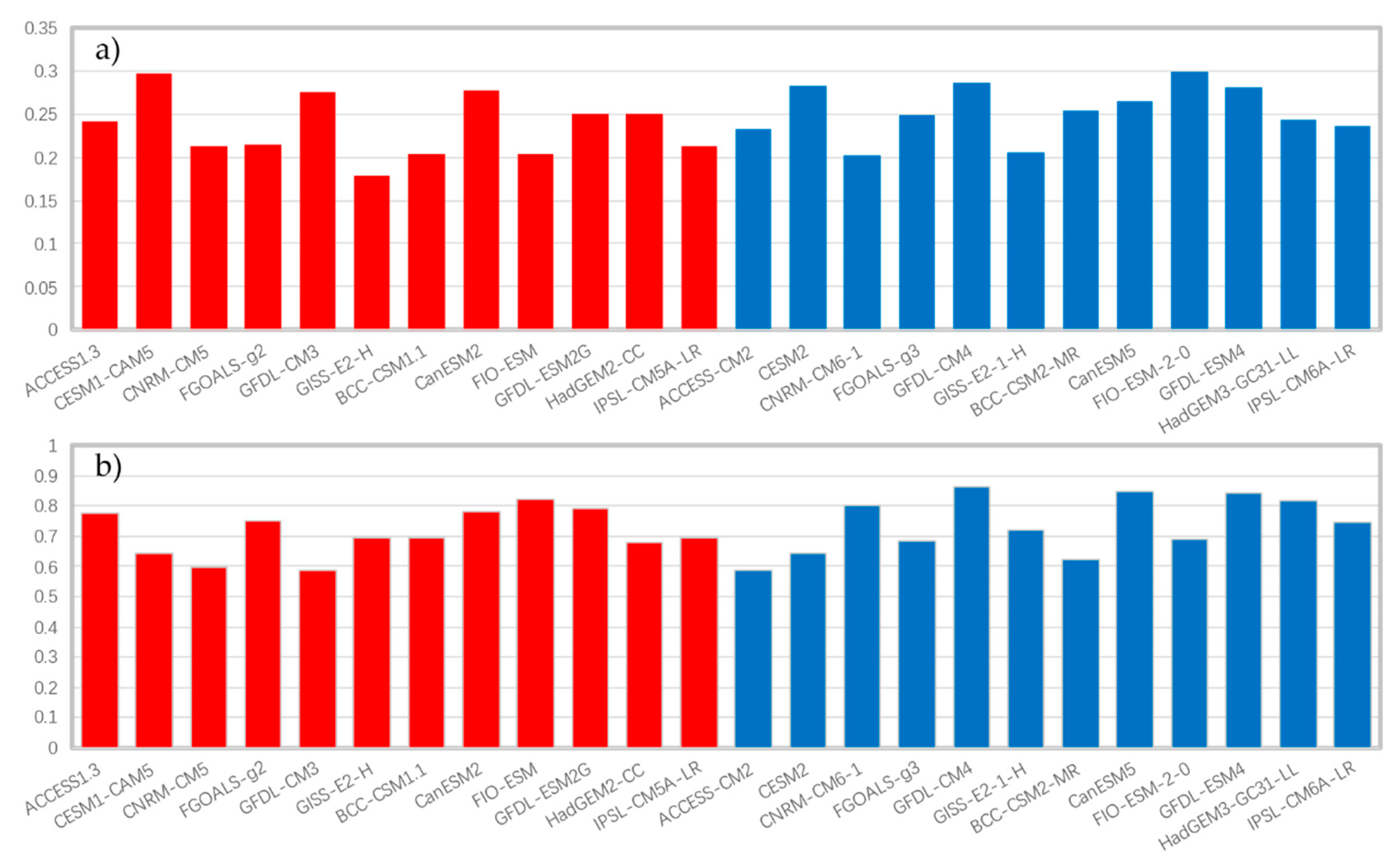
The Taylor analysis was applied to pick up well simulated SLP and SST for further evaluation. Figure 1a shows the results for the SLP. Twelve CMIP5 models had normalized and standardized deviation ranging from 0.9 to 1.1 except for the IPSL-CM5A-LR and BCC-CSM1.1 model. The BCC-CSM1.1 model simulated a weaker-centered SLP variance with a normalized and standardized deviation less than 0.9, while the IPSL-CM5A-LR model simulated a stronger-centered SLP variance with normalized and standardized deviation near 1.2. Correlation coefficients between all the models and reference data were larger than 0.3. The CESM1-CAM5 model had the highest S score while the GISS-E2-H model had the lowest. Earth system models show no obvious advantage over physical climate system models (Figure 2a). For the 12 CMIP6 models, normalized and standardized deviation ranged from 0.92 to 1.12, except for the CESM2 model, which was slightly larger. All CMIP6 models’ correlation coefficients were larger than 0.3. The FIO-ESM-2-0 model had the highest S score while the CNRM-CM6-1 model had the lowest. Models with an atmospheric chemistry module had a higher S score than the other models, with the exception of the CNRM-CM6-1 model (Figure 2a). Compared with the CMIP6 models, CMIP5 models generally had poorer correlation coefficients and larger variances between models. The CMIP6 model ensemble was superior to the CMIP5 model ensemble, but not at all times. The FIO-ESM-2-0 model had the highest S score among all 24 models, and thus was considered the best in simulating the reference SLP.
Same as Figure 1a but for SST, Figure 1b shows that 5 out of the 12 CMIP5 models had normalized and standardized deviations of less than 1, meaning that these model-simulated centered SST variances were weaker than the reference data. All CMIP5 models had correlation coefficients over 0.75, among which the FIO-ESM model had the highest, over 0.9. Moreover, the FIO-ESM model had the highest S score while the GFDL-CM3 model had the lowest, and Earth system models seemed to surpass physical climate system models (Figure 2b). Among the 12 CMIP6 models, the CNRM-CM6-1, GISS-E2-1-H and IPSL-CM6A-LR models simulated stronger-centered SST variances than the reference data. In contrast, those in other models were weaker, with the weakest being the CESM2 model with a normalized and standardized deviation of less than 0.75. Correlation coefficients of four models (GFDL-CM4, CanESM5, GFDL-ESM4 and HadGEM3-GC31-LL) exceeded 0.9, and those of all 12 models were over 0.76. The GFDL-CM4 model had the highest S score while the ACCESS-CM2 model had the lowest. Except for the CESM2 model, all models with a chemistry module performed better than those without (Figure 2b). Besides lower normalized standardized deviations, the CMIP6 model ensemble was generally superior to the CMIP5 model ensemble, except for some particular model versions. The GFDL-CM4 model was selected as the best among all 24 models in simulating the reference SST.
In general, both the CMIP5 and CMIP6 models can better simulate SST than SLP. The CMIP6 model ensemble has little advantage over the CMIP5 model ensemble. A chemistry module seems to improve the performance of both SLP and SST simulations. In contrast, the carbon cycle process brings benefits only to the SST simulation.

3.2. Evaluation of Model-Simulated SLP

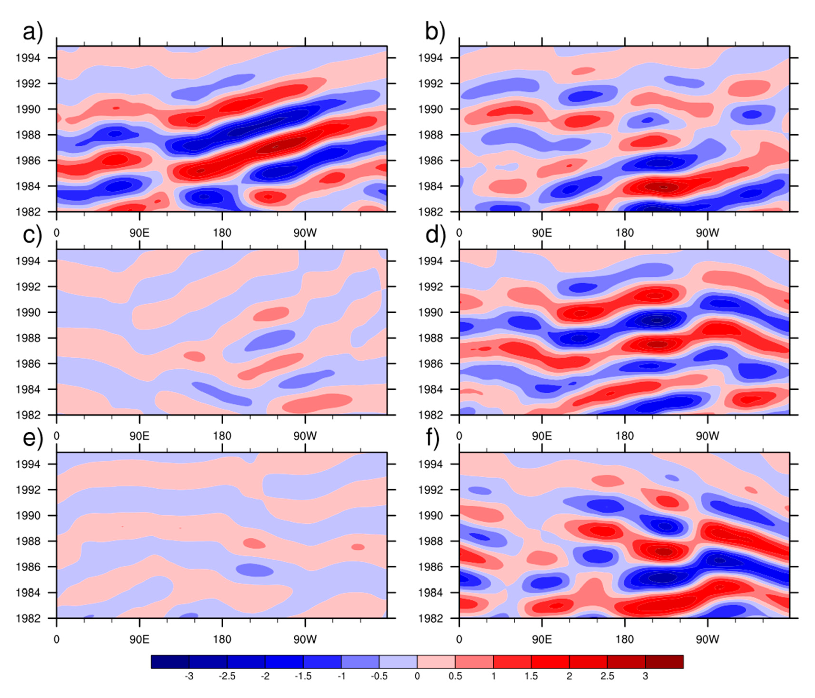
The time-longitude figure shows the evolution of the filtered SLP signal from the reference data (Figure 3a), the best simulation from the FIO-ESM-2-0 model selected via the Taylor analysis (Figure 3b), the unweighted average of both CMIP5 (Figure 3c) and CMIP6 model ensembles (Figure 3e), the CESM1-CAM5 model simulation selected from CMIP5 (Figure 3d) and the CanESM5 model simulation selected from CMIP6 (Figure 3f). There was an obvious annual oscillation at a particular longitude, and a peak to valley pattern appeared in parallel at the same time. This ACW-like pattern shows a dominant eastward propagation, which was most intense and clear in the Pacific sector. The pattern had two wavelengths that encircled the globe with an average period of 6–8 years, which is consistent with previous studies [1,28]. Compared with White and Peterson [1], our result had a 15% (0.5 hPa) weaker amplitude of fluctuation. When the result sensitivities to different data and filters were taken into consideration, it is reasonable to conclude that these reference data could well reproduce the ACW during our study period. The selected CESM1-CAM5, FIO-ESM-2-0 and CanESM5 models basically captured the wave pattern and propagating trend when compared with the reference result. In contrast, the CMIP5 and CMIP6 model ensembles barely show a propagating wave-like pattern. The neutralization of different simulated ACW signals may be responsible for this bad result obtained via the unweighted mean. Among the CMIP5 models, Earth system models show no notable difference from the physical climate models. However, there were several models with poor performance, such as the BCC-CSM1.1 model, which reproduced a random meridional distribution and barely half of the peak value. Although it shows a small eastward-propagating trend, it is among the worst simulations when the vague wave pattern was considered. Moreover, instead of a propagating pattern, the FGOALS-g2 result rather shows a zonally uniform annual oscillation, which greatly differed from the ACW. For CMIP6 models, the CESM2 and HadGEM3-GC31-LL models could not reproduce the wave pattern or propagation trend of the ACW (figure omitted).
It is interesting to notice an abnormal westward propagation between 0 and 90 °W (South Atlantic, including the Drake Passage region) in many models, especially for physical climate models, which cannot be seen in reference data. According to White and Peterson [1], the ACW SST anomalies originate in the western subtropical South Pacific and propagate eastward, which is mainly due to the Antarctic circumpolar current (ACC). The ACC in the Drake Passage region is extremely strong with a velocity of 3–15 cm s−1 that would affect the ACW signal propagation in model simulations [27] and may block the eastward propagation in a specific region [13]. Moreover, the ACW signal tends to be much weaker in the South Atlantic sector [31]. Therefore, there may be large uncertainties for models in simulating the ACC or the mechanisms of how the ACC influences the ACW, making the simulated westward propagation trend rather dubious [40].
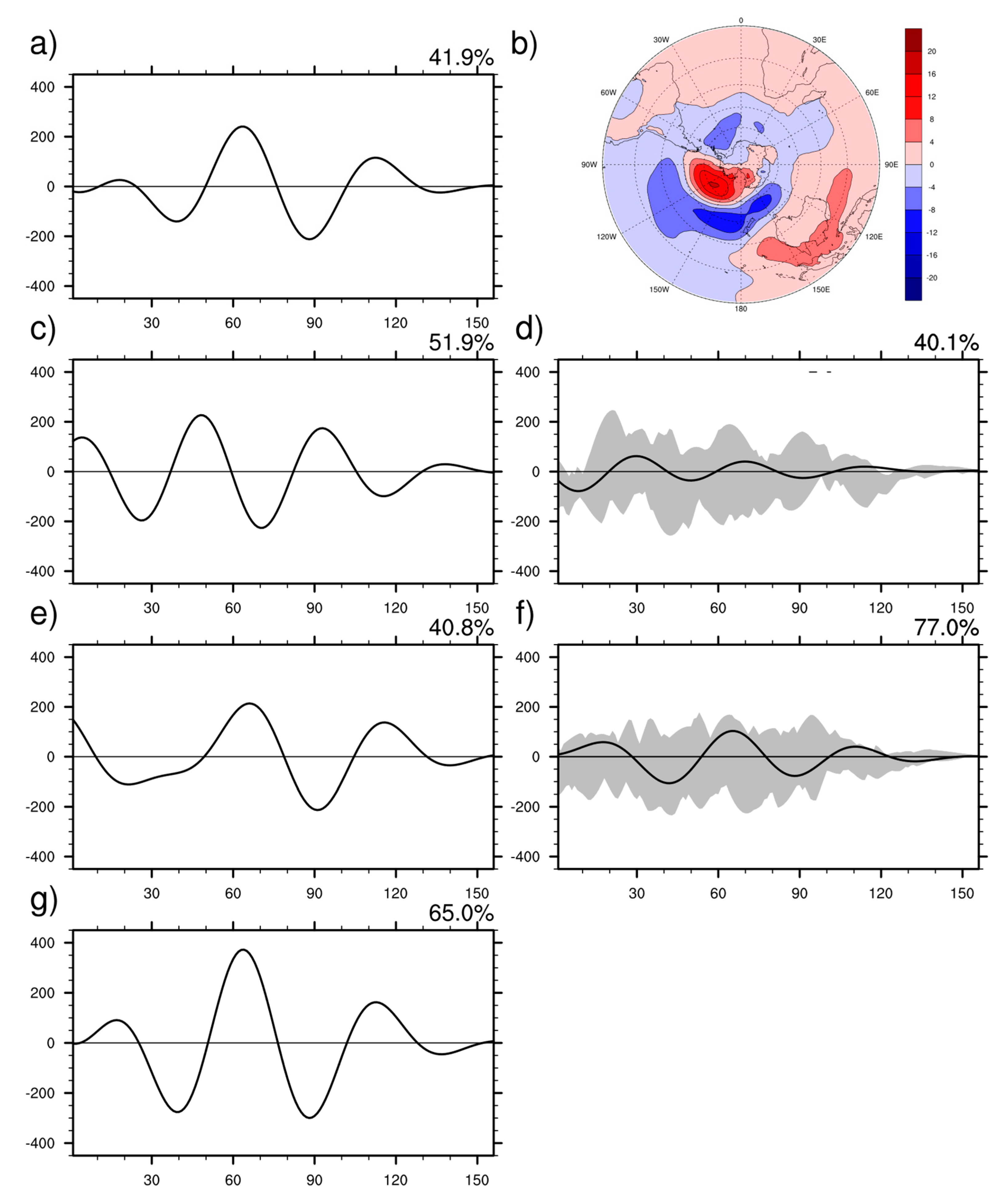
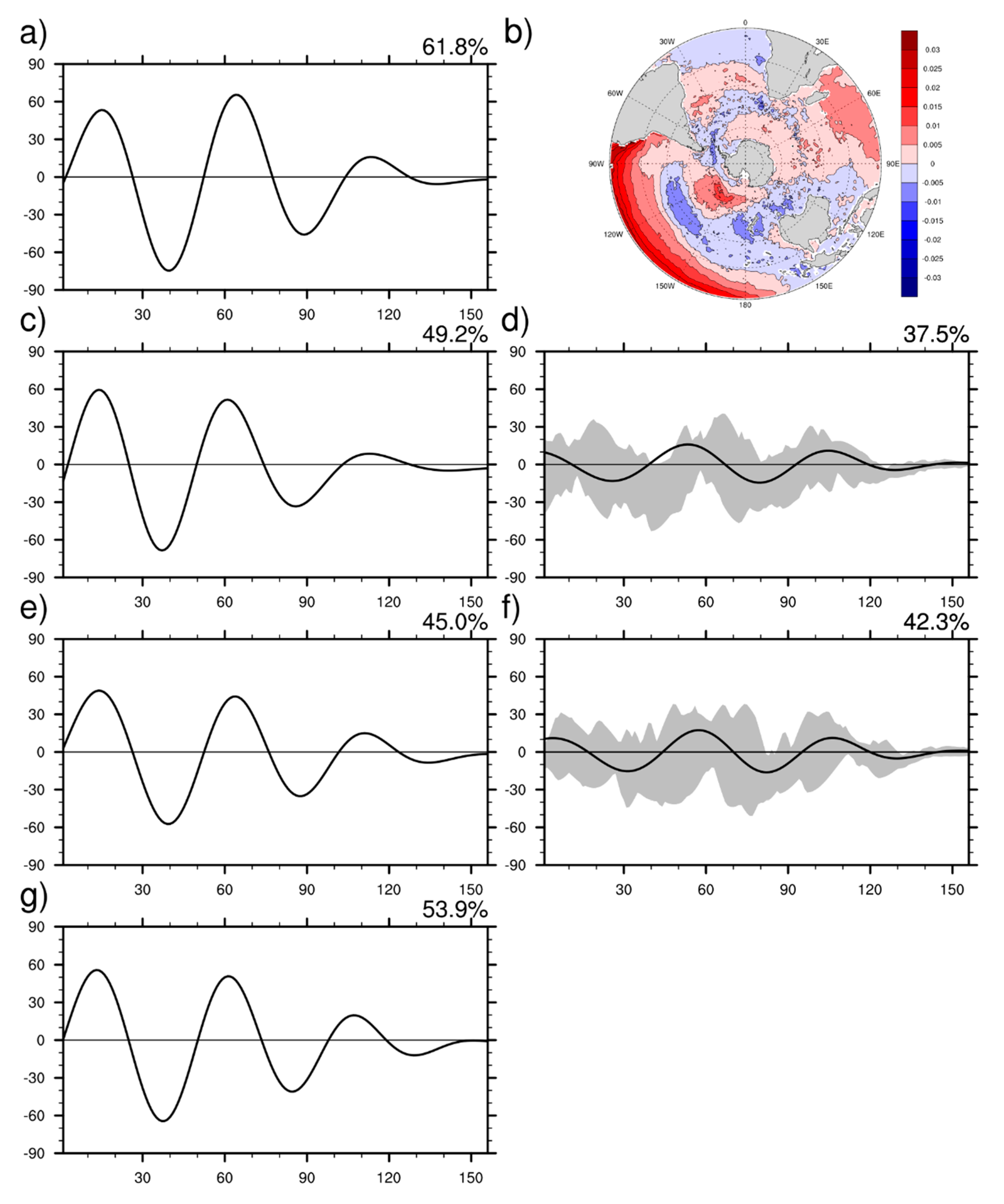
To further investigate the ability of models in simulating the SLP signal, an EOF analysis was applied to the filtered series mentioned above. Figure 4 shows the first EOF mode representing the ACW. As the main mode, the EOF1 of the reference data explained 41.9% of the total variance and took the general form of three complete wavelengths in time series (Figure 4a). This is consistent with the result of Bian and Lin [25], in which the EOF1 explains 33% of the total variance. The CESM1-CAM5 model from CMIP5 explained a little less than the reference data (Figure 4e), while for other models, such as the FIO-ESM model, the explanation rates exceeded 75% (figure omitted). All models had clear fluctuations but varied considerably in wavenumbers and phases (Figure 4d). Furthermore, by calculating the correlation coefficients between the time series of the reference data and model simulations (results omitted), four models—ACCESS1.3, CESM1-CAM5, BCC-CSM1.1 and FIO-ESM—were found to be significantly positively related to the reference data. The CESM1-CAM5 model had the largest correlation coefficient of over 0.85. However, it failed to reproduce the first ACW in the early 1980s. Among the CMIP6 models, CanESM5’s EOF1 explanation rate reached 65% (Figure 4g) and had a positive correlation coefficient of 0.99. Models with an atmospheric chemistry module seem to have a higher positive correlation than those without, although they show no advantage in terms of explaining the total variance. Compared with CMIP5 models, CMIP6 models show no improvement in terms of explained variance but had better performance in fluctuation manifestation.
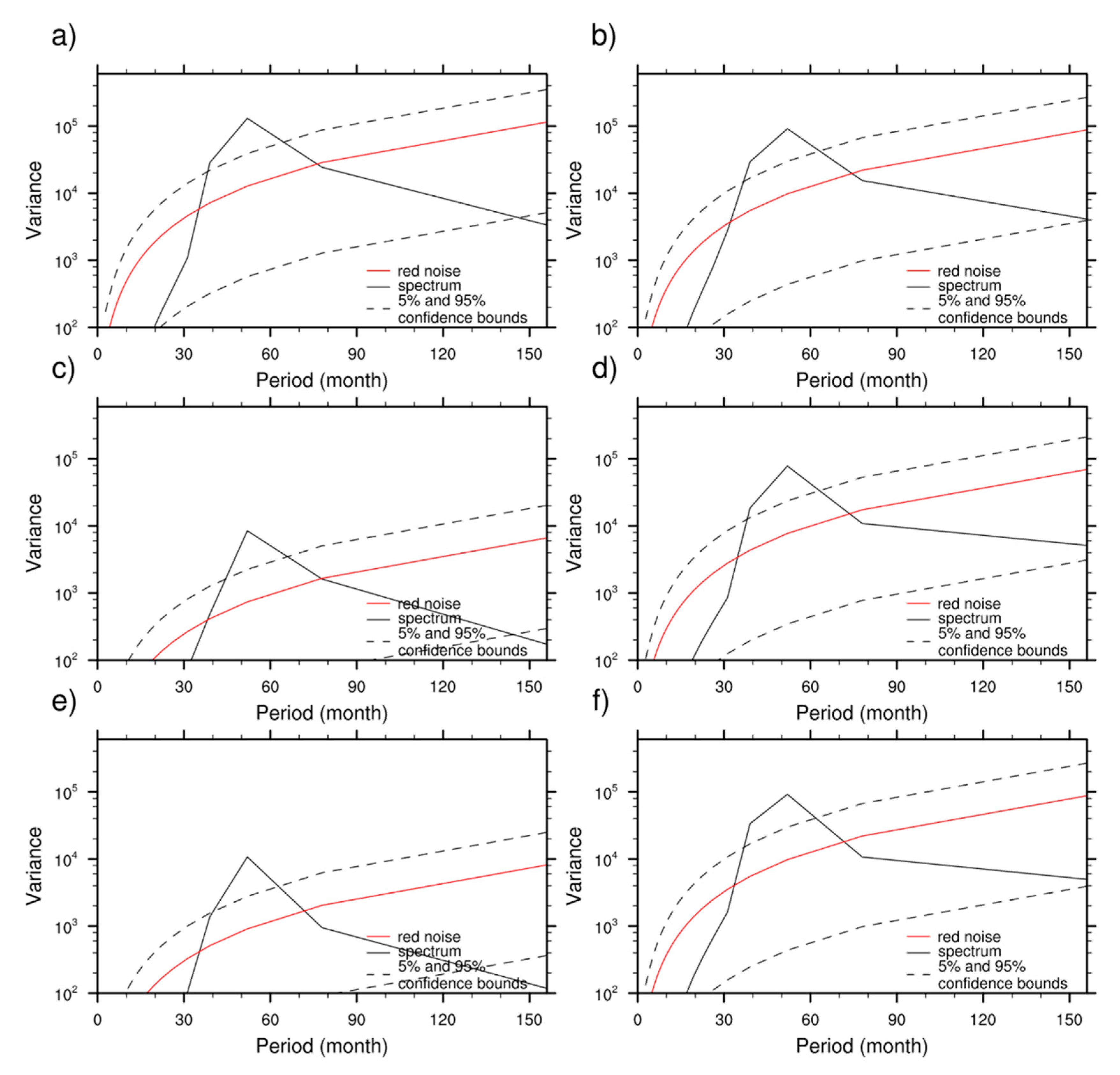
The spectrum analysis of the EOF1 time series was employed to extract the clear period of the ACW (Figure 5). Seven out of 12 CMIP5 models show a nearly 50-month period of the ACW, similar to the reference data (passing the 95% red noise confidence level). Among the other five models, the BCC-CSM1.1, GFDL-ESM2G and IPSL-CM5A-LR models had a major period of 40 months while the CNRM-CM5 and GFDL-CM3 models contained two signals of both 30-month and 50-month periods. Except a 40-month period for the FGOALS-g3 and GFDL-CM4 models, all CMIP6 models show a 50-month period signal as well. Compared with the CMIP5 models, the CMIP6 models reproduce the ACW period better, but the carbon cycle process and chemistry module make no contribution to the better period performance.
Hence, we concluded that three models could simulate the ACW SLP signal well: the FIO-ESM model from CMIP5, and the CanESM5 and GFDL-ESM4 models from CMIP6.

3.3. Evaluation of Model-Simulated SST

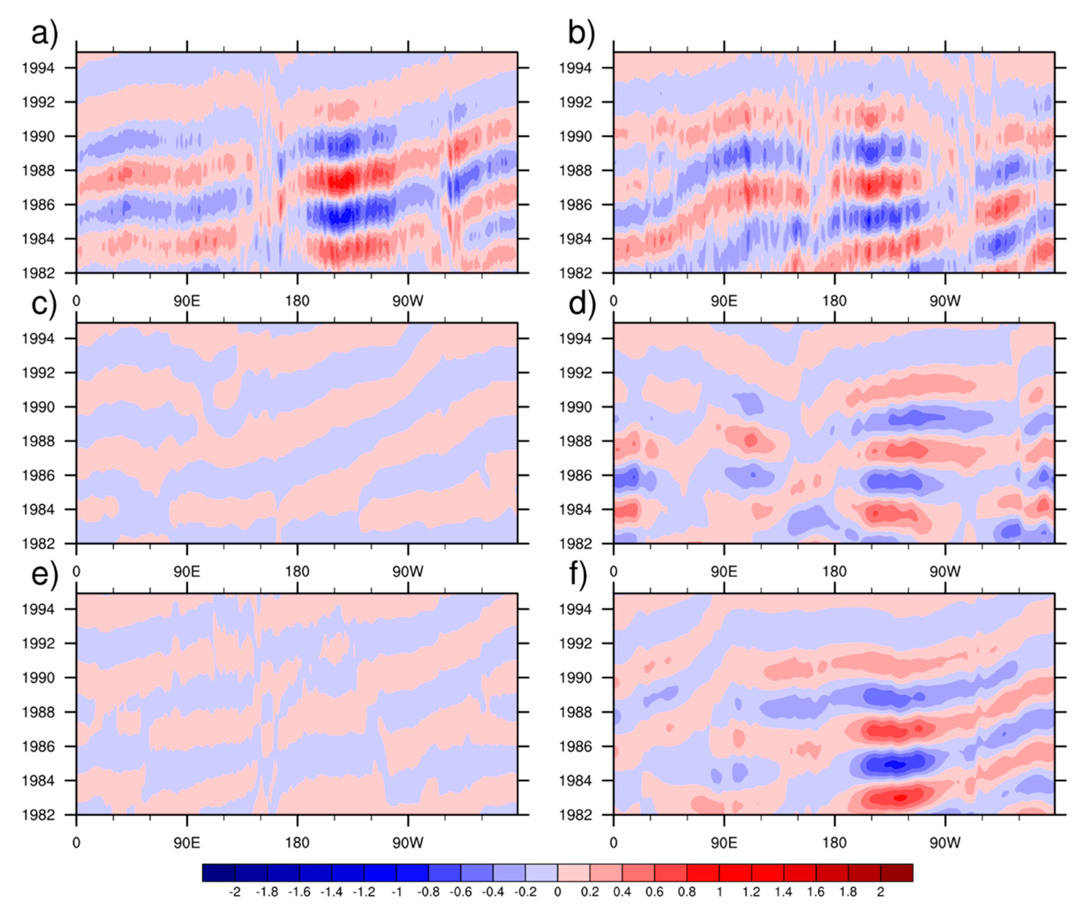
Same as Figure 3, Figure 6 shows the evolution features of the spatiotemporal variation of SST from the reference data (Figure 6a), the best-performing model, GFDL-CM4, selected according to Taylor analysis (Figure 6b), the unweighted average of the CMIP5 model ensemble (Figure 6c) and the CMIP6 model ensemble (Figure 6e), the ACCESS-1.3 model simulation selected form CMIP5 (Figure 6d) and the CESM2 model simulation selected from CMIP6 (Figure 6f). The reference data result was similar to the SLP features, which shows an obvious annual oscillation at a particular longitude and a peak to valley pattern in parallel at the same time. The wave pattern propagated eastward and took about 8 year to encircle the Antarctic. Furthermore, it reconfirmed the findings that the ACW is the strongest in the South Pacific sector in previous studies [11,38,41] and provided confidence regarding the ability of the reference data in capturing real ACW features. Unsatisfactory simulations, such as the BCC-CSM1.1 model, had a small eastward-propagating trend but a fragmentary wave pattern, and the GISS-E2-H model was 50% less than the reference data in amplitude. The ACCESS1.3 model represents the SST signal well in the eastern hemisphere but blurred the propagation trend in the western hemisphere. It took the CESM1-CAM5 model 6 year to encircle the Antarctic, while it took 4 year for the CanESM2 model. In contrast, the CMIP6 models were much improved in representing the wave pattern and propagation trend. The best GFDL-CM4 model result was similar to the reference data with a two-wavelength parallel form and 8 year encircling period. The CESM2 model performed well in the western hemisphere but had a small amplitude in the eastern hemisphere, therefore blurring the ACW. Other models had various problems, such as having a one-third loss in amplitude for the HadGEM2-CC model and a quasi-biennial oscillation instead of the ACW for the BCC-CSM2-MR model (figure omitted).
By applying the EOF analysis to filtered monthly SST anomalies, EOF1 was still taken as the ACW and its time series is shown in Figure 7. The reference data result shows three complete waves and explained over half of the total variance. It exceeded the SLP result, which indicates that there were too many short-time signals in the atmosphere to filter out, while in the ocean, long-time signals were strong and steady, resulting in a high signal-to-noise ratio. Only 1 out of 12 CMIP5 models, namely, the FIO-ESM model, had a larger explanation rate than the reference data, while three, the FGOALS-g3, GISS-E2-1-H and BCC-CSM models, had small explanation rates of less than 40%. The EOF1 time series of the ACCESS1.3, CNRM-CM5, BCC-CSM1.1 and FIO-ESM models were significantly positively related to the reference data result, with the ACCESS1.3 model reaching the highest, over 0.98. However, all CMIP6 models had a lower explanation rate than the reference data, and the HadGEM3-GC31-LL model had the lowest of around 33%. This is consistent with the Taylor analysis result mentioned in Section 3.1, suggesting a weaker SST signal in the CMIP6 model simulations. One more thing to notice is that the three models with a chemistry module, i.e., the CESM2, GFDL-CM4 and CanESM5 models, had significantly positive correlations with the EOF1 time series from the reference data, supporting the above finding that the chemistry module helps to improve SST simulations.
Figure 8 shows the spectrum analysis result of the SST EOF1 time series. The peak of the reference data exactly corresponded to the 50-month period of the ACW and passed over the 95% red noise confidence level. The ACCESS1.3 model also generated a similar spectrum. Among the other CMIP5 models, FGOALS-g2′s main peak failed the significance test, and the significant period of the GISS-E2-H and FIO-ESM models was below 40 months while that of the IPSL-CM5A-LR model exceeded 70 months. However, all CMIP6 models except FIO-ESM-2-0 reproduced the 50-month significant period of the ACW. In general, CMIP6 models could simulate the ACW period more accurately than CMIP5 models, especially those with a chemistry module.
In summary, five models could simulate the SST signal of the ACW well: the ACCESS1.3 and CNRM-CM5 models from CMIP5, and the CESM2, GFDL-CM4 and CanESM5 models from CMIP6.

4. Conclusions

The ACW is a crucial air-sea coupling system in the Southern Hemisphere, and it further influences the global climate. Using White and Peterson’s method of extracting the ACW from SLP and SST fields, we compared the simulated ACWs from historical experiments of the CMIP5 and CMIP6 models with those from the ERA5 data during the most active period of the 1980s and 1990s. The main findings were as follows.
(1)
For SLP simulation, models had low correlations with the reanalysis data. The CMIP6 models show a slightly better performance than the CMIP5 models. Three models, namely, the FIO-ESM model from CMIP5 and the CanESM5 and GFDL-ESM4 models from CMIP6, performed well. Models with an atmospheric chemistry module had better simulations.
(2)
For SST simulation, the CMIP6 models reproduced weaker but more reliable signals than the CMIP5 models. Five models, the ACCESS1.3 and CNRM-CM5 models from CMIP5 and the CESM2, GFDL-CM4 and CanESM5 models from CMIP6, performed well. Models with a carbon cycle process and a chemistry module tended to produce better simulations.
(3)
When both SLP and SST were taken into consideration, most CMIP6 models show an improvement compared with the CMIP5 version. Models simulated SST better than SLP. The best simulation was produced by the CanESM5 model. Most models could capture the 50-month period of SLP and SST signals in the ACW. The main problem remained in generating the correct phase.
It should to be clear that here we evaluated the ACW SLP and SST signals separately without considering their correlation; however, they had stable phase differences. Further research may investigate other variables and introduce the correlations between them. Moreover, the physical mechanism of the model spread remains as further research. Finally, although the EOF method has advantages in presenting the ACW in the form of a standing wave, it cannot reveal the propagation trend [16,42]. More sufficient statistical methods and new appropriate variables representing the ACW should be adopted in future studies to deepen our understanding.

Author Contributions

Z.L. designed the research, processed the meteorological data, and wrote the manuscript. Z.L., T.Z. and W.Z. contributed scientific discussion. Z.L., T.Z. and W.Z. contributed to reviewing the manuscript. All authors have read and agreed to the published version of the manuscript.

Funding

This research was funded by the National Key Research and Development Program of China (2016YFA0600402, 2018YFC1507704), the Strategic Priority Research Program of Chinese Academy of Sciences (XDA20020201) and the National Natural Science Foundation of China (41675094, 41975115, 41475091).

Acknowledgments

Figures were produced using the NCAR Command Language (NCL). The ERA5 reanalysis data were downloaded from (https://cds.climate.copernicus.eu). The CMIP5 model data were downloaded from (https://esgf-node.llnl.gov/search/cmip5/). The CMIP6 model data were downloaded from (https://esgf-node.llnl.gov/search/cmip6/).

Conflicts of Interest

The authors declare that there are no conflict of interest regarding the publication of this paper.

References

  1. White, W.B.; Peterson, R.G. An Antarctic circumpolar wave in surface pressure, wind, temperature and sea-ice extent. Nature 1996, 380, 699–702. [Google Scholar] [CrossRef]
  2. White, W.B.; Chen, S.-C.; Peterson, R.G. The Antarctic Circumpolar Wave: A Beta Effect in Ocean-Atmosphere Coupling over the Southern Ocean. J. Phys. Oceanogr. 1998, 28, 2345–2361. [Google Scholar] [CrossRef]
  3. Bonekamp, H.; Sterl, A.; Komen, G.J. Interannual variability in the Southern Ocean from an ocean model forced by European Centre for Medium-Range Weather Forecasts reanalysis fluxes. J. Geophys. Res. Ocean. 1999, 104, 13317–13331. [Google Scholar] [CrossRef]
  4. White, W.B.; Simmonds, I. Sea surface temperature-induced cyclogenesis in the Antarctic circumpolar wave. J. Geophys. Res. 2006, 111. [Google Scholar] [CrossRef] [Green Version]
  5. Jacobs, G.A.; Mitchell, J.L. Ocean circulation variations associated with the Antarctic Circumpolar Wave. Geophys. Res. Lett. 1996, 23, 2947–2950. [Google Scholar] [CrossRef]
  6. White, W.B.; Cherry, N.J. Influence of the Antarctic Circumpolar Wave upon New Zealand Temperature and Precipitation during Autumn-Winter. J. Clim. 1999, 12, 960–976. [Google Scholar] [CrossRef]
  7. Mélice, J.L.; Lutjeharms, J.R.E.; Goosse, H.; Fichefet, T.; Reason, C.J.C. Evidence for the Antarctic circumpolar wave in the sub-Antarctic during the past 50 years. Geophys. Res. Lett. 2005, 32. [Google Scholar] [CrossRef]
  8. Gloersen, P.; Huang, N.E. In search of an elusive Antarctic circumpolar wave in sea ice extents: 1978–1996. Polar Res. 1999, 18, 167–173. [Google Scholar] [CrossRef] [Green Version]
  9. Yuan, X.; Martinson, D.G. Antarctic Sea Ice Extent Variability and Its Global Connectivity. J. Clim. 2000, 13, 1697–1717. [Google Scholar] [CrossRef]
  10. Giarolla, E.; Matano, R.P. The Low-Frequency Variability of the Southern Ocean Circulation. J. Clim. 2013, 26, 6081–6091. [Google Scholar] [CrossRef] [Green Version]
  11. Cerrone, D.; Fusco, G.; Cotroneo, Y.; Simmonds, I.; Budillon, G. The Antarctic Circumpolar Wave: Its Presence and Interdecadal Changes during the Last 142 Years. J. Clim. 2017, 30, 6371–6389. [Google Scholar] [CrossRef]
  12. Oh, M.; Kim, S.; Lim, K.; Kim, S.Y. Time series analysis of the Antarctic Circumpolar Wave via symbolic transfer entropy. Phys. A Stat. Mech. Appl. 2018, 499, 233–240. [Google Scholar] [CrossRef]
  13. Nuncio, M.; Luis, A.J.; Yuan, X. Topographic meandering of Antarctic Circumpolar Current and Antarctic Circumpolar Wave in the ice-ocean-atmosphere system. Geophys. Res. Lett. 2011, 38. [Google Scholar] [CrossRef] [Green Version]
  14. Zhou, Q.; Zhao, J.; He, Y. Review of Studies of the Antarctic Circumpolar Wave. Adv. Earth Sci. 2004, 19, 761–766. (In Chinese) [Google Scholar] [CrossRef]
  15. Qiu, B.; Jin, F.-F. Antarctic circumpolar waves: An Indication of ocean-atmosphere coupling in the extratropics. Geophys. Res. Lett. 1997, 24, 2585–2588. [Google Scholar] [CrossRef] [Green Version]
  16. Cai, W.; Baines, P.G. Forcing of the Antarctic Circumpolar Wave by El Niño-Southern Oscillation teleconnections. J. Geophys. Res. Ocean. 2001, 106, 9019–9038. [Google Scholar] [CrossRef]
  17. Peterson, R.G.; White, W.B. Slow oceanic teleconnections linking the Antarctic Circumpolar Wave with the tropical El Niño-Southern Oscillation. J. Geophys. Res. Ocean. 1998, 103, 24573–24583. [Google Scholar] [CrossRef]
  18. White, W.B.; Jeffrey, A. Influence of the Antarctic Circumpolar Wave on El Niño and its multidecadal changes from 1950 to 2001. J. Geophys. Res. 2004, 109. [Google Scholar] [CrossRef]
  19. Venegas, S.A. The Antarctic Circumpolar Wave: A Combination of Two Signals? J. Clim. 2003, 16, 2509–2525. [Google Scholar] [CrossRef]
  20. White, W.B.; Chen, S.-C. Thermodynamic Mechanisms Responsible for the Tropospheric Response to SST Anomalies in the Antarctic Circumpolar Wave. J. Clim. 2002, 15, 2577–2596. [Google Scholar] [CrossRef]
  21. White, W.B. Influence of the Antarctic Circumpolar Wave on Australian Precipitation from 1958 to 1997. J. Clim. 2000, 13, 2125–2141. [Google Scholar] [CrossRef]
  22. White, W.B.; Gloersen, P.; Simmonds, I. Tropospheric Response in the Antarctic Circumpolar Wave along the Sea Ice Edge around Antarctica. J. Clim. 2004, 17, 2765–2779. [Google Scholar] [CrossRef]
  23. Prabhu, A.; Mahajan, P.N.; Khaladkar, R.M.; Chipade, M.D. Role of Antarctic circumpolar wave in modulating the extremes of Indian summer monsoon rainfall. Geophys. Res. Lett. 2010, 37. [Google Scholar] [CrossRef]
  24. Xiao, C.; Chen, Y.; Ren, J.; Lu, L.; Li, Z.; Qin, D.; Zhou, X. Signals of Antarctic Circumpolar Wave over the Southern Indian Ocean as recorded in an Antarctica ice core. Chin. Sci. Bull. 2005, 50, 347–355. [Google Scholar] [CrossRef]
  25. Bian, L.; Lin, X. Interdecadal change of the Atlantic oscillation and the Antarctic circumpolar wave. Chin. J. Atmos. Sci. 2009, 33, 251–260. (In Chinese) [Google Scholar]
  26. Bian, L.; Lin, X. Interdecadal change in the Antarctic Circumpolar Wave during 1951–2010. Adv. Atmos. Sci. 2012, 29, 464–470. [Google Scholar] [CrossRef]
  27. Motoi, T.; Kitoh, A.; Koide, H. Antarctic Circumpolar Wave in a coupled ocean-atmosphere model. Ann. Glaciol. 1998, 27, 483–487. [Google Scholar] [CrossRef] [Green Version]
  28. Christoph, M.; Barnett, T.P.; Roeckner, E. The Antarctic Circumpolar Wave in a Coupled Ocean-Atmosphere GCM. J. Clim. 1998, 11, 1659–1672. [Google Scholar] [CrossRef]
  29. Haarsma, R.J.; Selten, F.M.; Opsteegh, J.D. On the Mechanism of the Antarctic Circumpolar Wave. J. Clim. 2000, 13, 1461–1480. [Google Scholar] [CrossRef]
  30. Marsland, S.J.; Latif, M.; Legutke, S. Antarctic circumpolar modes in a coupled ocean? Atmosphere model. Ocean Dyn. 2003, 53, 323–331. [Google Scholar] [CrossRef] [Green Version]
  31. Cai, W.; Baines, P.G.; Gordon, H.B. Southern Mid- to High-Latitude Variability, a Zonal Wavenumber-3 Pattern, and the Antarctic Circumpolar Wave in the CSIRO Coupled Model. J. Clim. 1999, 12, 3087–3104. [Google Scholar] [CrossRef]
  32. Taylor, K.E.; Stouffer, R.J.; Meehl, G.A. An Overview of CMIP5 and the Experiment Design. Bull. Am. Meteorol. Soc. 2012, 93, 485–498. [Google Scholar] [CrossRef] [Green Version]
  33. Eyring, V.; Bony, S.; Meehl, G.A.; Senior, C.A.; Stevens, B.; Stouffer, R.J.; Taylor, K.E. Overview of the Coupled Model Intercomparison Project Phase 6 (CMIP6) experimental design and organization. Geosci. Model Dev. 2016, 9, 1937–1958. [Google Scholar] [CrossRef] [Green Version]
  34. Marshall, G.J. Trends in the Southern Annular Mode from Observations and Reanalyses. J. Clim. 2003, 16, 4134–4143. [Google Scholar] [CrossRef]
  35. Hersbach, H.; Bell, B.; Berrisford, P.; Hirahara, S.; Horányi, A.; Muñoz-Sabater, J.; Nicolas, J.; Peubey, C.; Radu, R.; Schepers, D.; et al. The ERA5 global reanalysis. Q. J. R. Meteorol. Soc. 2020, 146, 1999–2049. [Google Scholar] [CrossRef]
  36. Zhou, T.; Zou, L.; Wu, B.; Jin, C.; Song, F.; Chen, X.; Zhang, L. Development of earth/climate system models in China: A review from the coupled model intercomparison project perspective. J. Meteorol. Res. 2014, 28, 762–779. [Google Scholar] [CrossRef]
  37. Taylor, K.E. Summarizing multiple aspects of model performance in a single diagram. J. Geophys. Res. Atmos. 2001, 106, 7183–7192. [Google Scholar] [CrossRef]
  38. Xie, J.P.; Guo, P.W.; Wang, Y.L. Antarctic Circumpolar Waves and Its Association with the Abnormality of Summer Rainfall over China. J. Nanjing Inst. Meteorol. 2005, 28, 376–383. (In Chinese) [Google Scholar] [CrossRef]
  39. Li, Y.; Zhao, J. A study on the Antarctic circumpolar wave mode-A coexistence system of standing and traveling wave. Chin. J. Polar Sci. 2006, 17, 100–110. [Google Scholar]
  40. Connolley, W.M. Long-term variation of the Antarctic Circumpolar Wave. J. Geophys. Res. Ocean. 2002, 107, SOV 3-1–SOV 3-12. [Google Scholar] [CrossRef]
  41. Lin, X.; Bian, L. Characteristics of the Antarctic Circumpolar Wave during Recent 100 Years. Clim. Environ. Res. 2015, 20, 21–29. (In Chinese) [Google Scholar]
  42. Zhou, Q.; Zhao, J.; He, Y. Low-frequency variability of the Antarctic Circumpolar Current sea level detected from TOPEX/Poseidon satellite altimeter. Oceanol. Limnol. Sin. 2003, 34, 256–266. (In Chinese) [Google Scholar] [CrossRef]
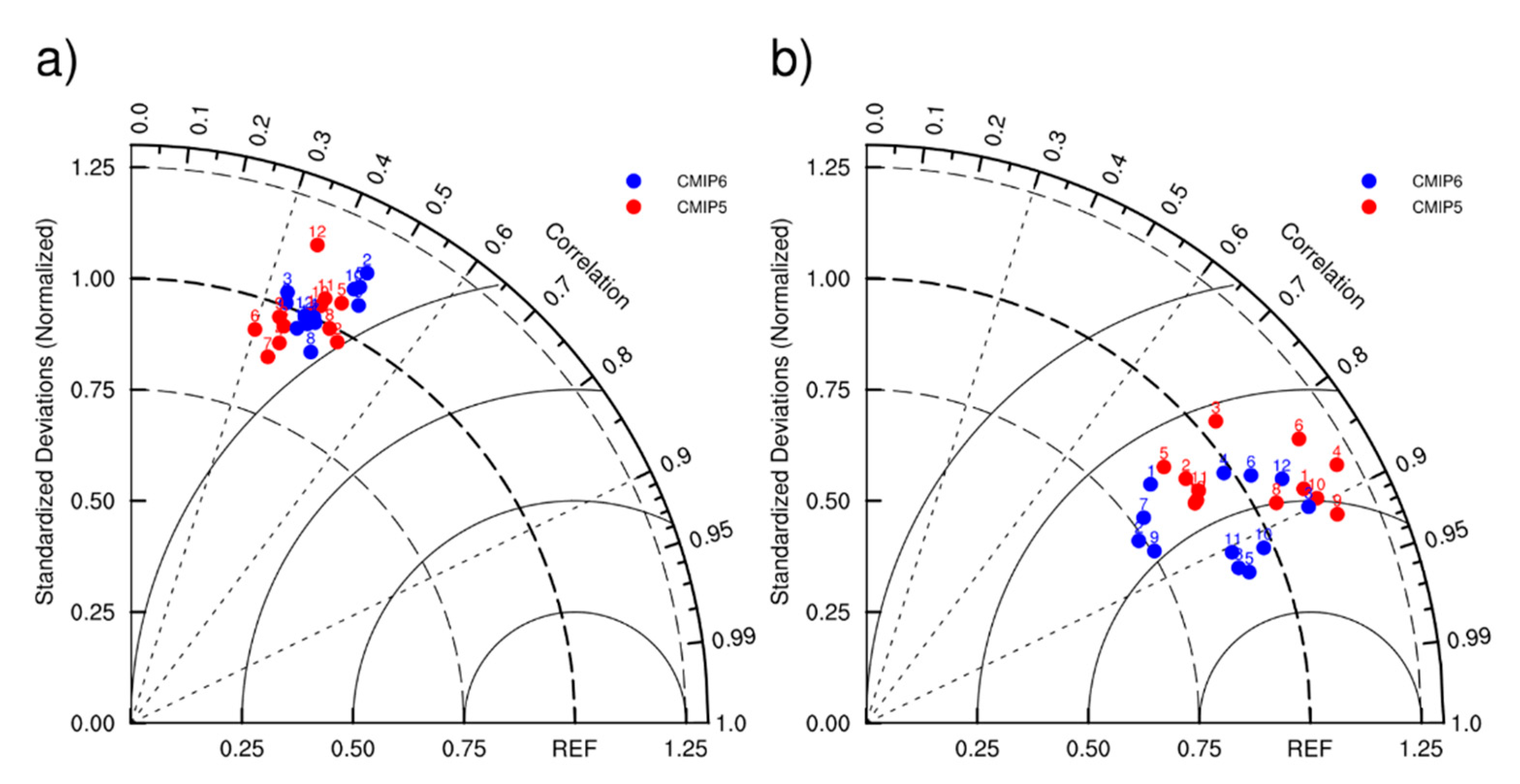
Figure 1. Taylor diagrams of (a) sea-level pressure (SLP) and (b) sea surface temperature (SST) simulated by the 12 CMIP5 models and 12 CMIP6 models with ERA5 as the reference data.
Atmosphere 11 00931 g001
Figure 2. Skill scores of the 12 CMIP5 models (blue) and 12 CMIP6 models (orange) for (a) SLP and (b) SST, respectively.
Atmosphere 11 00931 g002
Figure 3. Time-longitude (Hovmöller) diagrams for SLP monthly anomalies from the ERA5 dataset and selected models (contours at 0.5 hPa interval). (a) ERA5 (as reference data); (b) FIO-ESM-2-0 model (highest S score); (c) CMIP5 ensemble mean; (d) CESM1-CAM5 model (highest EOF1 time series correction in CMIP5); (e) CMIP6 ensemble mean and (f) CanESM5 model (highest EOF1 time series correction in CMIP6).
Atmosphere 11 00931 g003
Figure 4. Time series and spatial pattern for the first empirical orthogonal function (EOF) mode of SLP from the ERA5 dataset (a,b) and selected models (cg), with the explained percentage of variance given on the top right (5–95% percentile shaded). Models (cg) are the same as Figure 3bf.
Atmosphere 11 00931 g004
Figure 5. Spectra for bandpass-filtered first EOF time series of SLP from the ERA5 dataset (a) and selected models (red line is the red noise, and dashed line is the 5% and 95% confidence bounds). Models (bf) are the same as Figure 3bf.
Atmosphere 11 00931 g005
Figure 6. Same as Figure 3, but for SST (contours at 0.2 °C interval). (a) ERA5 (as reference data); (b) GFDL-CM4 model (highest S score); (c) CMIP5 ensemble mean; (d) ACCESS1.3 model (highest EOF1 time series correction in CMIP5); (e) CMIP6 ensemble mean and (f) CESM2 model (second highest EOF1 time series correction in CMIP6 with GFDL-CM4 as the highest).
Atmosphere 11 00931 g006
Figure 7. Time series and spatial pattern for the first EOF mode of SST from the ERA5 dataset (a,b) and selected models (cg), with the explained percentage of variance given on the top right (5–95% percentile shaded). Models (cg) are the same as Figure 6bf.
Atmosphere 11 00931 g007
Figure 8. Spectra for bandpass-filtered first EOF time series of SST from the ERA5 dataset (a) and selected models (red line is the red noise, and dashed line is the 5% and 95% confidence bounds). Models (bf) are the same as Figure 6bf.
Atmosphere 11 00931 g008
Table 1. Basic information for the 24 selected CMIP5 and CMIP6 models.
ProjectNo.Model NameInstitution and CountrySLP Spatial GridsSST Spatial Grids
CMIP51ACCESS1.3CSIRO-BOM, Australia192 × 145192 × 145
CMIP52CESM1-CAM5NSF-DOE-NCAR, USA288 × 192384 × 320
CMIP53CNRM-CM5CNRM-CERFACS, France256 × 128362 × 292
CMIP54FGOALS-g2LASG-CESS, China128 × 60360 × 196
CMIP55GFDL-CM3NOAA GFDL, USA144 × 90360 × 200
CMIP56GISS-E2-HNASA GISS, USA144 × 90144 × 90
CMIP57BCC-CSM1.1BCC, China128 × 64360 × 232
CMIP58CanESM2CCCMA, Canada128 × 64256 × 192
CMIP59FIO-ESMFIO, China128 × 64320 × 384
CMIP510GFDL-ESM2GNOAA GFDL, USA144 × 90360 × 210
CMIP511HadGEM2-CCMOHC, UK192 × 145360 × 216
CMIP512IPSL-CM5A-LRIPSL, France96 × 96182 × 149
CMIP61ACCESS-CM2CSIRO-ARCCSS, Australia192 × 144360 × 300
CMIP62CESM2NCAR, USA288 × 192320 × 384
CMIP63CNRM-CM6-1CNRM-CERFACS, France256 × 128362 × 294
CMIP64FGOALS-g3CAS, China180 × 80360 × 218
CMIP65GFDL-CM4NOAA-GFDL, USA360 × 1801440 × 1080
CMIP66GISS-E2-1-HNASA-GISS, USA144 × 90360 × 180
CMIP67BCC-CSM2-MRBCC, China320 × 160360 × 232
CMIP68CanESM5CCCMA, Canada128 × 64360 × 291
CMIP69FIO-ESM-2-0FIO-QLNM, China192 × 288320 × 384
CMIP610GFDL-ESM4NOAA-GFDL, USA288 × 180720 × 576
CMIP611HadGEM3-GC31-LLMOHC NERC, UK192 × 144360 × 330
CMIP612IPSL-CM6A-LRIPSL, France144 × 143362 × 332