Source–Receptor Relationships and Cluster Analysis of CO2, CH4, and CO Concentrations in West Africa: The Case of Lamto in Côte d’Ivoire

 , ,
, ,  , ,
, ,
Abstract
1. Introduction
2. Material Data and Method
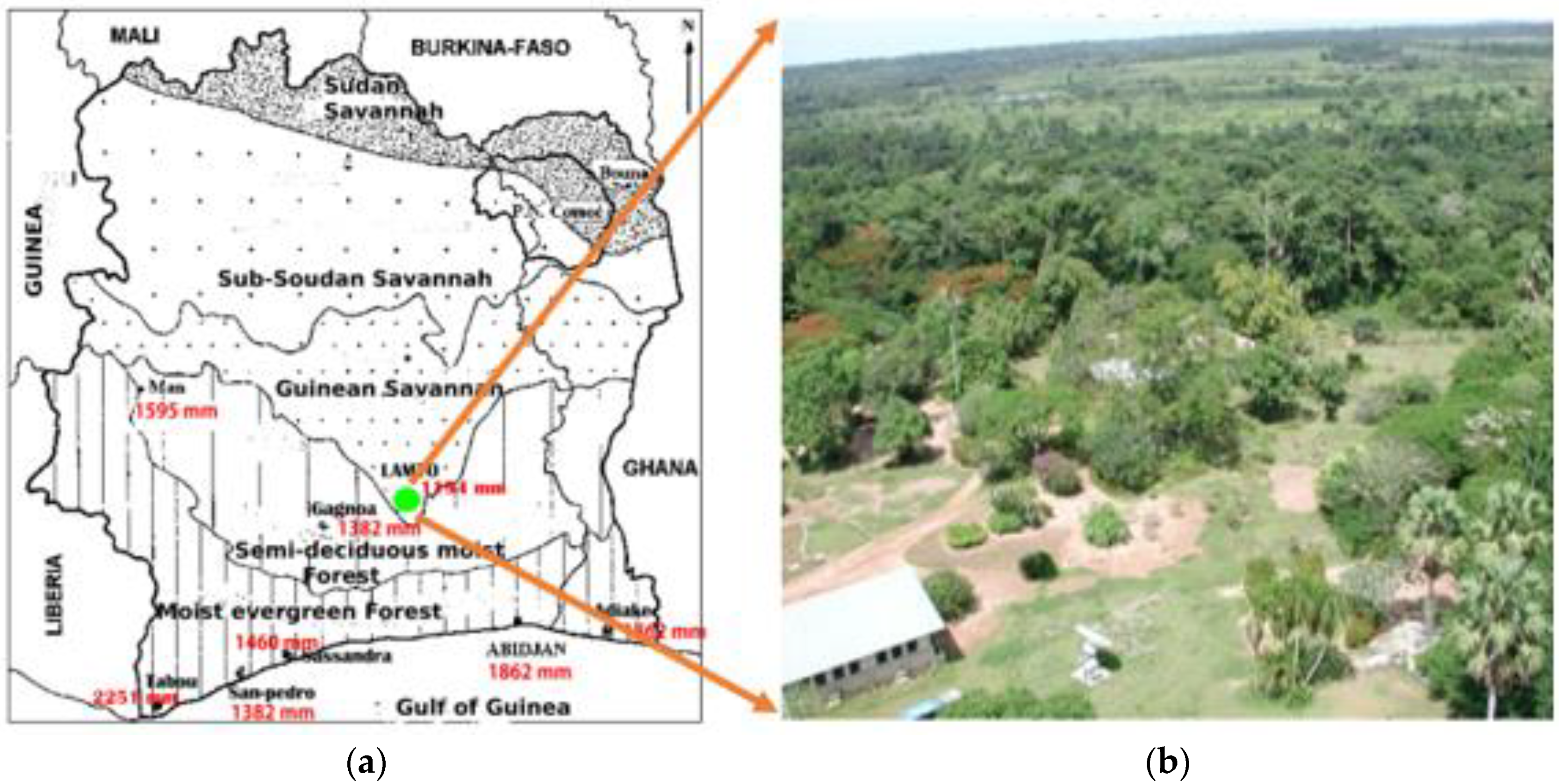
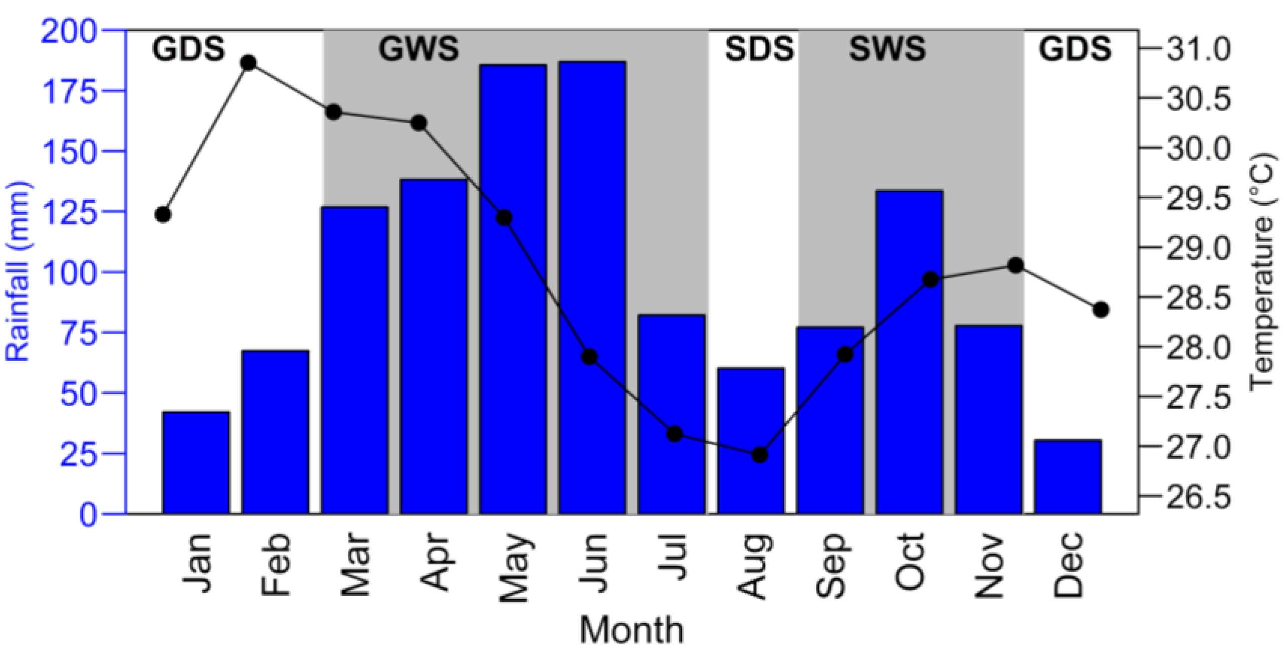
2.1. Site Description
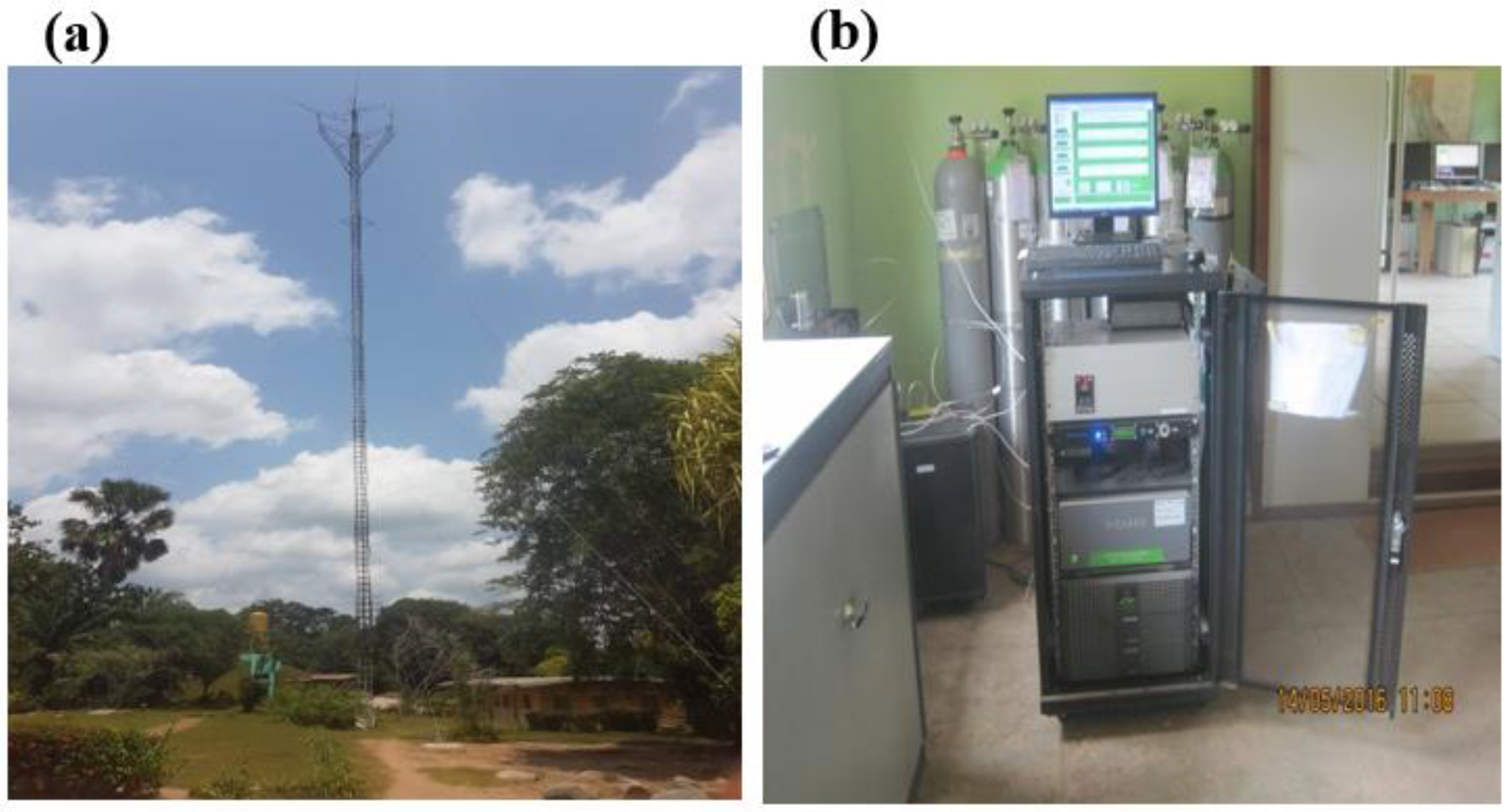
2.2. Measurement of CO2, CH4, and CO
2.3. FLEXPART Model
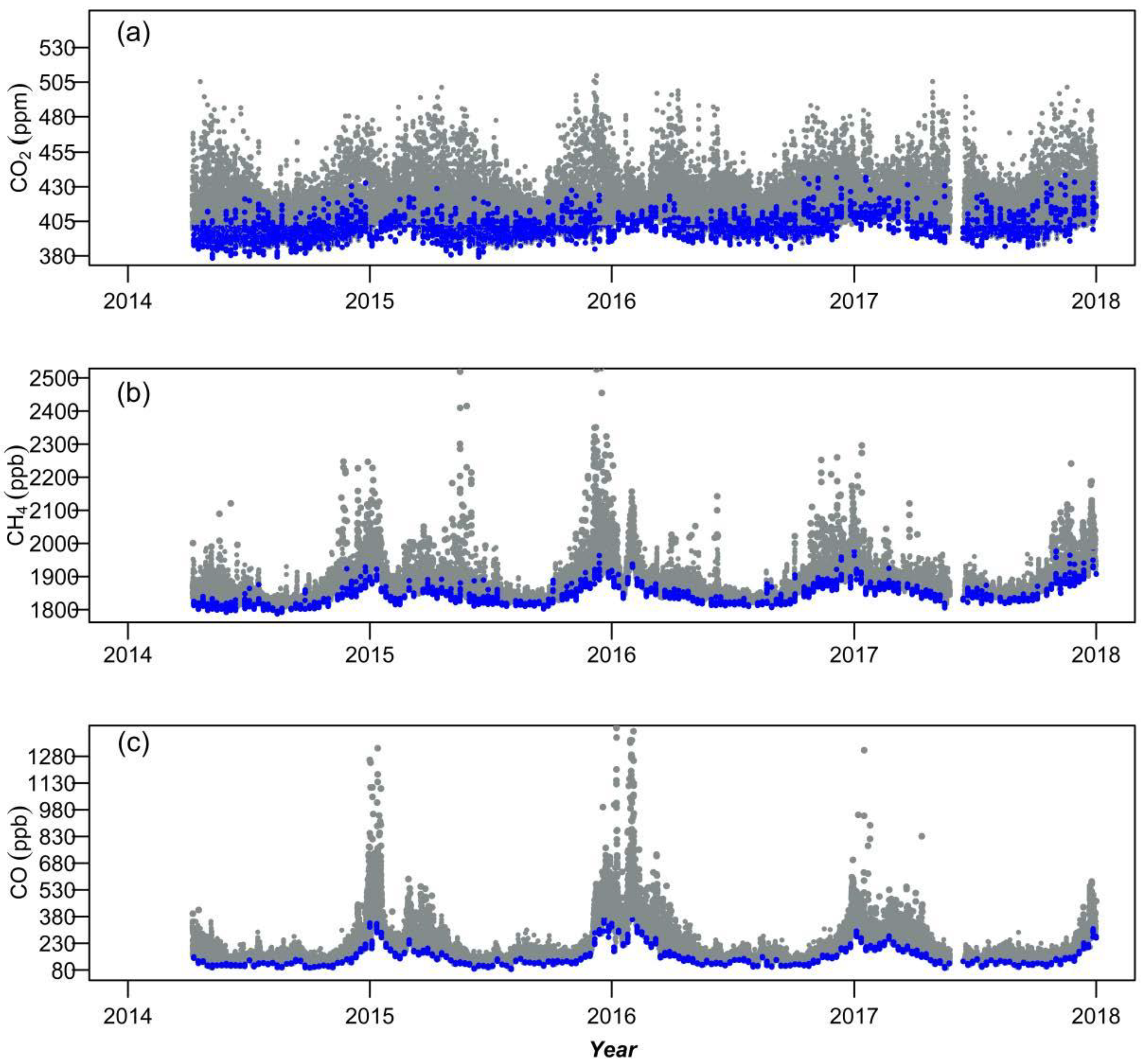
2.4. Time-Series and Background Signals of CO2, CH4, and CO
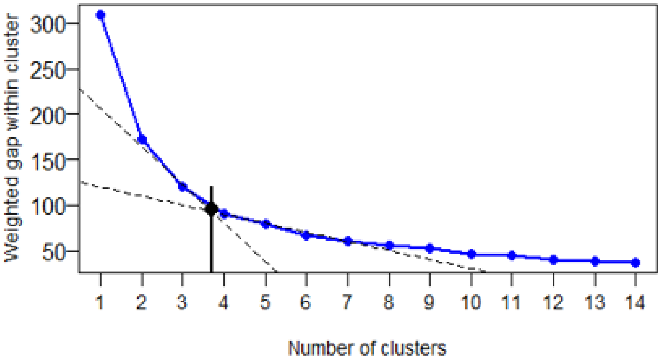
2.5. Clustering Method
3. Results
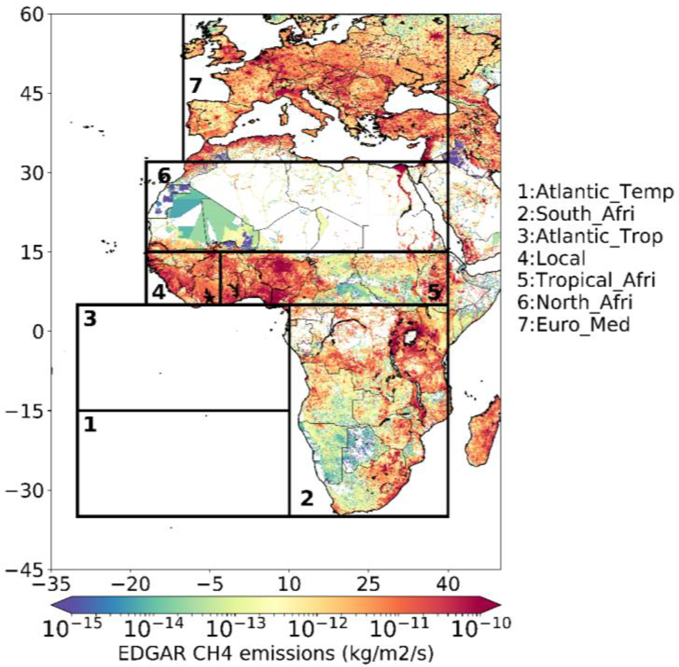
3.1. Correlations between PES over Each Region and CO2, CH4, and CO
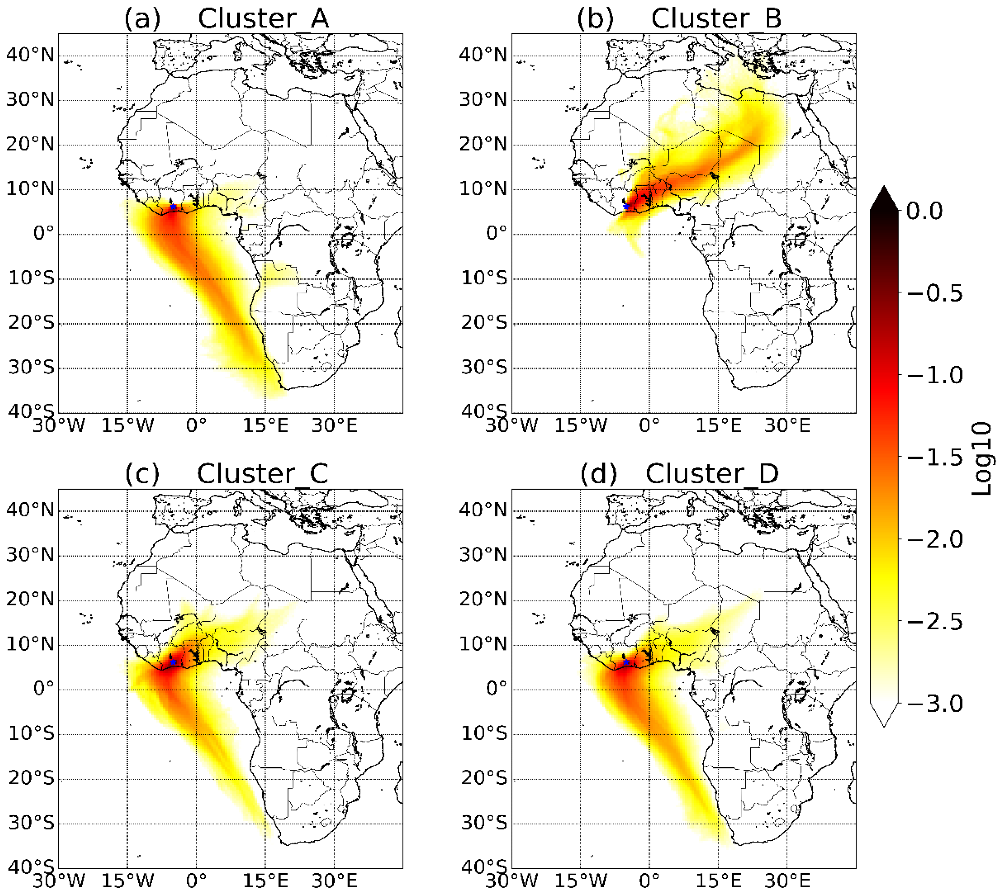
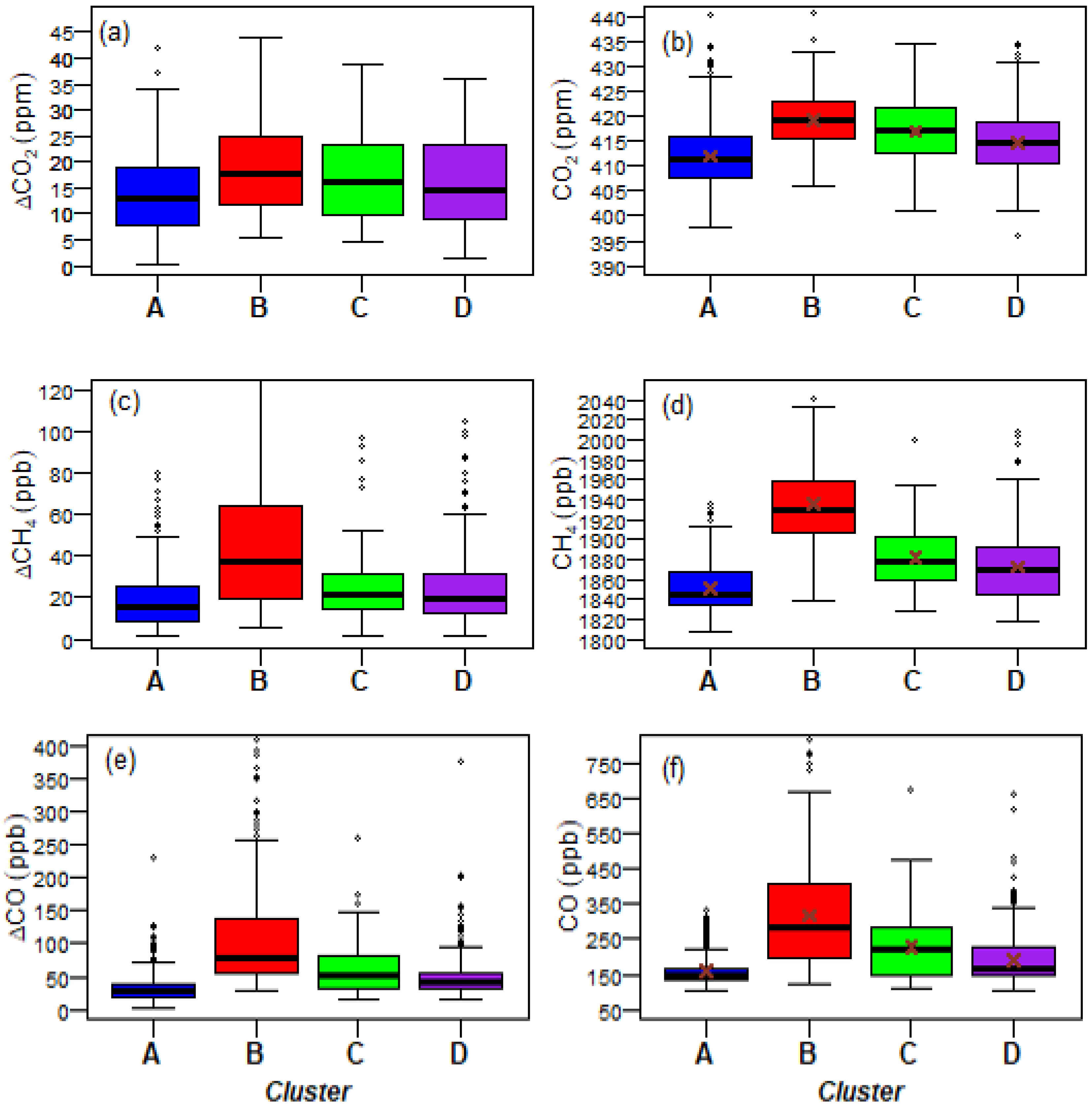
3.2. PES Clustering Applied to CO2, CH4, and CO Concentrations
- −
- Cluster A
- −
- Cluster B
- −
- Cluster C
- −
- Cluster D
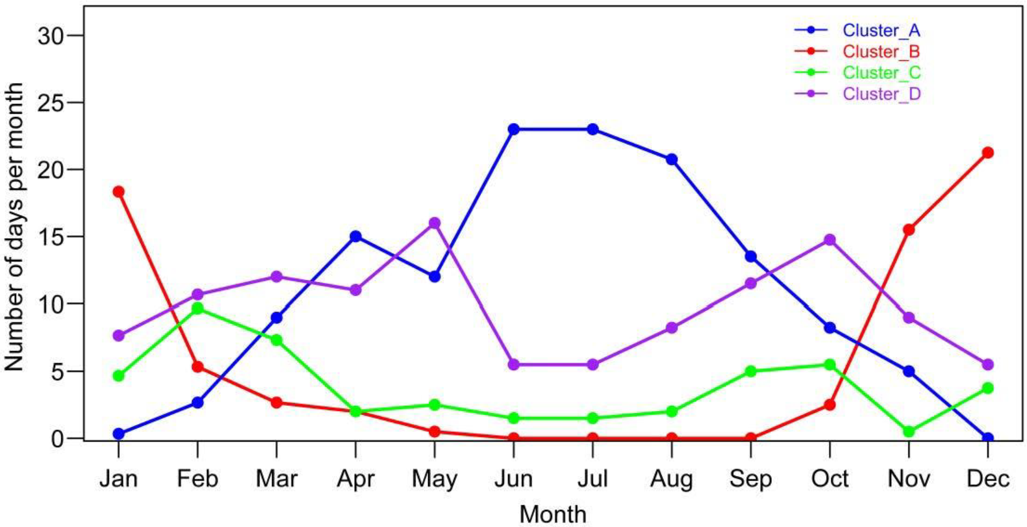
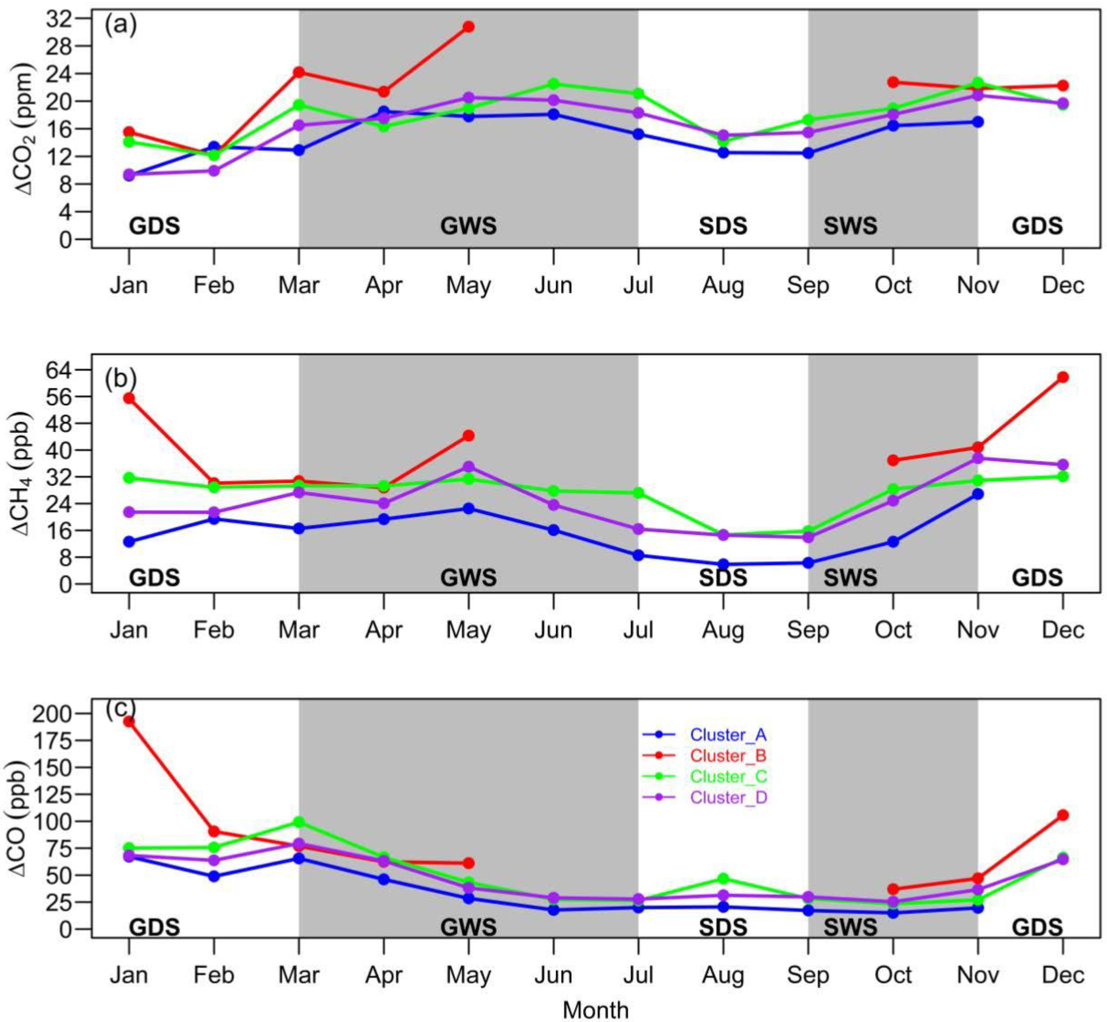
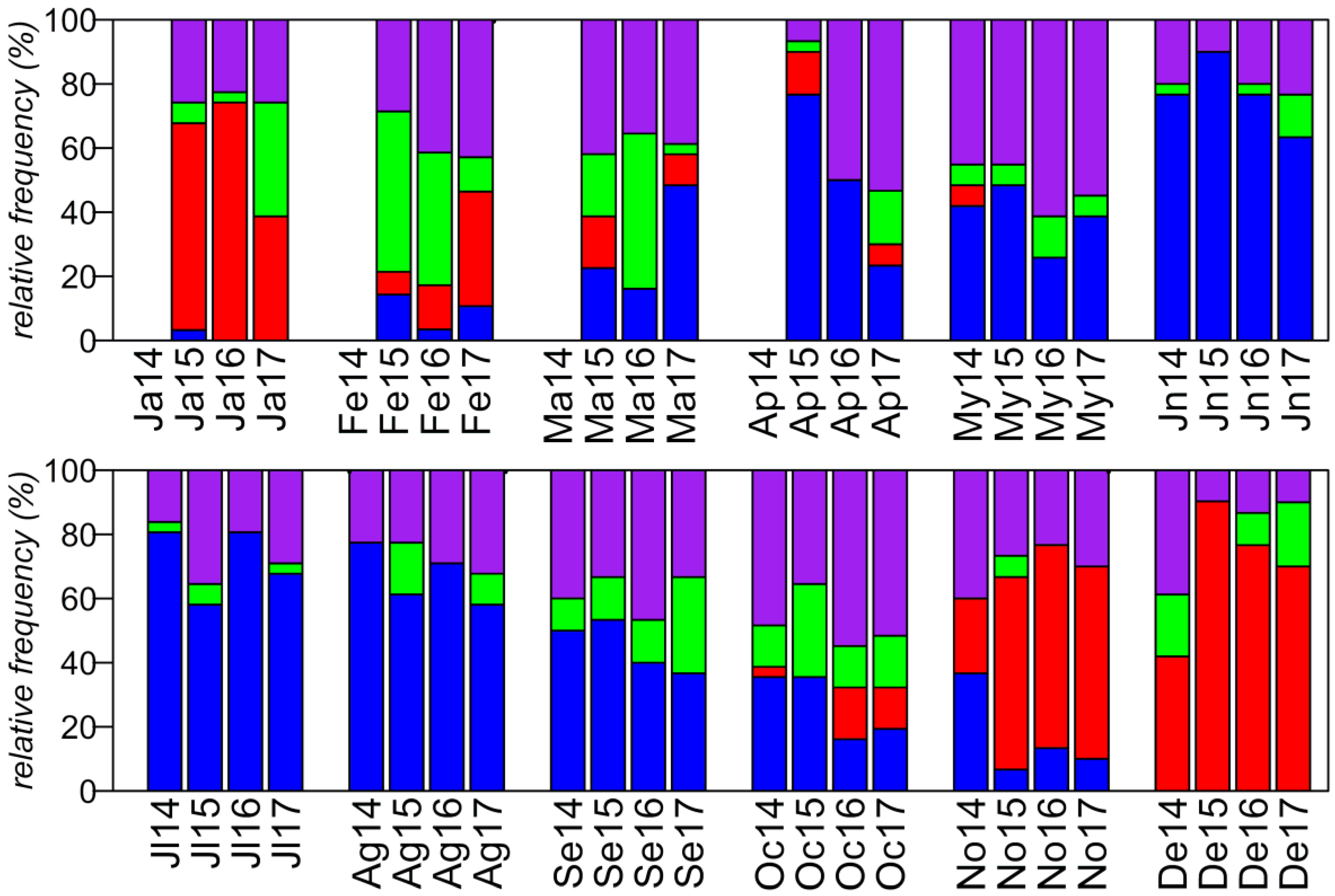
3.3. Seasonal Frequency of Clusters
3.4. Interannual Frequency of Clusters
4. Discussion
4.1. Impacts of Transport on the Concentrations of CO, CO2 and CH4
4.2. The Advantage of PES Clustering
5. Conclusions
- −
- Cluster A (≈37% of the retro-plumes) is clearly associated with oceanic and maritime air masses trajectories from the Souths.
- −
- Cluster B (≈21% of plumes) indicates continental origin.
- −
- Cluster C (≈11% of the retro- plumes) is associated with air mass advection from all directions including plumes of Sahelian origin.
- −
- Cluster D (≈31% of the retro-plumes) is attributed to the advection of air masses which have a significant oceanic signal.
Supplementary Materials
Author Contributions
Funding
Acknowledgments
Conflicts of Interest
Appendix A

| No. | Linear Models | R2 |
|---|---|---|
| (2) | 0.40 | |
| (3) | 0.74 | |
| (4) | 0.66 |

References
- IPCC. Climate Change 2014: Synthesis Report. Contribution of Working Groups I, II and III to the Fifth Assessment Report of the Intergovernmental Panel on Climate Change; Core Writing Team, Pachauri, R.K., Meyer, L.A., Eds.; IPCC: Geneva, Switzerland, 2014; p. 151. [Google Scholar]
- Ramaswamy, V. Radiative Forcing of Climate Change. In TAR Climate Change 2001: The Scientific Basis; Cambridge University Press: Cambridge, UK, 2001; Chapter 6; pp. 349–416. [Google Scholar]
- Niasse, M. Prévenir les conflits et promouvoir la coopération dans la gestion des fleuves transfrontaliers en Afrique de l’Ouest. Vertigo 2004. [Google Scholar] [CrossRef]
- Ciais, P.; Piao, S.-L.; Cadule, P.; Friedlingstein, P.; Chédin, A. Variability and recent trends in the African terrestrial carbon balance. Biogeosciences 2009, 6, 1935–1948. [Google Scholar] [CrossRef]
- Valentini, R.; Arneth, A.; Bombelli, A.; Castaldi, S.; Cazzolla Gatti, R.; Chevallier, F.; Ciais, P.; Grieco, E.; Hartmann, J.; Henry, M.; et al. The full greenhouse gases budget of Africa: Synthesis, uncertainties and vulnerabilities. Biogeosci. Discuss. 2013, 10, 8343–8413. [Google Scholar] [CrossRef]
- World Meteorological Organization. Proceedings of the 19th WMO/IAEA Meeting on Carbon Dioxide, Other Greenhouse Gases and Related Tracers Measurement Techniques (GGMT-2017), Dübendorf, Switzerland, 27–31 August 2017; GAW Report No. 242; World Meteorological Organization: Geneva, Switzerland, 2018; p. 134. [Google Scholar]
- Zimnoch, M.; Necki, J.; Chmura, L.; Jasek, A.; Jelen, D.; Galkowski, M.; Kuc, T.; Gorczyca, Z.; Bartyzel, J.; Rozanski, K. Quantification of carbon dioxide and methane emissions in urban areas: Source apportionment based on atmospheric observations. Mitig. Adapt. Strateg. Glob. Chang. 2019, 24, 1051–1071. [Google Scholar] [CrossRef]
- Ashbaugh, L.L. A Statistical Trajectory Technique for Determining Air Pollution Source Regions. J. Air Pollut. Control Assoc. 1983, 33, 1096–1098. [Google Scholar] [CrossRef]
- Ashbaugh, L.L.; Malm, W.C.; Sadeh, W.Z. A residence time probability analysis of sulfur concentrations at Grand Canyon National Park. Atmos. Environ. 1967 1985, 19, 1263–1270. [Google Scholar] [CrossRef]
- Cape, J.N.; Methven, J.; Hudson, L.E. The use of trajectory cluster analysis to interpret trace gas measurements at Mace Head, Ireland. Atmos. Environ. 2000, 34, 3651–3663. [Google Scholar] [CrossRef]
- Fiore, A.M.; Dentener, F.J.; Wild, O.; Cuvelier, C.; Schultz, M.G.; Hess, P.; Textor, C.; Schulz, M.; Doherty, R.M.; Horowitz, L.W.; et al. Multimodel estimates of intercontinental source-receptor relationships for ozone pollution. J. Geophys. Res. 2009, 114, D04301. [Google Scholar] [CrossRef]
- Paris, J.-D.; Stohl, A.; Ciais, P.; Nédélec, P.; Belan, B.D.; Arshinov, M.Y.; Ramonet, M. Source-receptor relationships for airborne measurements of CO2, CO and O3 above Siberia: A cluster-based approach. Atmos. Chem. Phys. 2010, 10, 1671–1687. [Google Scholar] [CrossRef]
- Fleming, Z.L.; Monks, P.S.; Manning, A.J. Review: Untangling the influence of air-mass history in interpreting observed atmospheric composition. Atmos. Res. 2012, 104–105, 1–39. [Google Scholar] [CrossRef]
- Buchholz, R.R.; Paton-Walsh, C.; Griffith, D.W.T.; Kubistin, D.; Caldow, C.; Fisher, J.A.; Deutscher, N.M.; Kettlewell, G.; Riggenbach, M.; Macatangay, R.; et al. Source and meteorological influences on air quality (CO, CH4 & CO2) at a Southern Hemisphere urban site. Atmos. Environ. 2016, 126, 274–289. [Google Scholar] [CrossRef]
- Riccio, A.; Giunta, G.; Chianese, E. The application of a trajectory classification procedure to interpret air pollution measurements in the urban area of Naples (Southern Italy). Sci. Total Environ. 2007, 376, 198–214. [Google Scholar] [CrossRef] [PubMed]
- Scott, G.M.; Diab, R.D. Forecasting Air Pollution Potential: A Synoptic Climatological Approach. J. Air Waste Manag. Assoc. 2000, 50, 1831–1842. [Google Scholar] [CrossRef]
- Ncipha, X.G.; Sivakumar, V.; Malahlela, O.E. The Influence of Meteorology and Air Transport on CO2 Atmospheric Distribution over South Africa. Atmosphere 2020, 11, 287. [Google Scholar] [CrossRef]
- Henne, S.; Klausen, J.; Junkermann, W.; Kariuki, J.M.; Aseyo, J.O.; Buchmann, B. Representativeness and climatology of carbon monoxide and ozone at the global GAW station Mt. Kenya in equatorial Africa. Atmos. Chem. Phys. 2008, 8, 3119–3139. [Google Scholar] [CrossRef]
- Almeida-Silva, M.; Almeida, S.M.; Cardoso, J.; Nunes, T.; Reis, M.A.; Chaves, P.C.; Pio, C.A. Characterization of the aeolian aerosol from Cape Verde by k 0-INAA and PIXE. J. Radioanal. Nucl. Chem. 2014, 300, 629–635. [Google Scholar] [CrossRef]
- Tiemoko, T.D.; Ramonet, M.; Yoroba, F.; Kouassi, K.B.; Kouadio, K.; Kazan, V.; Kaiser, C.; Truong, F.; Vuillemin, C.; Delmotte, M.; et al. Analysis of the temporal variability of CO2, CH4 and CO concentrations in West Africa: Case of the Lamto observatory in Côte d’Ivoire. Tellus B Chem. Phys. Meteorol. 2020, in press. [Google Scholar]
- Diawara, A.; Yoroba, F.; Kouadio, K.Y.; Kouassi, K.B.; Assamoi, E.M.; Diedhiou, A.; Assamoi, P. Climate Variability in the Sudano-Guinean Transition Area and Its Impact on Vegetation: The Case of the Lamto Region in Côte D’Ivoire. Adv. Meteorol. 2014, 2014, 1–11. [Google Scholar] [CrossRef][Green Version]
- Devineau, J.-L. Etude Quantitative des Forêts-Galeries de Lamto (Moyenne Côte d’Ivoire). Ph.D. Thesis, Université Pierre et Marie Curie-Paris VI, Paris, France, 1975. [Google Scholar]
- Cristofanelli, P.; Fierli, F.; Marinoni, A.; Calzolari, F.; Duchi, R.; Burkhart, J.; Stohl, A.; Maione, M.; Arduini, J.; Bonasoni, P. Influence of biomass burning and anthropogenic emissions on ozone, carbon monoxide and black carbon at the Mt. Cimone GAW-WMO global station (Italy, 2165 m a.s.l.). Atmos. Chem. Phys. 2013, 13, 15–30. [Google Scholar] [CrossRef]
- Stohl, A.; Huntrieser, H.; Richter, A.; Beirle, S.; Cooper, O.R.; Eckhardt, S.; Forster, C.; James, P.; Spichtinger, N.; Wenig, M.; et al. Rapid intercontinental air pollution transport associated with a meteorological bomb. Atmos. Chem. Phys. 2003, 3, 969–985. [Google Scholar] [CrossRef]
- Eneroth, K.; Kjellström, E.; Holmén, K. Interannual and seasonal variations in transport to a measuring site in western Siberia and their impact on the observed atmospheric CO2 mixing ratio: ATMOSPHERIC Transport and CO2. J. Geophys. Res. 2003, 108. [Google Scholar] [CrossRef]
- Tohjima, Y.; Kubo, M.; Minejima, C.; Mukai, H.; Tanimoto, H.; Ganshin, A.; Maksyutov, S.; Katsumata, K.; Machida, T.; Kita, K. Temporal changes in the emissions of CH4 and CO from China estimated from CH4/CO2 and CO/CO2 correlations observed at Hateruma Island. Atmos. Chem. Phys. 2014, 14, 1663–1677. [Google Scholar] [CrossRef]
- Markou, M.T.; Kassomenos, P. Cluster analysis of five years of back trajectories arriving in Athens, Greece. Atmos. Res. 2010, 98, 438–457. [Google Scholar] [CrossRef]
- Borge, R.; Lumbreras, J.; Vardoulakis, S.; Kassomenos, P.; Rodriguez, E. Analysis of long-range transport influences on urban PM10 using two-stage atmospheric trajectory clusters. Atmos. Environ. 2007, 41, 4434–4450. [Google Scholar] [CrossRef]
- Traub, M.; Fischer, H.; de Reus, M.; Kormann, R.; Heland, H.; Ziereis, H.; Schlager, H.; Holzinger, R.; Williams, J.; Warneke, C.; et al. Chemical characteristics assigned to trajectory clusters during the MINOS campaign. Atmos. Chem. Phys. 2003, 3, 459–468. [Google Scholar] [CrossRef]
- Stohl, A.; Hittenberger, M.; Wotawa, G. Validation of the lagrangian particle dispersion model FLEXPART against large-scale tracer experiment data. Atmos. Environ. 1998, 32, 4245–4264. [Google Scholar] [CrossRef]
- Hirdman, D.; Burkhart, J.F.; Sodemann, H.; Eckhardt, S.; Jefferson, A.; Quinn, P.K.; Sharma, S.; Ström, J.; Stohl, A. Long-term trends of black carbon and sulphate aerosol in the Arctic: Changes in atmospheric transport and source region emissions. Atmos. Chem. Phys. 2010, 10, 9351–9368. [Google Scholar] [CrossRef]
- Andreae, M.O.; Merlet, P. Emission of trace gases and aerosols from biomass burning. Glob. Biogeochem. Cycles 2001, 15, 955–966. [Google Scholar] [CrossRef]
- Paris, J.-D.; Ciais, P.; Nédélec, P.; Ramonet, M.; Belan, B.D.; Arshinov, M.Y.; Golitsyn, G.S.; Granberg, I.; Stohl, A.; Cayez, G.; et al. The YAK-AEROSIB transcontinental aircraft campaigns: New insights on the transport of CO2, CO and O3 across Siberia. Tellus B Chem. Phys. Meteorol. 2008, 60, 551–568. [Google Scholar] [CrossRef]
- Lin, X.; Indira, N.K.; Ramonet, M.; Delmotte, M.; Ciais, P.; Bhatt, B.C.; Reddy, M.V.; Angchuk, D.; Balakrishnan, S.; Jorphail, S.; et al. Long-lived atmospheric trace gases measurements in flask samples from three stations in India. Atmos. Chem. Phys. 2015, 15, 9819–9849. [Google Scholar] [CrossRef]
- Koffi, K.F.; N’Dri, A.B.; Lata, J.-C.; Konaté, S.; Srikanthasamy, T.; Konan, M.; Barot, S. Effect of fire regime on the grass community of the humid savanna of Lamto, Ivory Coast. J. Trop. Ecol. 2019, 35, 1–7. [Google Scholar] [CrossRef]
- Tiemoko, D.T.; Yoroba, F.; Diawara, A.; Kouadio, K.; Kouassi, B.K.; Yapo, A.L.M. Understanding the Local Carbon Fluxes Variations and Their Relationship to Climate Conditions in a Sub-Humid Savannah-Ecosystem during 2008-2015: Case of Lamto in Cote d’Ivoire. Atmos. Clim. Sci. 2020, 10, 186–205. [Google Scholar] [CrossRef][Green Version]
- Crosson, E.R. A cavity ring-down analyzer for measuring atmospheric levels of methane, carbon dioxide, and water vapor. Appl. Phys. B 2008, 92, 403–408. [Google Scholar] [CrossRef]
- Chen, H.; Winderlich, J.; Gerbig, C.; Hoefer, A.; Rella, C.W.; Crosson, E.R.; Van Pelt, A.D.; Steinbach, J.; Kolle, O.; Beck, V.; et al. High-accuracy continuous airborne measurements of greenhouse gases (CO2 and CH4) using the cavity ring-down spectroscopy (CRDS) technique. Atmos. Meas. Tech. 2010, 3, 375–386. [Google Scholar] [CrossRef]
- Filges, A.; Gerbig, C.; Chen, H.; Franke, H.; Klaus, C.; Jordan, A. The IAGOS-core greenhouse gas package: A measurement system for continuous airborne observations of CO2, CH4, H2O and CO. Tellus B Chem. Phys. Meteorol. 2015, 67, 27989. [Google Scholar] [CrossRef]
- Van der Werf, G.R.; Randerson, J.T.; Giglio, L.; van Leeuwen, T.T.; Chen, Y.; Rogers, B.M.; Mu, M.; van Marle, M.J.E.; Morton, D.C.; Collatz, G.J.; et al. Global fire emissions estimates during 1997–2016. Earth Syst. Sci. Data 2017, 9, 697–720. [Google Scholar] [CrossRef]
- Crippa, M.; Solazzo, E.; Huang, G.; Guizzardi, D.; Koffi, E.; Muntean, M.; Schieberle, C.; Friedrich, R.; Janssens-Maenhout, G. High resolution temporal profiles in the Emissions Database for Global Atmospheric Research. Sci. Data 2020, 7, 121. [Google Scholar] [CrossRef]
- Stohl, A.; Aamaas, B.; Amann, M.; Baker, L.H.; Bellouin, N.; Berntsen, T.K.; Boucher, O.; Cherian, R.; Collins, W.; Daskalakis, N.; et al. Evaluating the climate and air quality impacts of short-lived pollutants. Atmos. Chem. Phys. 2015, 15, 10529–10566. [Google Scholar] [CrossRef]
- Seibert, P.; Frank, A. Source-receptor matrix calculation with a Lagrangian particle dispersion model in backward mode. Atmos. Chem. Phys. 2004, 4, 51–63. [Google Scholar] [CrossRef]
- Stohl, A.; Forster, C.; Frank, A.; Seibert, P.; Wotawa, G. Technical note: The Lagrangian particle dispersion model FLEXPART version 6.2. Atmos. Chem. Phys. 2005, 5, 2461–2474. [Google Scholar] [CrossRef]
- Berchet, A.; Paris, J.-D.; Ancellet, G.; Law, K.S.; Stohl, A.; Nédélec, P.; Arshinov, M.Y.; Belan, B.D.; Ciais, P. Tropospheric ozone over Siberia in spring 2010: Remote influences and stratospheric intrusion. Tellus B Chem. Phys. Meteorol. 2013, 65, 19688. [Google Scholar] [CrossRef]
- Aryee, J.N.A.; Amekudzi, L.K.; Preko, K.; Atiah, W.A.; Danuor, S.K. Estimation of planetary boundary layer height from radiosonde profiles over West Africa during the AMMA field campaign: Intercomparison of different methods. Sci. Afr. 2020, 7, e00228. [Google Scholar] [CrossRef]
- Kalthoff, N.; Lohou, F.; Brooks, B.; Jegede, G.; Adler, B.; Babić, K.; Dione, C.; Ajao, A.; Amekudzi, L.K.; Aryee, J.N.A.; et al. An overview of the diurnal cycle of the atmospheric boundary layer during the West African monsoon season: Results from the 2016 observational campaign. Atmos. Chem. Phys. 2018, 18, 2913–2928. [Google Scholar] [CrossRef]
- Fletcher, S.E.M.; Schaefer, H. Rising methane: A new climate challenge. Science 2019, 364, 932–933. [Google Scholar] [CrossRef]
- Denjean, C.; Bourrianne, T.; Burnet, F.; Mallet, M.; Maury, N.; Colomb, A.; Dominutti, P.; Brito, J.; Dupuy, R.; Sellegri, K.; et al. Overview of aerosol optical properties over southern West Africa from DACCIWA aircraft measurements. Atmos. Chem. Phys. 2020, 20, 4735–4756. [Google Scholar] [CrossRef]
- Super, I.; van der Gon, D.H.A.C.; van der Molen, M.K.; Sterk, H.A.M.; Hensen, A.; Peters, W. A multi-model approach to monitor emissions of CO2 and CO in an urban-industrial complex. Atmos. Chem. Phys. Discuss. 2017, 17, 13297–13316. [Google Scholar] [CrossRef]
- Oney, B.; Gruber, N.; Henne, S.; Leuenberger, M.; Brunner, D. A CO-based method to determine the regional biospheric signal in atmospheric CO2. Tellus B Chem. Phys. Meteorol. 2017, 69, 1353388. [Google Scholar] [CrossRef]
- Anderberg, M.R. Cluster-Analysis for Applications; Academic Press: New York, NY, USA, 1973. [Google Scholar]
- McQueen, J.B. Some methods for classification and analysis of multivariate observations. In Proceedings of the 5th Berkeley Symposium on Mathematical, Statistics and Probability, Berkeley, CA, USA, 18–21 July 1967; Volume 1. [Google Scholar]
- Ding, C.; He, X. K-Means Clustering via Principal Component Analysis. In ICML ’04, Proceedings of the Twenty-First International Conference on Machine Learning, New York, NY, USA, July 2004; ACM Press: Banff, AB, Canada, 2004; p. 29. [Google Scholar] [CrossRef]
- EDGAR v5.0 EC-JRC/PBL (European Commission, Joint Research Centre/Netherlands Environmental Assessment Agency). Emission Database for Global Atmospheric Research (EDGAR); Nature Scientific Data, EDGARv5. 2019. Available online: https://edgar.jrc.ec.europa.eu/overview.php?v=50_GHG (accessed on 23 August 2020). [CrossRef]
- Kalkstein, L.S.; Tan, G.; Skindlov, J.A. An evaluation of three clustering procedures for use in synoptic. J. Climatol. Appl. Meteorol. 1987, 26, 717–730. [Google Scholar] [CrossRef]
- Yan, M. Methods of Determining the Number of Clusters in a Data Set and a New Clustering Criterion. Ph.D. Thesis, Virginia Polytechnic and State University, Blacksburg, VA, USA, 2005. [Google Scholar]
- Jorba, O.; Rocadenbosch, F.; Baldasano, J. Cluster Analysis of 4-Day Back Trajectories Arriving in the Barcelona Area, Spain, from 1997 to 2002. J. Appl. Meteorol. 2004, 43, 887–901. [Google Scholar] [CrossRef]
- Pisso, I.; Sollum, E.; Grythe, H.; Kristiansen, N.I.; Cassiani, M.; Eckhardt, S.; Arnold, D.; Morton, D.; Thompson, R.L.; Groot Zwaaftink, C.D.; et al. The Lagrangian particle dispersion model FLEXPART version 10.4. Geosci. Model Dev. 2019, 12, 4955–4997. [Google Scholar] [CrossRef]
- Paris, J.D.; Stohl, A.; Ciais, P.; Ramonet, M.; Nédélec, P. Relations source-récepteur transcontinentales identifiées avec un modèle Lagrangien de dispersion et une analyse en clusters. Pollut. Atmos. Clim. Sant. Soc. 2010, Special, 143–148. [Google Scholar]
- Bonsang, B.; Boissard, C.; Le Cloarec, M.F.; Rudolph, J.; Lacaux, J.P. Methane, carbon monoxide and light non-methane hydrocarbon emissions from African savanna burnings during the FOS/DECAFE experiment. J. Atmos. Chem. 1995, 22, 149–162. [Google Scholar] [CrossRef][Green Version]
- Crippa, M.; Guizzardi, D.; Muntean, M.; Schaaf, E.; Dentener, F.; van Aardenne, J.A.; Monni, S.; Doering, U.; Olivier, J.G.J.; Pagliari, V.; et al. Gridded Emissions of Air Pollutants for the period 1970-2012 withinEDGAR v4.3.2. Earth Syst. Sci. Data Discuss. 2018. [Google Scholar] [CrossRef]
- Freitag, H.; Ferguson, P.; Dubois, K.; Hayford, E.; Vonvordzogbe, V.; Veizer, J. Water and carbon fluxes from savanna ecosystems of the Volta River watershed, West Africa. Glob. Planet. Chang. 2008, 61, 3–14. [Google Scholar] [CrossRef]
- Pedruzo-Bagazgoitia, X.; de Roode, S.R.; Adler, B.; Babić, K.; Dione, C.; Kalthoff, N.; Lohou, F.; Lothon, M.; de Arellano, J.V.-G. The diurnal stratocumulus-to-cumulus transition over land in southern West Africa. Atmos. Chem. Phys. 2020, 20, 2735–2754. [Google Scholar] [CrossRef]
- Simonson, R.W. Airborne dust and its significance to soils. Geoderma 1995, 65, 1–43. [Google Scholar] [CrossRef]
- Scholes, R.J.; Archibald, S.; von Maltitz, G. Emissions from fire in sub-saharan Africa: The magnitude of sources, their variability and uncertainty. Glob. Environ. Res. 2011, 53–63. [Google Scholar]
- Jonquières, I.; Marenco, A.; Maalej, A.; Rohrer, F. Study of ozone formation and transatlantic transport from biomass burning emissions over West Africa during the airborne Tropospheric Ozone Campaigns TROPOZ I and TROPOZ II. J. Geophys. Res. 1998, 103, 19059–19073. [Google Scholar] [CrossRef]
- Edwards, D.P. Tropospheric ozone over the tropical Atlantic: A satellite perspective. J. Geophys. Res. 2003, 108, 4237. [Google Scholar] [CrossRef]
- Pradier, S.; Attié, J.-L.; Chong, M.; Escobar, J.; Peuch, V.-H.; Lamarque, J.-F.; Khattatov, B.; Edwards, D. Evaluation of 2001 springtime CO transport over West Africa using MOPITT CO measurements assimilated in a global chemistry transport model. Tellus B Chem. Phys. Meteorol. 2006, 58, 163–176. [Google Scholar] [CrossRef]
- Agier, L.; Deroubaix, A.; Martiny, N.; Yaka, P.; Djibo, A.; Broutin, H. Seasonality of meningitis in Africa and climate forcing: Aerosols stand out. J. R. Soc. Interface 2013, 10, 20120814. [Google Scholar] [CrossRef] [PubMed]
- Salvador, P.; Almeida, S.M.; Cardoso, J.; Almeida-Silva, M.; Nunes, T.; Cerqueira, M.; Alves, C.; Reis, M.A.; Chaves, P.C.; Artíñano, B.; et al. Composition and origin of PM 10 in Cape Verde: Characterization of long-range transport episodes. Atmos. Environ. 2016, 127, 326–339. [Google Scholar] [CrossRef]
- Sunnu, A.; Afeti, G.; Resch, F. A long-term experimental study of the Saharan dust presence in West Africa. Atmos. Res. 2008, 87, 13–26. [Google Scholar] [CrossRef]
- Touré, N.E.; Konaré, A.; Silué, S. Intercontinental Transport and Climatic Impact of Saharan and Sahelian Dust. Adv. Meteorol. 2012, 2012, 1–14. [Google Scholar] [CrossRef]
- Burton, R.R.; Devine, G.M.; Parker, D.J.; Chazette, P.; Dixon, N.; Flamant, C.; Haywood, J.M. The Harmattan over West Africa: Nocturnal structure and frontogenesis. Q. J. R. Meteorol. Soc. 2013, 139, 1364–1373. [Google Scholar] [CrossRef]
- D’Almeida, G.A. A model for Saharan dust transport. J. Clim. Appl. Meteor. 1986, 25, 903–916. [Google Scholar] [CrossRef]
- Karam, D.B. Mécanismes de Soulèvement D’aérosols Désertiques en Afrique de l’Ouest. Ph.D. Thesis, Université Pierre et Marie Curie Paris-VI, Paris, France, 2008. [Google Scholar]
- Lan, L.; Ghasemifard, H.; Yuan, Y.; Hachinger, S.; Zhao, X.; Bhattacharjee, S.; Bi, X.; Bai, Y.; Menzel, A.; Chen, J. Assessment of Urban CO2 Measurement and Source Attribution in Munich Based on TDLAS-WMS and Trajectory Analysis. Atmosphere 2020, 11, 58. [Google Scholar] [CrossRef]
- Moody, J.L.; Galloway, J.N. Quantifying the relationship between atmospheric transport and the chemical composition of precipitation on Bermuda. Tellus B Chem. Phys. Meteorol. 1988, 40, 463–479. [Google Scholar] [CrossRef]
- Brankov, E.; Rao, S.T.; Porter, P.S. A trajectory-clustering-correlation methodology for examining the long-range transport of air pollutants. Atmos. Environ. 1998, 32, 1525–1534. [Google Scholar] [CrossRef]
- Denjean, C.; Bourrianne, T.; Burnet, F.; Mallet, M.; Maury, N.; Colomb, A.; Dominutti, P.; Brito, J.; Dupuy, R.; Sellegri, K.; et al. Light absorption properties of aerosols over Southern West Africa, Aerosols/Field Measurements/Troposphere/Physics (physical properties and processes). Atmos. Chem. Phys. 2019. [Google Scholar] [CrossRef]


| Regions | CO2 | CH4 | CO | |||
|---|---|---|---|---|---|---|
| Pear (r) a | Ken (tau) b | Pear (r) a | Ken (tau) b | Pear (r) a | Ken (tau) b | |
| Local | 0.12 | 0.07 | −0.01 | 0.00 | 0.00 | 0.06 |
| Atlantic_Tem | −0.50 | −0.40 | −0.56 | −0.54 | −0.49 | −0.54 |
| Atlantic_Trop | −0.15 | −0.25 | −0.21 | −0.35 | −0.09 | −0.16 |
| Tropical_Afri | 0.52 | 0.39 | 0.82 | 0.64 | 0.66 | 0.46 |
| South_Afri | −0.22 | −0.25 | −0.40 | −0.38 | −0.41 | −0.43 |
| North_Afri | 0.38 | 0.37 | 0.72 | 0.61 | 0.75 | 0.49 |
| Euro_Med | 0.27 | 0.30 | 0.59 | 0.45 | 0.66 | 0.43 |
| Clusters | CO2 | CH4 | CO | |||
|---|---|---|---|---|---|---|
| Pear (r) a | Ken (tau) b | Pear (r) a | Ken (tau) b | Pear (r) a | Ken (tau) b | |
| Cluster A | −0.07 | −0.04 | 0.01 | −0.005 | −0.11 | −0.03 |
| Cluster B | 0.47 | 0.39 | 0.74 | 0.61 | 0.76 | 0.64 |
| Cluster C | 0.31 | 0.21 | 0.61 | 0.45 | 0.54 | 0.39 |
| Cluster D | 0.20 | 0.16 | 0.60 | 0.38 | 0.51 | 0.20 |
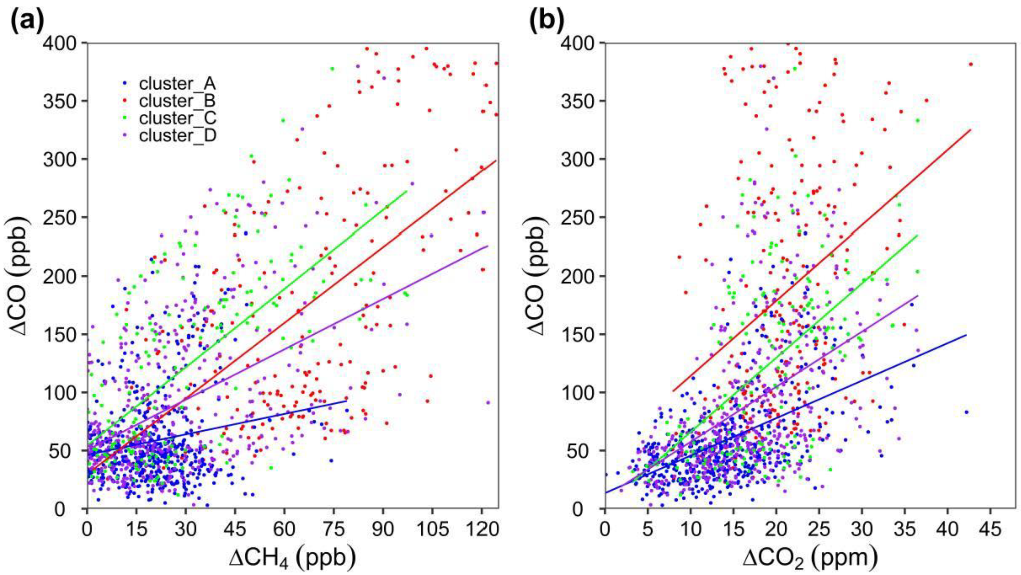
| Clusters | ΔCO/ΔCH4 | ΔCO/ΔCO2 | ||
|---|---|---|---|---|
| Slope (ppb/ppb) | Corr (r) * | Slope (ppb/ppm) | Corr (r) * | |
| Cluster A | 1.59 | 0.26 | 3.22 | 0.57 |
| Cluster B | 4.16 | 0.70 | 9.97 | 0.43 |
| Cluster C | 4.48 | 0.77 | 8.16 | 0.63 |
| Cluster D | 3.15 | 0.55 | 4.85 | 0.51 |
© 2020 by the authors. Licensee MDPI, Basel, Switzerland. This article is an open access article distributed under the terms and conditions of the Creative Commons Attribution (CC BY) license (http://creativecommons.org/licenses/by/4.0/).
Share and Cite
Tiemoko, D.T.; Yoroba, F.; Paris, J.-D.; Diawara, A.; Berchet, A.; Pison, I.; Riandet, A.; Ramonet, M. Source–Receptor Relationships and Cluster Analysis of CO2, CH4, and CO Concentrations in West Africa: The Case of Lamto in Côte d’Ivoire. Atmosphere 2020, 11, 903. https://doi.org/10.3390/atmos11090903
Tiemoko DT, Yoroba F, Paris J-D, Diawara A, Berchet A, Pison I, Riandet A, Ramonet M. Source–Receptor Relationships and Cluster Analysis of CO2, CH4, and CO Concentrations in West Africa: The Case of Lamto in Côte d’Ivoire. Atmosphere. 2020; 11(9):903. https://doi.org/10.3390/atmos11090903
Chicago/Turabian StyleTiemoko, Dro Touré, Fidèle Yoroba, Jean-Daniel Paris, Adama Diawara, Antoine Berchet, Isabelle Pison, Aurélie Riandet, and Michel Ramonet. 2020. "Source–Receptor Relationships and Cluster Analysis of CO2, CH4, and CO Concentrations in West Africa: The Case of Lamto in Côte d’Ivoire" Atmosphere 11, no. 9: 903. https://doi.org/10.3390/atmos11090903
APA StyleTiemoko, D. T., Yoroba, F., Paris, J.-D., Diawara, A., Berchet, A., Pison, I., Riandet, A., & Ramonet, M. (2020). Source–Receptor Relationships and Cluster Analysis of CO2, CH4, and CO Concentrations in West Africa: The Case of Lamto in Côte d’Ivoire. Atmosphere, 11(9), 903. https://doi.org/10.3390/atmos11090903