Urban-Scale NO2 Prediction with Sensors Aboard Bicycles: A Comparison of Statistical Methods Using Synthetic Observations

 , and
, and
Abstract
1. Introduction
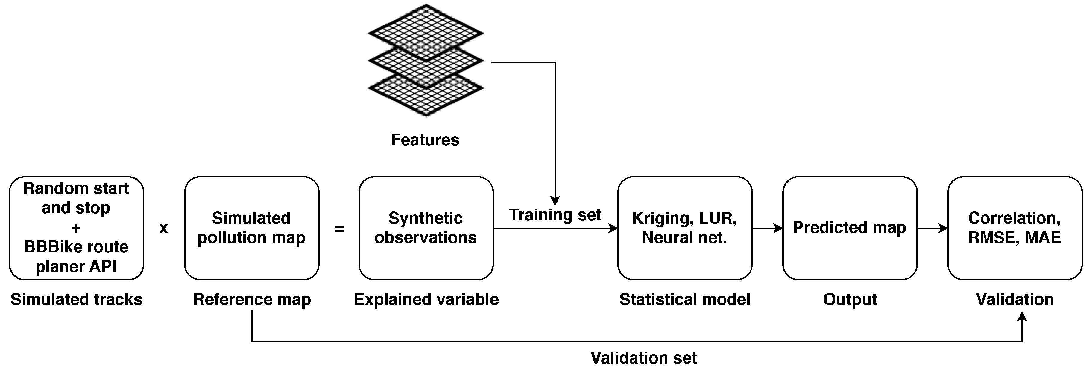
2. Method
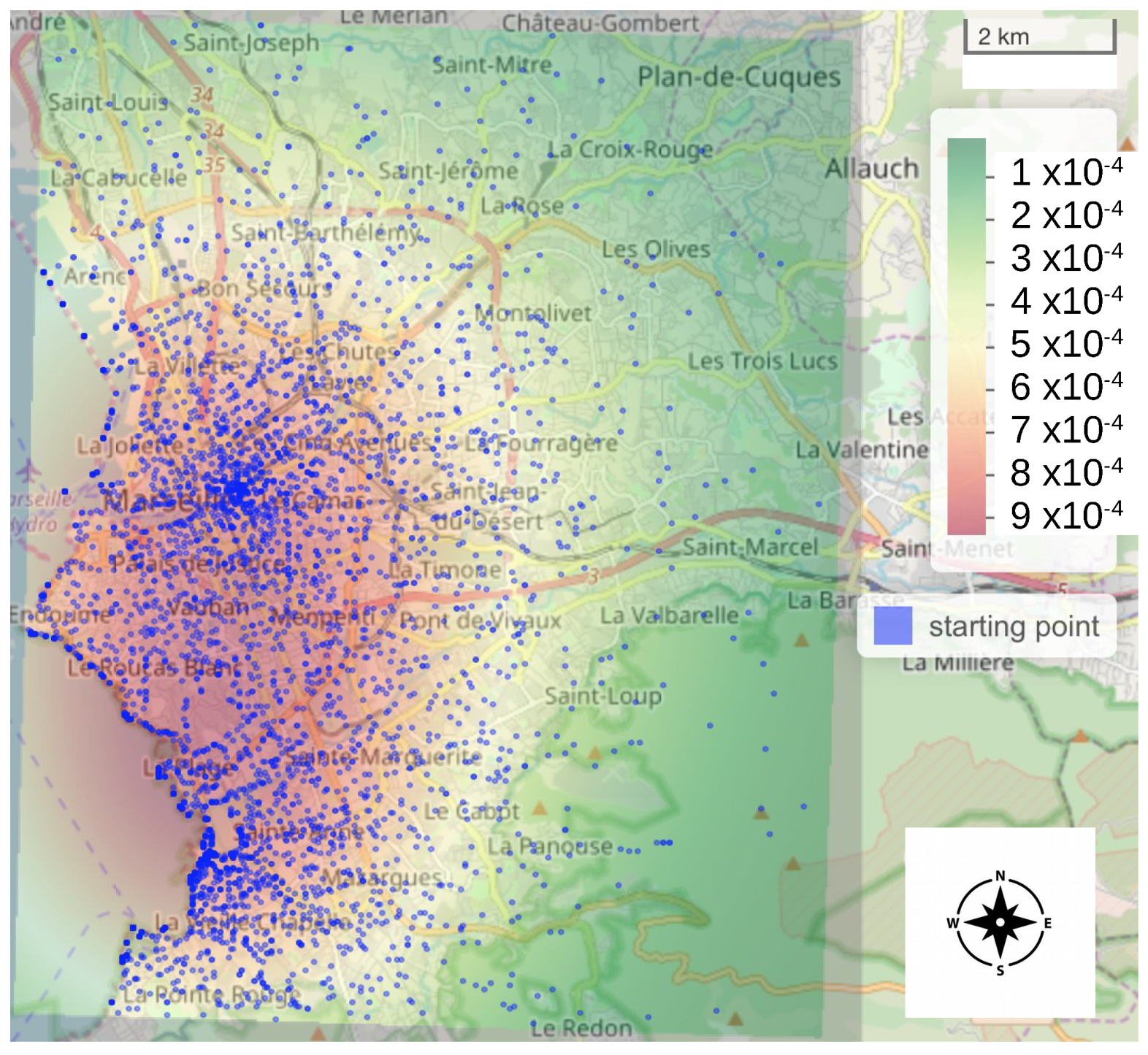
2.1. Study Area
2.2. Synthetic Observations
2.2.1. Air Quality Simulations
2.2.2. Geographical Features
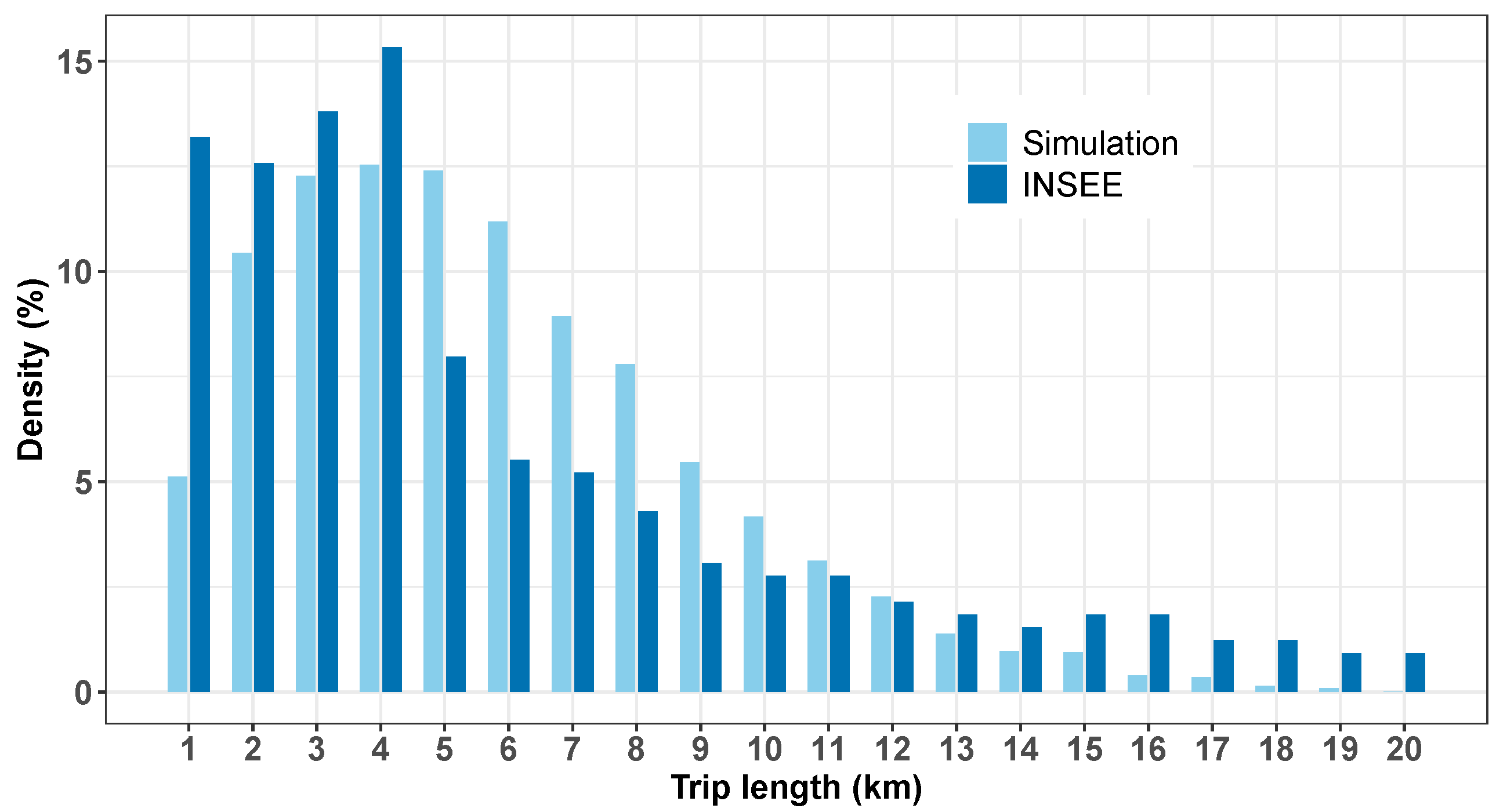
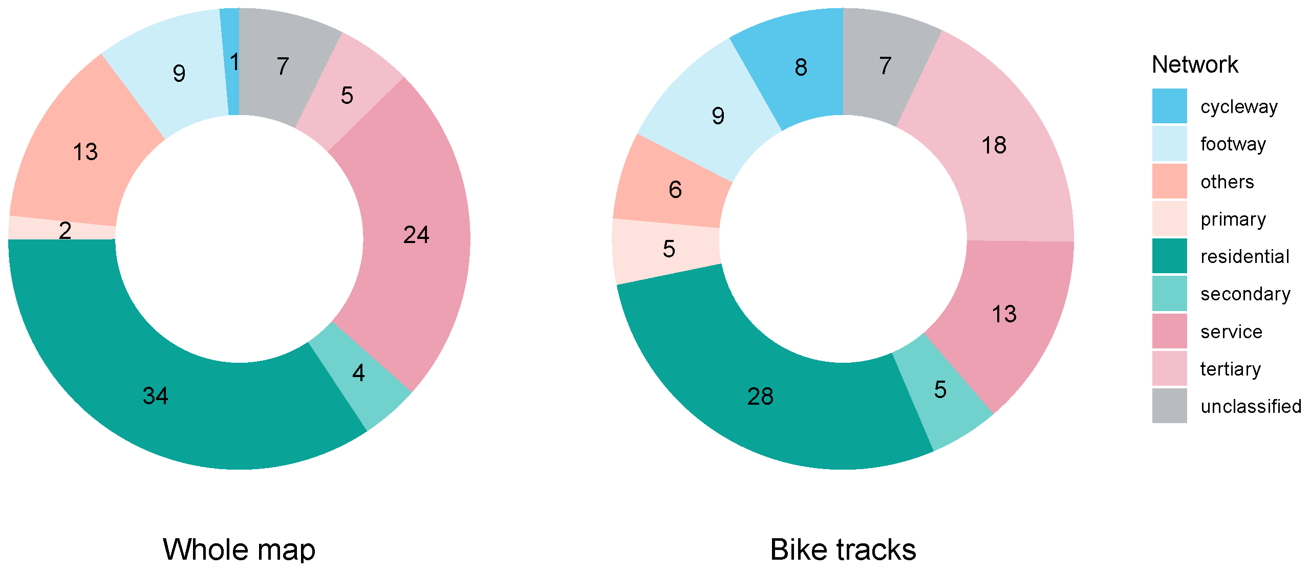
2.2.3. Simulated Bike Tracks
2.3. Statistical Models
2.3.1. Kriging
2.3.2. Generalized Additive Model
2.3.3. Artificial Neural Network
2.4. Evaluation Procedure
3. Results
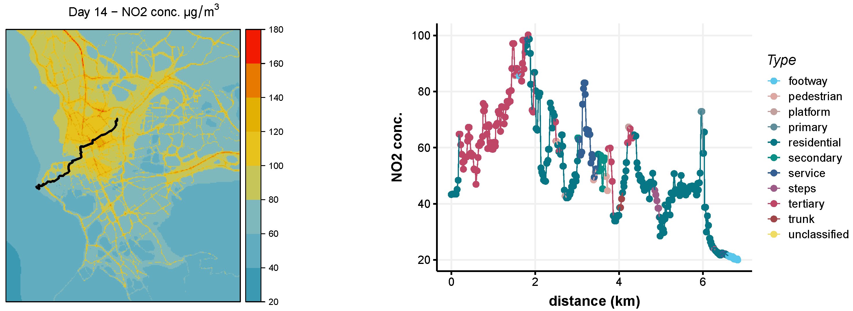
3.1. Synthetic Observations
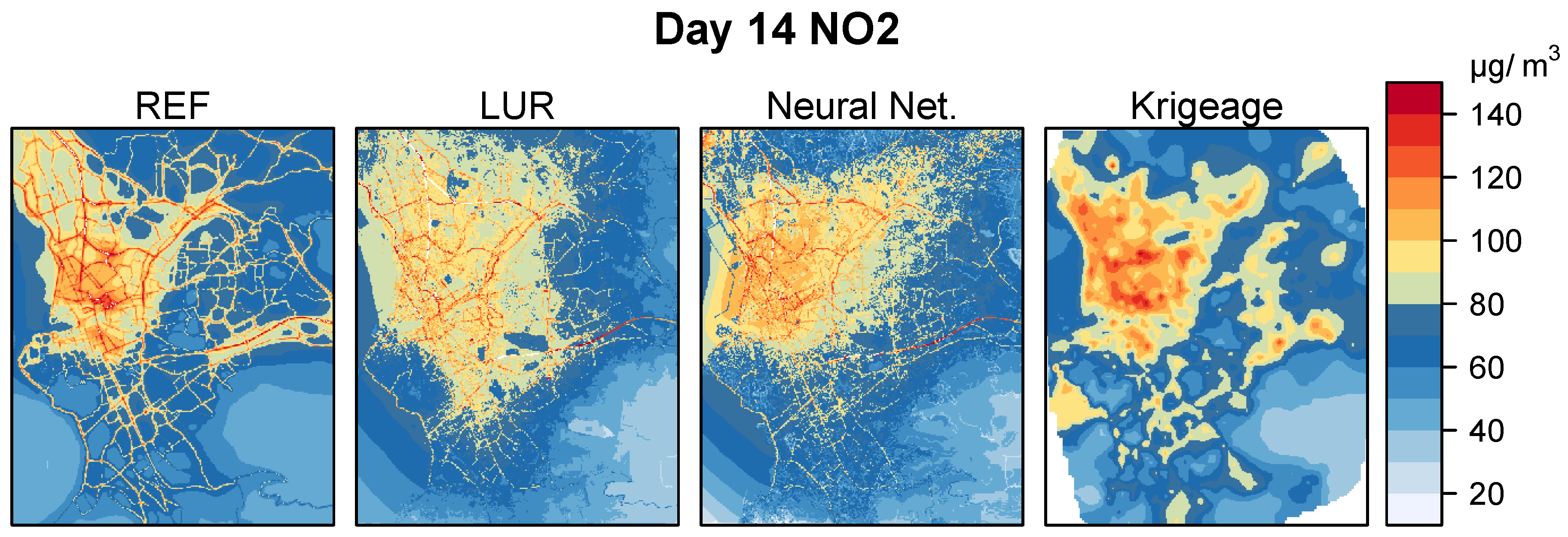
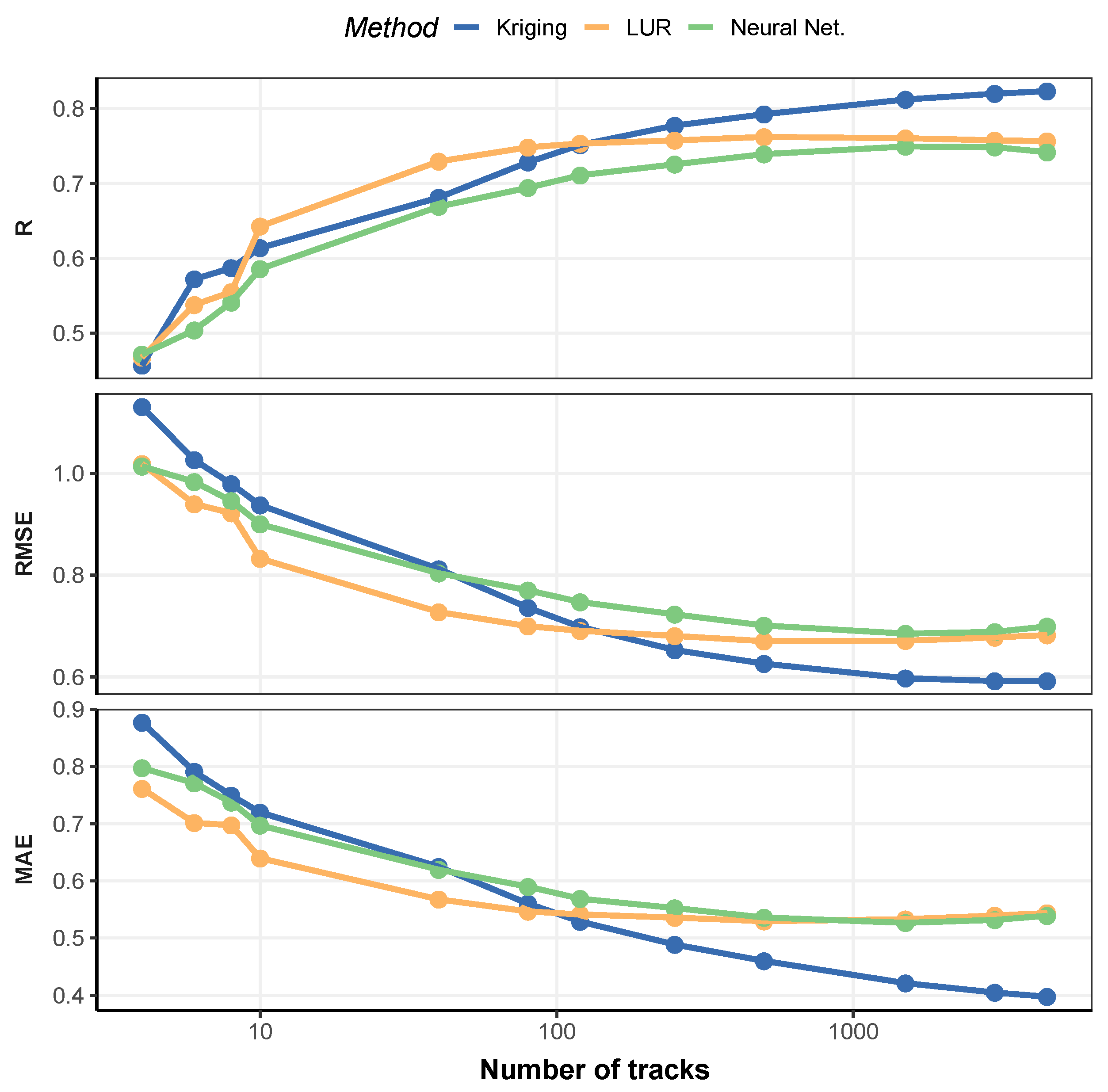
3.2. Model Prediction and Sensitivity
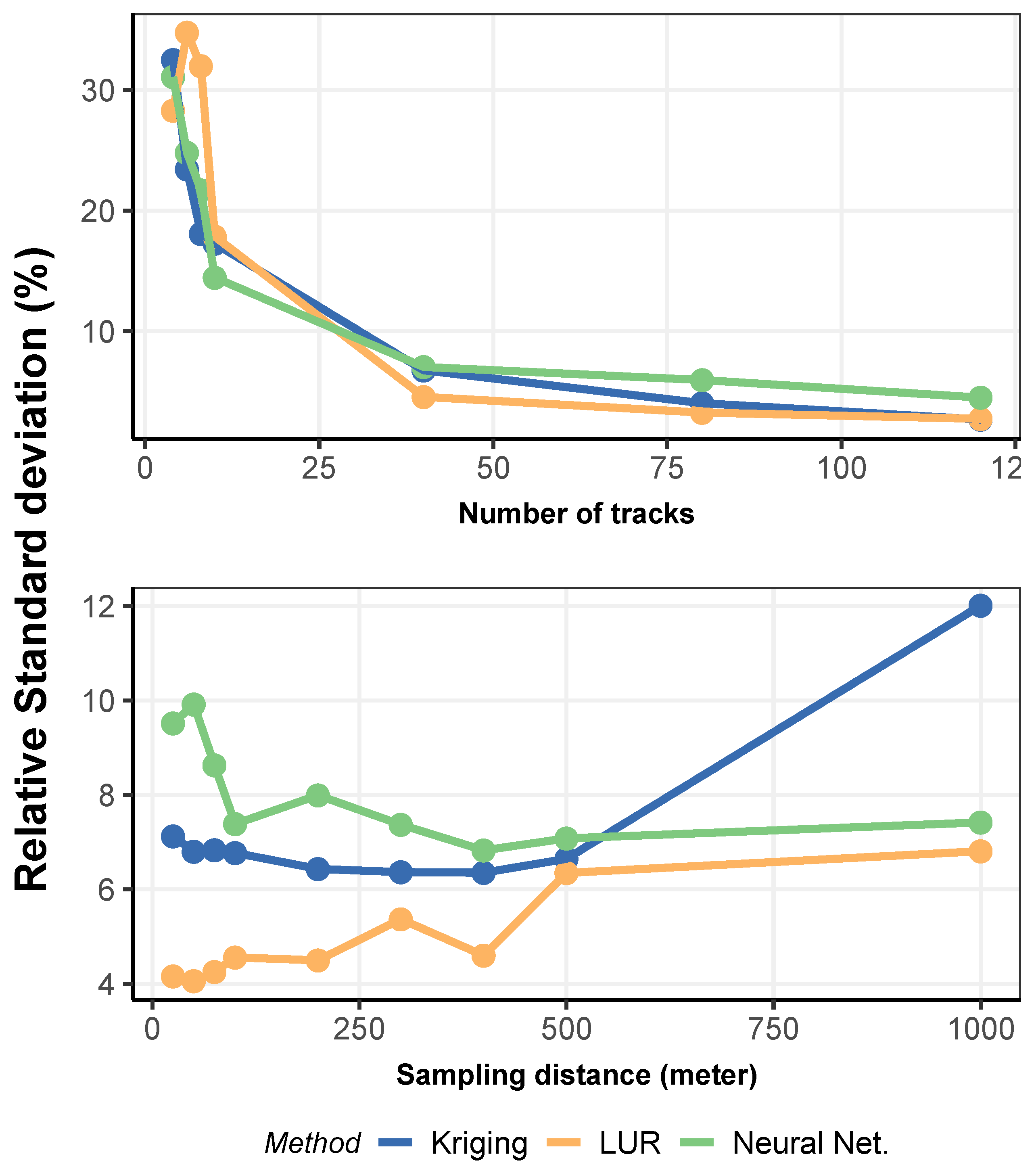
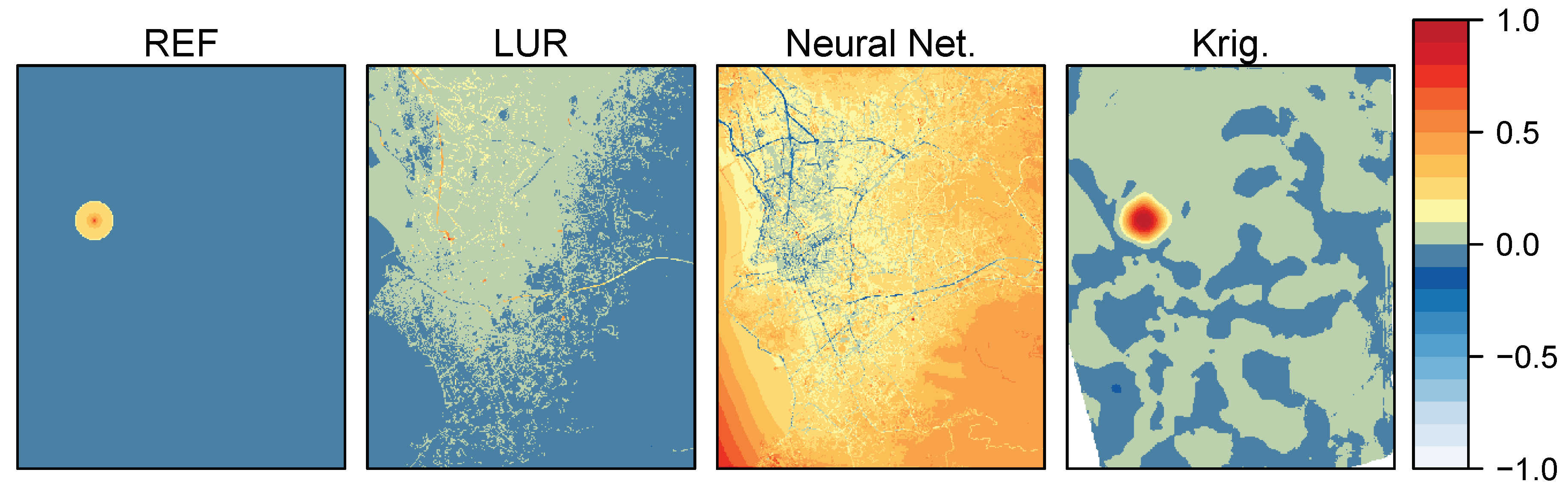
3.3. Sensitivity of the Methods to a Perturbation
4. Conclusions and Outlook
Author Contributions
Funding
Conflicts of Interest
References
- World Health Organization. Evolution of WHO Air Quality Guidelines Past, Present and Future; OCLC: 1075973767; World Health Organization: Geneva, Switzerland, 2017. [Google Scholar]
- Marjovi, A.; Arfire, A.; Martinoli, A. High Resolution Air Pollution Maps in Urban Environments Using Mobile Sensor Networks. In Proceedings of the International Conference on Distributed Computing in Sensor Systems, Fortaleza, Brazil, 10–12 June 2015. [Google Scholar] [CrossRef]
- Thunis, P.; Miranda, A.; Baldasano, J.M.; Blond, N.; Douros, J.; Graff, A.; Janssen, S.; Juda-Rezler, K.; Karvosenoja, N.; Maffeis, G.; et al. Overview of Current Regional and Local Scale Air Quality Modelling Practices: Assessment and Planning Tools in the EU. Environ. Sci. Policy 2016. [Google Scholar] [CrossRef]
- Benedetti, A.; Morcrette, J.J.; Boucher, O.; Dethof, A.; Engelen, R.J.; Fisher, M.; Flentje, H.; Huneeus, N.; Jones, L.; Kaiser, J.W.; et al. Aerosol Analysis and Forecast in the European Centre for Medium-Range Weather Forecasts Integrated Forecast System: 2. Data Assimilation. J. Geophys. Res. 2009. [Google Scholar] [CrossRef]
- Tilloy, A.; Mallet, V.; Poulet, D.; Pesin, C.; Brocheton, F. BLUE-Based NO 2 Data Assimilation at Urban Scale. J. Geophys. Res. Atmos. 2013. [Google Scholar] [CrossRef]
- Menut, L.; Bessagnet, B. What Can We Expect from Data Assimilation for Air Quality Forecast? Part I: Quantification with Academic Test Cases. J. Atmos. Ocean. Technol. 2019, 36, 269–279. [Google Scholar] [CrossRef]
- Gressent, A.; Malherbe, L.; Colette, A.; Rollin, H.; Scimia, R. Data Fusion for Air Quality Mapping Using Low-Cost Sensor Observations: Feasibility and Added-Value. Environ. Int. 2020, 143, 105965. [Google Scholar] [CrossRef]
- Deville Cavellin, L.; Weichenthal, S.; Tack, R.; Ragettli, M.S.; Smargiassi, A.; Hatzopoulou, M. Investigating the Use of Portable Air Pollution Sensors to Capture the Spatial Variability of Traffic-Related Air Pollution. Environ. Sci. Technol. 2016. [Google Scholar] [CrossRef]
- Adams, M.D.; Kanaroglou, P.S. Mapping real-time air pollution health risk for environmental management: Combining mobile and stationary air pollution monitoring with neural network models. J. Environ. Manag. 2016. [Google Scholar] [CrossRef]
- Hoek, G.; Beelen, R.; Hoogh, K.D.; Vienneau, D.; Gulliver, J.; Fischer, P.; Briggs, D. A review of land-use regression models to assess spatial variation of outdoor air pollution. Atmos. Environ. 2008. [Google Scholar] [CrossRef]
- Jerrett, M.; Arain, A.; Kanaroglou, P.; Beckerman, B.; Potoglou, D.; Sahsuvaroglu, T.; Morrison, J.; Giovis, C. A review and evaluation of intraurban air pollution exposure models. J. Expo. Anal. Environ. Epidemiol. 2004. [Google Scholar] [CrossRef]
- Janssen, S.; Dumont, G.; Fierens, F.; Mensink, C. Spatial interpolation of air pollution measurements using CORINE land cover data. Atmos. Environ. 2008. [Google Scholar] [CrossRef]
- Ionescu, A.; Candau, Y.; Mayer, E.; Colda, I. Analytical determination and classification of pollutant concentration fields using air pollution monitoring network data: Methodology and application in the Paris area, during episodes with peak nitrogen dioxide levels. Environ. Model. Softw. 2000. [Google Scholar] [CrossRef]
- Sivaraman, V.; Carrapetta, J.; Hu, K.; Luxan, B.G. HazeWatch: A participatory sensor system for monitoring air pollution in Sydney. In Proceedings of the 38th Annual IEEE Conference on Local Computer Networks-Workshops, Sydney, Australia, 21–24 October 2013. [Google Scholar] [CrossRef]
- Su, J.G.; Jerrett, M.; Beckerman, B.; Wilhelm, M.; Ghosh, J.K.; Ritz, B. Predicting traffic-related air pollution in Los Angeles using a distance decay regression selection strategy. Environ. Res. 2009. [Google Scholar] [CrossRef] [PubMed]
- Hasenfratz, D.; Saukh, O.; Walser, C.; Hueglin, C.; Fierz, M.; Arn, T.; Beutel, J.; Thiele, L. Deriving high-resolution urban air pollution maps using mobile sensor nodes. Pervasive Mob. Comput. 2015. [Google Scholar] [CrossRef]
- Ghassoun, Y.; Ruths, M.; Löwner, M.O.; Weber, S. Intra-urban variation of ultrafine particles as evaluated by process related land use and pollutant driven regression modelling. Sci. Total. Environ. 2015. [Google Scholar] [CrossRef] [PubMed]
- Mueller, M.D.; Hasenfratz, D.; Saukh, O.; Fierz, M.; Hueglin, C. Statistical modelling of particle number concentration in Zurich at high spatio-temporal resolution utilizing data from a mobile sensor network. Atmos. Environ. 2016. [Google Scholar] [CrossRef]
- Li, S.; Zhai, L.; Zou, B.; Sang, H.; Fang, X. A Generalized Additive Model Combining Principal Component Analysis for PM2.5 Concentration Estimation. ISPRS Int. J. Geo-Inf. 2017, 6, 248. [Google Scholar] [CrossRef]
- Mercer, L.D.; Szpiro, A.A.; Sheppard, L.; Lindstrom, J.; Adar, S.D.; Allen, R.W.; Avol, E.L.; Oron, A.P.; Larson, T.; Liu, L.J.S.; et al. Comparing universal kriging and land-use regression for predicting concentrations of gaseous oxides of nitrogen (NOx) for the Multi-Ethnic Study of Atherosclerosis and Air Pollution (MESA Air). Atmos. Environ. 2011. [Google Scholar] [CrossRef]
- Kurt, A.; Gulbagci, B.; Karaca, F.; Alagha, O. An online air pollution forecasting system using neural networks. Environ. Int. 2008. [Google Scholar] [CrossRef] [PubMed]
- Zheng, Y.; Yi, X.; Li, M.; Li, R.; Shan, Z.; Chang, E.; Li, T. Forecasting Fine-Grained Air Quality Based on Big Data. In Proceedings of the 21th SIGKDD Conference on Knowledge Discovery and Data Mining, Sydney, Australia, 10–13 August 2015. [Google Scholar] [CrossRef]
- Hsieh, H.P.; Lin, S.D.; Zheng, Y. Inferring Air Quality for Station Location Recommendation Based on Urban Big Data. In Proceedings of the 21th ACM SIGKDD International Conference on Knowledge Discovery and Data Mining, Sydney, Australia, 10–13 August 2015. [Google Scholar] [CrossRef]
- Niska, H.; Hiltunen, T.; Karppinen, A.; Ruuskanen, J.; Kolehmainen, M. Evolving the neural network model for forecasting air pollution time series. Eng. Appl. Artif. Intell. 2004. [Google Scholar] [CrossRef]
- Onkal-Engin, G.; Demir, I.; Hiz, H. Assessment of urban air quality in Istanbul using fuzzy synthetic evaluation. Atmos. Environ. 2004. [Google Scholar] [CrossRef]
- Dons, E.; Poppel, M.V.; Kochan, B.; Wets, G.; Panis, L.I. Modeling temporal and spatial variability of traffic-related air pollution: Hourly land use regression models for black carbon. Atmos. Environ. 2013. [Google Scholar] [CrossRef]
- Romanowicz, R.; Young, P.; Brown, P.; Diggle, P. A recursive estimation approach to the spatio-temporal analysis and modelling of air quality data. Environ. Model. Softw. 2006. [Google Scholar] [CrossRef]
- Qi Gan, W.; Koehoorn, M.; Davies, H.W.; Demers, P.A.; Tamburic, L.; Brauer, M. Long-Term Exposure to Traffic-Related Air Pollution and the Risk of Coronary Heart Disease Hospitalization and Mortality. Environ. Health Perspect. 2011. [Google Scholar] [CrossRef]
- Russo, A.; Raischel, F.; Lind, P.G. Air quality prediction using optimal neural networks with stochastic variables. Atmos. Environ. 2013. [Google Scholar] [CrossRef]
- Elen, B.; Peters, J.; Poppel, M.V.; Bleux, N.; Theunis, J.; Reggente, M.; Standaert, A. The Aeroflex: A Bicycle for Mobile Air Quality Measurements. Sensors 2013, 13, 221–240. [Google Scholar] [CrossRef] [PubMed]
- Beirle, S.; Boersma, K.F.; Platt, U.; Lawrence, M.G.; Wagner, T. Megacity Emissions and Lifetimes of Nitrogen Oxides Probed from Space. Science 2011, 333, 1737–1739. [Google Scholar] [CrossRef] [PubMed]
- Madhavi Latha, K.; Highwood, E.J. Studies on Particulate Matter (PM10) and Its Precursors over Urban Environment of Reading, UK. J. Quant. Spectrosc. Radiat. Transf. 2006, 101, 367–379. [Google Scholar] [CrossRef]
- Deligiorgi, D.; Philippopoulos, K. Spatial Interpolation Methodologies in Urban Air Pollution Modeling: Application for the Greater Area of Metropolitan Athens, Greece. Adv. Air Pollut. 2011. [Google Scholar] [CrossRef]
- Wong, D.W.; Yuan, L.; Perlin, S.A. Comparison of spatial interpolation methods for the estimation of air quality data. J. Expo. Sci. Environ. Epidemiol. 2004. [Google Scholar] [CrossRef]
- AIRES Méditerranée. Available online: http://www.aires-mediterranee.org/ (accessed on 21 September 2020).
- AtmoSud. Available online: https://www.atmosud.org/ (accessed on 21 September 2020).
- Riviere, E.; Bernard, J.; Hulin, A.; Virga, J.; Dugay, F.; Charles, M.A.; Cheminat, M.; Cortinovis, J.; Ducroz, F.; Laborie, A.; et al. Air Pollution Modeling and Exposure Assessment during Pregnancy in the French Longitudinal Study of Children (ELFE). Atmos. Environ. 2019, 205, 103–114. [Google Scholar] [CrossRef]
- Menut, L.; Bessagnet, B.; Khvorostyanov, D.; Beekmann, M.; Blond, N.; Colette, A.; Coll, I.; Curci, G.; Foret, G.; Hodzic, A.; et al. CHIMERE 2013: A Model for Regional Atmospheric Composition Modelling. Geosci. Model Dev. 2013. [Google Scholar] [CrossRef]
- Mailler, S.; Menut, L.; Khvorostyanov, D.; Valari, M.; Couvidat, F.; Siour, G.; Turquety, S.; Briant, R.; Tuccella, P.; Bessagnet, B.; et al. CHIMERE-2017: From Urban to Hemispheric Chemistry-Transport Modeling. Geosci. Model Dev. 2017, 10, 2397–2423. [Google Scholar] [CrossRef]
- Carruthers, D.J.; Holroyd, R.J.; Hunt, J.C.R.; Weng, W.S.; Robins, A.G.; Apsley, D.D.; Thompson, D.J.; Smith, F.B. UK-ADMS: A New Approach to Modelling Dispersion in the Earth’s Atmospheric Boundary Layer. J. Wind Eng. Ind. Aerodyn. 1994, 52, 139–153. [Google Scholar] [CrossRef]
- Carruthers, D.; Stidworthy, A.; Clarke, D.; Dicks, J. Urban Emission Inventory Optimisation Using Sensor Data, an Urban Air Quality Model and Inversion Techniques. Int. J. Environ. Pollut. 2019, 4, 15. [Google Scholar] [CrossRef]
- Hood, C.; MacKenzie, I.; Stocker, J.; Johnson, K.; Carruthers, D.; Vieno, M.; Doherty, R. Air Quality Simulations for London Using a Coupled Regional-to-Local Modelling System. Atmos. Chem. Phys. 2018, 18, 11221–11245. [Google Scholar] [CrossRef]
- Haklay, M.; Weber, P. OpenStreetMap: User-Generated Street Maps. IEEE Pervasive Comput. 2008, 7, 12–18. [Google Scholar] [CrossRef]
- GEOFABRIK. Available online: https://www.geofabrik.de/ (accessed on 21 September 2020).
- Arain, M.A.; Blair, R.; Finkelstein, N.; Brook, J.R.; Sahsuvaroglu, T.; Beckerman, B.; Zhang, L.; Jerrett, M. The Use of Wind Fields in a Land Use Regression Model to Predict Air Pollution Concentrations for Health Exposure Studies. Atmos. Environ. 2007, 41, 3453–3464. [Google Scholar] [CrossRef]
- Wilton, D.; Szpiro, A.; Gould, T.; Larson, T. Improving Spatial Concentration Estimates for Nitrogen Oxides Using a Hybrid Meteorological Dispersion/Land Use Regression Model in Los Angeles, CA and Seattle, WA. Sci. Total Environ. 2010, 408, 1120–1130. [Google Scholar] [CrossRef]
- BBBike. Available online: https://www.bbbike.org/ (accessed on 21 September 2020).
- Kim, S.Y.; Yi, S.J.; Eum, Y.S.; Choi, H.J.; Shin, H.; Ryou, H.G.; Kim, H. Ordinary Kriging Approach to Predicting Long-Term Particulate Matter Concentrations in Seven Major Korean Cities. Environ. Health Toxicol. 2014, 29. [Google Scholar] [CrossRef]
- Li, J.; Zhang, H.; Chao, C.Y.; Chien, C.H.; Wu, C.Y.; Luo, C.H.; Chen, L.J.; Biswas, P. Integrating Low-Cost Air Quality Sensor Networks with Fixed and Satellite Monitoring Systems to Study Ground-Level PM2.5. Atmos. Environ. 2020, 223, 117293. [Google Scholar] [CrossRef]
- Oliver, M.A.; Webster, R. Basic Steps in Geostatistics: The Variogram and Kriging; SpringerBriefs in Agriculture; Springer International Publishing: Cham, Switzerland, 2015. [Google Scholar] [CrossRef]
- Hiemstra, P.H.; Pebesma, E.J.; Twenhöfel, C.J.W.; Heuvelink, G.B.M. Real-time automatic interpolation of ambient gamma dose rates from the Dutch radioactivity monitoring network. Comput. Geosci. 2009. [Google Scholar] [CrossRef]
- Wood, S.N. Generalized Additive Models: An Introduction with R; Chapman & Hall: Boca Raton, FL, USA, 2017. [Google Scholar]
- Jain, A.K.; Mao, J.; Moidin Mohiuddin, K. Artificial Neural Networks: A Tutorial. Computer 1996. [Google Scholar] [CrossRef]
- Bergmeir, C.; Benítez, J.M. Neural Networks in R Using the Stuttgart Neural Network Simulator: RSNNS. J. Stat. Softw. 2012. [Google Scholar] [CrossRef]
- Kuhn, M. Building Predictive Models in R Using the caret Package. J. Stat. Softw. 2008. [Google Scholar] [CrossRef]
- Collectif Vélos En Ville. Available online: http://www.velosenville.org (accessed on 21 September 2020).


| Explanatory Variable | Description |
|---|---|
| Continuous features | |
| Position | Spatial coordinates |
| Altitude | Altitude above sea level (IGN base) |
| Distance to main roads | Distance to ’motorway’, ’trunk’ or ’primary’ roads in OSM calculated from roads layer |
| Buildings_a | Buildings density calculated from buildings_a layer |
| Maximum Speed | Speed limit extract from roads layer |
| Categorical features | |
| Network | Road and rail network merge of roads and railways layers |
| Transport | Transport infrastructure (bus stop, ferry terminal, taxi rank,...) |
| Landuse_a | Land use merged of de water_a, transport_a, traffic_a, natural_a and landuse_a |
| Traffic | Road network information (traffic lights, signaling, ...) |
| POIs | Points of interest of the city classified by main classes (points), merge of pois and pofw layers |
| POIs_a | Points of interest of the city classified by main classes (surface), merge of pois_a and pofw_a layers |
| Tree | Presence of one or more trees in the city calculated from natural layers |
| Designation | 2017 | 2018 | Simulated |
|---|---|---|---|
| Baille/Lodi | 294 | - | 764 |
| National/Guibal | 175 | - | 487 |
| Prado/Castellane | 639 | 727 | 1297 |
| Chave/Eugène Pierre | 88 | - | 332 |
| Joliette/République | 178 | - | 623 |
| Rome/Saint Louis | 388 | - | 214 |
| Vieux Port/Canebière | 522 | 667 | 965 |
| République/Sadi Carnot | 262 | - | 416 |
| Corniche/hélice | 157 | - | 819 |
| Michelet/vélodrome | 438 | 506 | 638 |
© 2020 by the authors. Licensee MDPI, Basel, Switzerland. This article is an open access article distributed under the terms and conditions of the Creative Commons Attribution (CC BY) license (http://creativecommons.org/licenses/by/4.0/).
Share and Cite
Bertero, C.; Léon, J.-F.; Trédan, G.; Roy, M.; Armengaud, A. Urban-Scale NO2 Prediction with Sensors Aboard Bicycles: A Comparison of Statistical Methods Using Synthetic Observations. Atmosphere 2020, 11, 1014. https://doi.org/10.3390/atmos11091014
Bertero C, Léon J-F, Trédan G, Roy M, Armengaud A. Urban-Scale NO2 Prediction with Sensors Aboard Bicycles: A Comparison of Statistical Methods Using Synthetic Observations. Atmosphere. 2020; 11(9):1014. https://doi.org/10.3390/atmos11091014
Chicago/Turabian StyleBertero, Christophe, Jean-François Léon, Gilles Trédan, Mathieu Roy, and Alexandre Armengaud. 2020. "Urban-Scale NO2 Prediction with Sensors Aboard Bicycles: A Comparison of Statistical Methods Using Synthetic Observations" Atmosphere 11, no. 9: 1014. https://doi.org/10.3390/atmos11091014
APA StyleBertero, C., Léon, J.-F., Trédan, G., Roy, M., & Armengaud, A. (2020). Urban-Scale NO2 Prediction with Sensors Aboard Bicycles: A Comparison of Statistical Methods Using Synthetic Observations. Atmosphere, 11(9), 1014. https://doi.org/10.3390/atmos11091014