Article

Impact of Physics Parameterizations on High-Resolution Air Quality Simulations over the Paris Region

1
INERIS, National Institute for Industrial Environment and Risks, Parc Technologique ALATA, 60550 Verneuil-en-Halatte, France
2
Sorbonne University, UPMC-Paris 06, DE129, 75005 Paris, France
*
Author to whom correspondence should be addressed.
Now at Citepa: Technical Reference Center for Air Pollution and Climate Change, 42, rue de Paradis, 75010 Paris, France.
Atmosphere 2020, 11(6), 618; https://doi.org/10.3390/atmos11060618
Submission received: 4 May 2020 / Revised: 1 June 2020 / Accepted: 4 June 2020 / Published: 11 June 2020
(This article belongs to the Special Issue Air Pollution and Environment in France)

Abstract

:
The accurate simulation of meteorological conditions, especially within the planetary boundary layer (PBL), is of major importance for air quality modeling. In the present work, we have used the Weather Research and Forecast (WRF) model coupled with the chemistry transport model (CTM) CHIMERE to understand the impact of physics parameterizations on air quality simulation during a short-term pollution episode on the Paris region. A lower first model layer with a 4 m surface layer could better reproduce the transport and diffusion of pollutants in a real urban environment. Three canopy models could better reproduce a 2 m temperature (T2) in the daytime but present a positive bias from 1 to 5 °C during the nighttime; the multi-urban canopy scheme “building effect parameterization” (BEP) underestimates the 10 m windspeed (W10) around 1.2 m s−1 for the whole episode, indicating the city cluster plays an important role in the diffusion rate in urban areas. For the simulation of pollutant concentrations, large differences were found between three canopy schemes, but with an overall overestimation during the pollution episode, especially for NO2 simulation, the average mean biases of NO2 prediction during the pollution episode were 40.9, 62.2, and 29.7 µg m−3 for the Bulk, urban canopy model (UCM), and BEP schemes, respectively. Meanwhile, the vertical profile of the diffusion coefficients and pollutants indicated an important impact of the canopy model on the vertical diffusion. The PBL scheme sensitivity tests displayed an underestimation of the height of the PBL when compared with observations issued from the Lidar. The YonSei University scheme YSU and Boulac PBL schemes improved the PBL prediction compared with the Mellor–Yamada–Janjic (MYJ) scheme. All the sensitivity tests, except the Boulac–BEP, could not fairly reproduce the PBL height during the pollution episode. The Boulac–BEP scheme had significantly better performances than the other schemes for the simulation of both the PBL height and pollutants, especially for the NO2 and PM2.5 (particulate matter 2.5 micrometers or less in diameter) simulations. The mean bias of the NO2, PM2.5, and PM10 (particulate matter 10 micrometers or less in diameter) prediction were −5.1, 1.2, and −8.6 µg m−3, respectively, indicating that both the canopy schemes and PBL schemes have a critical effect on air quality prediction in the urban region.

1. Introduction

Nowadays, around 55% of the world’s population lives in urban areas, and this number is expected to increase by 68% by 2050. The European Environment Agency annual report has pointed out around 25% of the European urban population are exposed to air quality exceeding the European Union air quality standards [1], and air pollution is the leading preventable risk factors for premature death in Europe, being responsible for 400,000 deaths per year directly or indirectly. In addition, built-up surfaces that are mainly composed of artificial buildings and cement pavement which are clearly distinguished from natural surfaces favor heat accumulation [2,3]. Recent research shows that in urban regions, Urban Heat Islands (UHIs) can be observed by a difference of about 1.5–2 °C compared to rural area temperatures, and about 2.0–2.5 °C difference can be observed over densely built-up areas [4]. The UHI has a negative effect on the planetary boundary layer (PBL) height [5] and surface wind speed, which affects the transport and dispersion of pollutants. Overall, the UHI changes the local atmospheric dynamic [6], significantly influences local air pollution, reduces visibility, increases water usage, and enhances heat-related morbidity [7,8]. In modeling studies, detailed information on urban parameters is critical for the simulation of the UHI effect. Studies conducted in Taiwan have found that the urban canopy model can improve the prediction of UHI intensity, boundary layer development, land–sea breeze [9], and precipitation [5]. Air pollution prediction is crucial in order to inform a large fraction of the population and take adequate short- and long-term measures to improve air quality. The use of air quality modelling tools at high resolution is now common but remains a challenge, because buildings create local modifications in air flows and modify surface energy budgets and roughness, leading to very complex processes which make air quality simulation particularly difficult in the near-ground layers [10,11,12,13]. Chemical transport models usually require numerical weather prediction (NWP) models, which provide meteorological input data [14,15]. High-resolution urban canopy parameters databases are becoming more and more available for cities [16,17]. NWP models with different physics parameterizations have been widely used in recent decades to simulate air quality over urban regions, especially the widely used community mesoscale Advanced Research Weather Research and Forecasting (ARW-WRF) model. Studies show that physics parameterizations play a critical role both in meteorological and air quality simulation or forecast [18,19,20,21,22]. For example, the Planetary Boundary Layer (PBL) height is determined by the heat and momentum exchanges between the PBL and the surface. In meteorological models, the PBL height is calculated by the PBL scheme. Therefore, the PBL scheme is a crucial factor in simulating the formation and evolution of air pollution [23,24,25]. Studies on different PBL parameterization schemes have shown that an accurate description of the meteorological conditions within the PBL via an appropriate parameterization scheme is important for air pollution modeling [26]. Some studies have presented the influences of meteorological models on pollutant concentrations; they estimate that uncertainties of PBL heights from the different models are one of the major sources of the differences in Particulate Matter (PM) concentrations [27,28]. Kleczeket et al. [29] compared three non-TKE (Turbulent Kinetic Energy) schemes and four TKE closures schemes; they found that non-TKE schemes tend to produce higher temperatures and wind speeds than in TKE schemes, especially during nighttime. Barlage et al. [13] also had a similar result between TKE and non-TKE schemes at night and found that PBL schemes have little effect on model performances in urban locations during daytime. Some other studies indicate that most PBL schemes slightly overestimate near-ground wind speed [30]; a possible reason could be the omission of the effect of unresolved topographic features on the momentum flux [31].
For the first time, the chemistry transport model CHIMERE model has been used with a very low first layer of about 4 m to simulate the air quality. In order to understand the impact of physics parameterizations and improve high-resolution air quality simulation, various WRF configurations have been tested over the Paris region during a critical pollution episode occurring from 27th November to 4th December 2016. In this study, we examine three different PBL schemes: (1) the Mellor–Yamada–Janjic scheme (MYJ), (2) the YonSei University scheme (YSU), and (3) the Bougeault and Lacarrere scheme (Boulac); and three canopy schemes, (1) a reference scheme (Bulk) which does not consider urban canopy parameters, (2) a single urban canopy model (UCM) which simply defines the urban geometry as two-dimensional street canyons but considers the three-dimensional nature of urban morphologies, and (3) a multilayer urban canopy model considering building effect parameterization (BEP). BEP was developed by Martilli et al. [32], and allows the direct interaction between buildings and low atmospheric layers and therefore is more realistic in reproducing urban effects [16]. This work will inform the air quality community on our ability to assess and understand the atmospheric transport of air pollutants over cities for operational forecast with air quality models.

2. Model Description and Experiment Design

2.1. WRF Model Description

Several studies [33,34,35] demonstrate the importance of physics parameterizations in driving air quality modelling outputs. As the first step of this work, the WRF model (Version 3.9.1) is used to simulate the meteorological conditions. The WRF model provides several options for the parameterizations (details can be found in the WRF user manual) of physical processes, including multiple longwave and shortwave radiation schemes, surface layer schemes, land surface schemes, urban canopy schemes, and boundary layer schemes. The initial and boundary conditions are issued from the Global Forecasting System (GFS) analysis data from the National Centers for Environmental Prediction (NCEP), available at a 0.25° × 0.25° resolution at six-hourly time steps. The spectral nudging in WRF simulation is a way to constrain large-scale circulation and constrain the model to be more consistent with observations [36]. However, strong nudging may filter out extreme episodes, since nudging pushes the model toward a relatively smooth state [37]. Therefore, a weak spectral nudging above PBL has been tested to improve the accuracy of the downscaled fields but not filter out the simulation of extreme episodes.
The experiment set includes 11 simulations, which are conducted for a winter period from 27th November to 4th December 2016 and are designed to test the sensitivity of the surface meteorological variables and pollutant concentrations at these different physics parametrizations. Table 1 summarizes the parametrizations which are tested in the study.
The UCM is a single urban canopy layer model used to consider the effects of urban geometry on the surface energy balance and wind shear for urban regions [38,39]. This model includes shadows from buildings; canyon orientation; the diurnal variation in the azimuth angle; the reflection of short and long wave radiation; wind profiles in the canopy layer; anthropogenic heating associated with energy consumption by human activities; and multi-layer heat transfer equations for roof, wall, and road surfaces. The BEP is the multilayer canopy layer scheme. This scheme considers the sub-grid wall, roof, and road effects on radiation and fluxes but does not include the energy exchange between the inside and outside of buildings.
The MYJ PBL scheme uses the 1.5-order turbulence closure model of Mellor and Yamada [40] to represent turbulence above the surface layer [41,42]. The MYJ scheme determines eddy viscosity K-coefficients from prognostically calculated turbulent kinetic energy. The YSU PBL scheme is a first-order non-local scheme that uses a parabolic K-profile in an unstable mixed layer with the addition of an explicit term to treat the entrainment layer at the top of the PBL [28]. Hong et al. [43] enhanced mixing in the stable boundary layer by increasing the critical Bulk Richardson number from zero to 0.25. The Boulac PBL scheme was developed by Bougeault and Lacarrère [44] and is also a TKE prediction scheme and designed to work with a multi-layer urban model.

2.2. CHIMERE Model Description

The chemistry transport model (CTM) CHIMERE (Version 2013) [45] is used for air quality modeling in the present study. CHIMERE is a state-of-the-art Eulerian offline CTM model; it requires pre-calculated boundary conditions, emission fluxes, and meteorological variables. For the studied period, 27th November to 4th December 2016, an 8-day spin-up period is performed for initialization issues. The vertical turbulent mixing in CHIMERE takes place only within the boundary layer, which is calculated by meteorological parameters such as surface temperature and the wind speed issued from the WRF simulation. The first CHIMERE layer is set to 4 m. The vertical dispersion in CHIMERE is mostly controlled by the PBL height and a turbulent flux modeled by a vertical eddy diffusion coefficient (Kz). The horizontal diffusion is neglected in CHIMERE. The PBL height is directly taken from the WRF output and capped at a minimal value of 20 m to avoid unrealistic simulations. In CHIMERE, the Kz is calculated using the parameterization of Troen and Mahrt [46] in Equation (1):
K z = k w s z ( 1 z h ) 2 ,
where k is the von Karman constant set to 0.41, z is the altitude, h is the boundary layer height, and ws is the vertical scale given by the similarity formulae.
The emissions of pollutants include several different gaseous and aerosol species. Those emissions can be split into four parts: anthropogenic emissions, biogenetic emissions, mineral dust emissions, and fire emissions. The anthropogenic emissions play a critical role in the CTM model, since they include all human activities, especially in megacities, and they are the only source we can reduce. For Europe region studies, anthropogenic emissions of gases and PM are generated with the Netherlands Organization for Applied Scientific Research (TNO) emission inventory [47], which is updated every six months. Biogenic emissions are estimated with the Model of Emissions and Gases and Aerosols from Nature (MEGAN). Mineral dust emissions are parameterized by Menut et al. [48]. The resolution TNO emission inventory is 0.125° × 0.0625° longitude–latitude or approximately 7 × 7 km, and the spatial resolutions of the emission data are recomputed from the TNO emission inventory for each domain. Driven by those input data, CHIMERE provides the hourly concentrations of tens of species at a regional scale; detailed descriptions of the model can be found in several previous studies [43,47,48,49,50]. The aerosol module accounts for both inorganic and organic species, such as sulfate, nitrate, ammonium, primary organic matter, element carbon, secondary organic aerosol, sea salt, dust, and water. The aerosol size is assuming discrete aerosol size sections and that the particles are internally mixed. Nine diameter bins, from 10 nm to 10 μm, with 5 bins below 1 μm, are used [51].

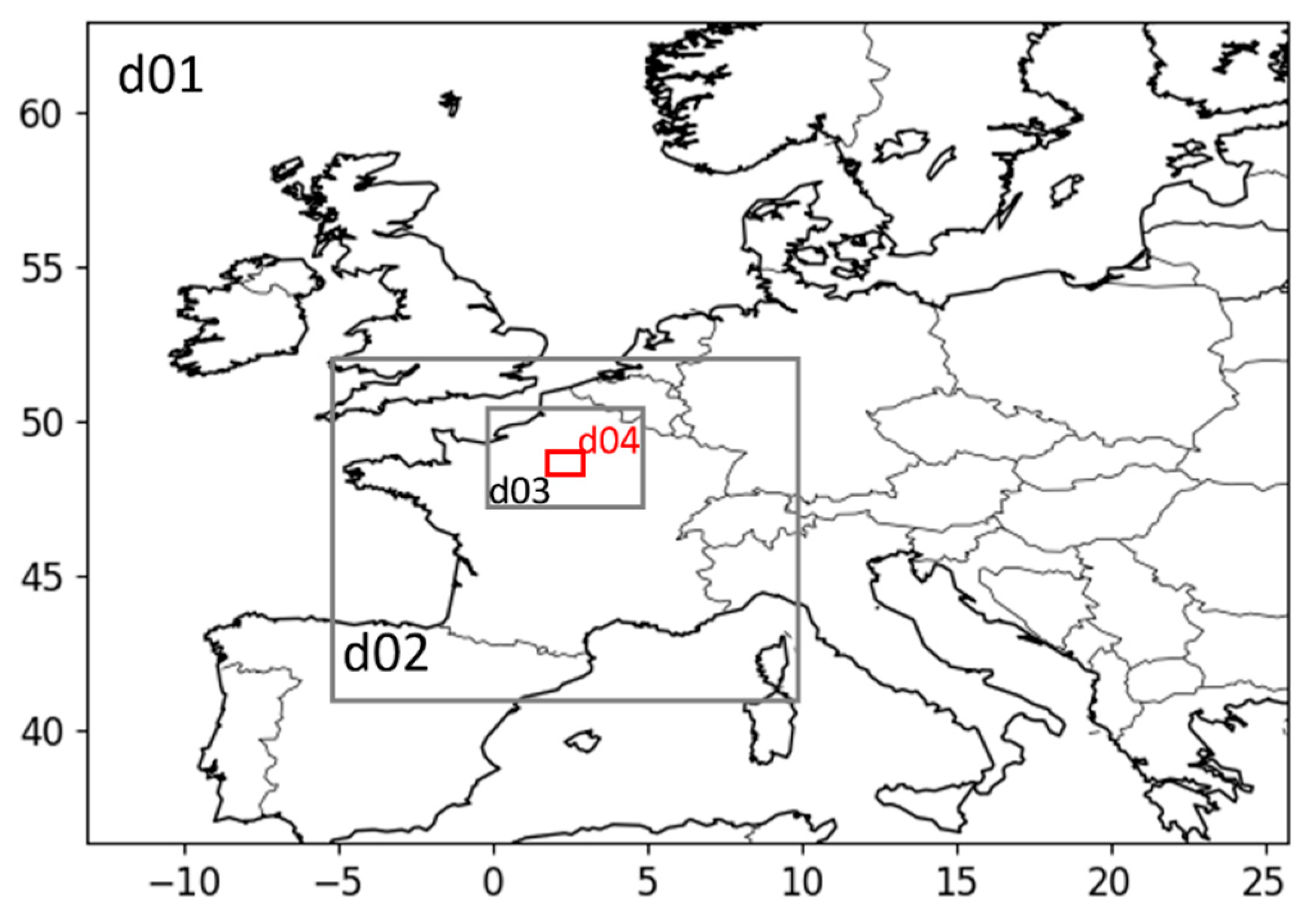
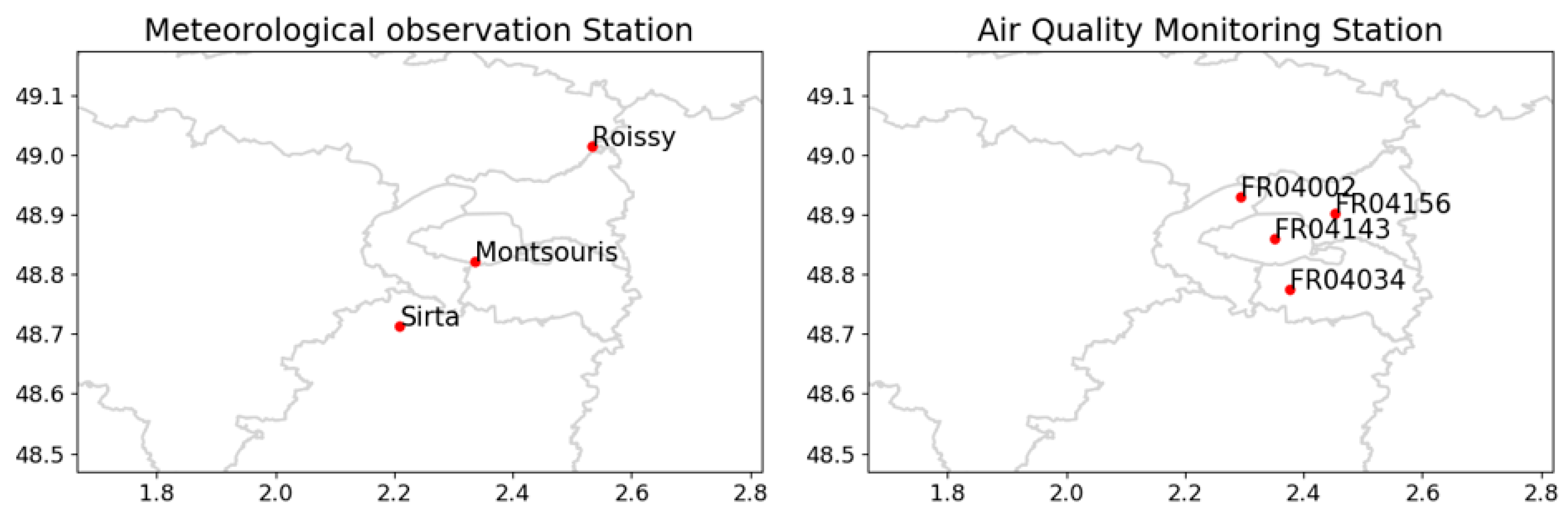
2.3. Domains Setup and Observations Data

In order to calculate realistic meteorological input variables and pollutant concentrations, the system is configured with four nested-grid domains (Figure 1) over Europe, France, the north of France, and Ile-de-France, with cell sizes of 45 (d01), 15 (d03), 5 (d02), and 1.67 km (d04), respectively. The finest grid domain (d04) used has 83 × 77 grid points and covers the whole Ile-de-France region, including urban, sub-urban, and rural areas. The WRF simulation is discretized vertically on 52 vertical levels from the surface to the top (50hPa), with 20 levels below 1000 m and the lowest level at 2 m, the complete name list of the WRF simulation can be found in List.S1. In order to take full advantage of the physical parameterizations, the CHIMERE simulation is performed with the same horizontal domains as the WRF; the 52 vertical levels from the WRF simulation are projected onto 33 levels in CHIMERE. The ground layer of the CHIMERE domains is at 999.5 hPa from about 4 m up to over 5000 m, with 15 levels below 1000 m. Such a low ground level could effectively reproduce the transport and diffusion of pollutants in a real urban environment.
Two types of observation data are used in the present study: (i) three meteorological observation stations operated by METEO FRANCE and SIRTA were used to evaluate the simulated surface meteorological variables from the model; and (ii) the hourly surface concentrations of criteria pollutants (NO2, PM2.5, and PM10) issued from AIRPARIF, the official Paris air quality network. The location of the three meteorological observation stations (Montsouris, Roissy, Sirta) and the four air quality monitoring stations can be found in Figure 2; they are urban or sub-urban background stations. The FR04143 air quality monitoring station is located in the city center. “Roissy” is a synoptic station of the Paris international Airport; “Montsouris” is an historical meteorological station located within Paris, operating since 1869; “Sirta” is a recent station located in a suburban environment.

3. Results and Discussions

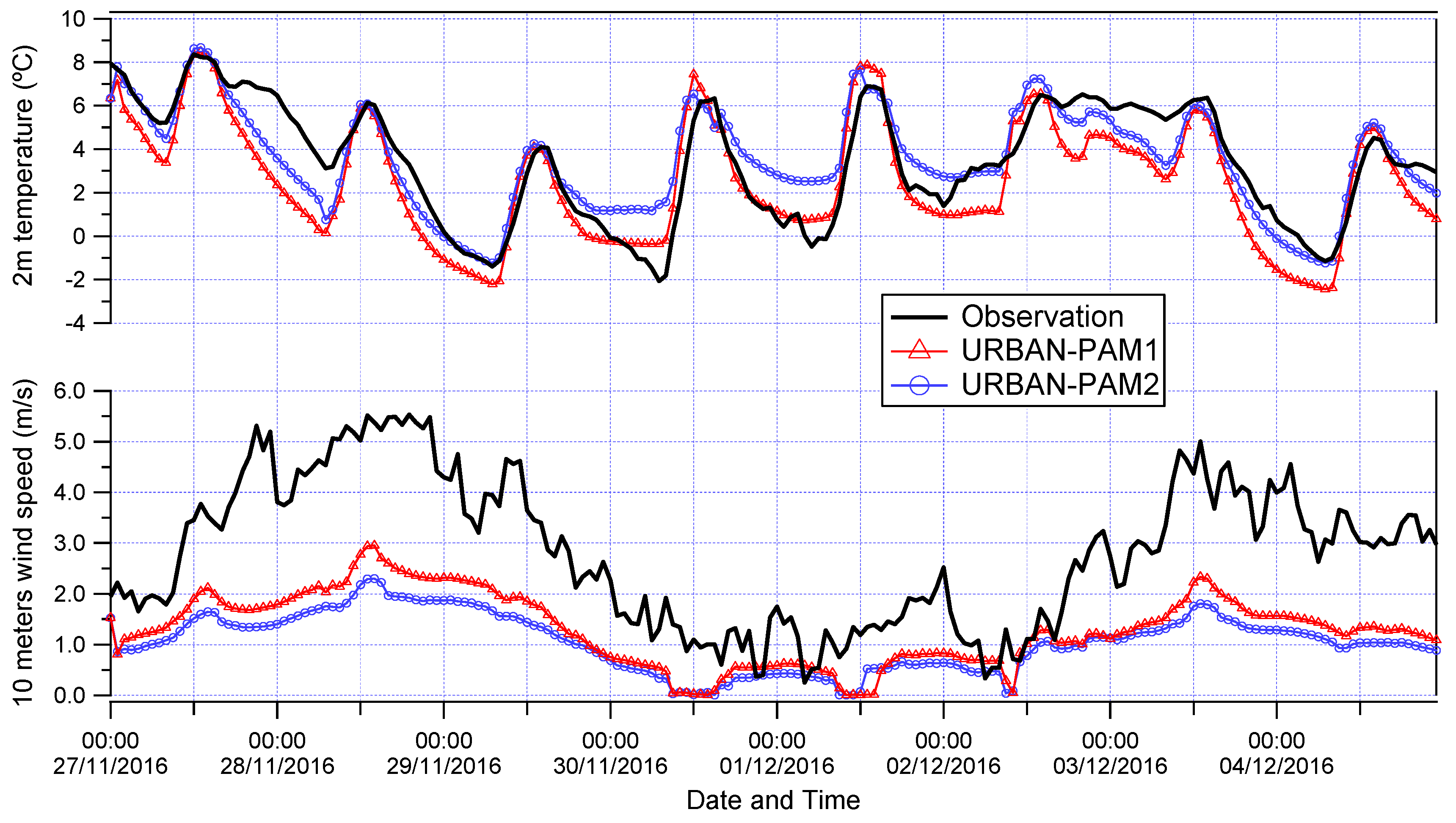
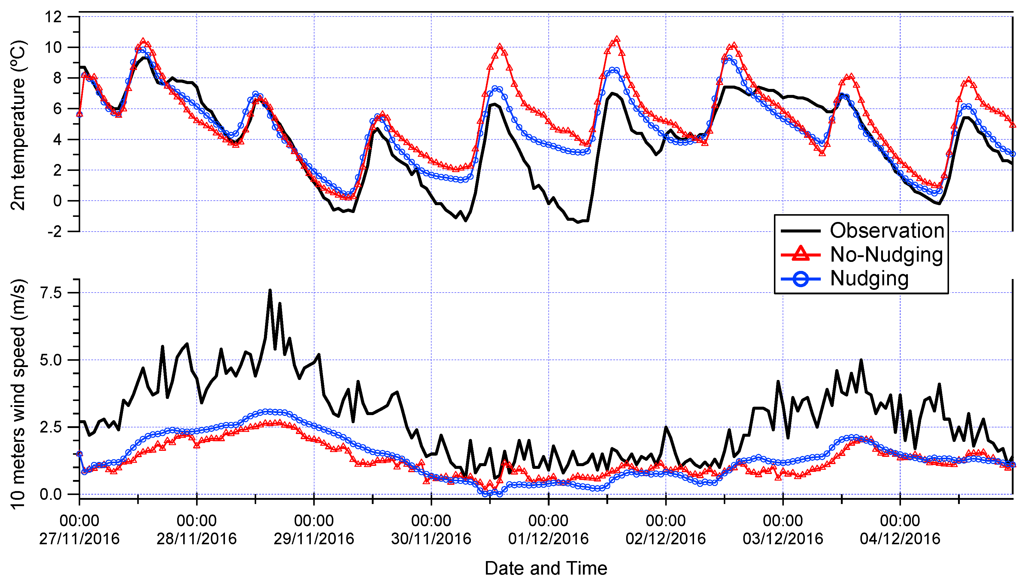
3.1. Urban Parameters and Nudging Tests

The urban canopy model in the WRF simulation affects the modeling of several important meteorological variables for air quality issues (e.g., 10 m wind speed W10, 2 m surface temperature T2, and PBL height). It changes the vertical distribution of atmospheric pollutants by modifying the boundary layer height and mixing. Geometric and thermal parameters, including anthropogenic heat, thermal conductivities, and heat capacity, have a significant effect on the transfer of momentum between the atmosphere and urban surface [52]. However, the representativeness of these parameters aggregated over a CTM grid cell remains highly uncertain, especially with a limited number of urban land-use types. The urban parameters (Table S1) used here are based on a previous study in Paris region [53,54] and default urban parameterization (URBPARM). The TBL tables in the WRF code are defined as URBAN-PAM1 and URBAN-PAM2, respectively. The RRTMG shortwave and longwave radiation scheme, MO similarity surface layer scheme, Noah land surface model, BEP urban canopy model, and MYJ boundary layer scheme are used for all simulations in this section. Figure 3 presents the time series of hourly-averaged T2 and W10 at Sirta station. The results show that simply modifying the values of the parameters has a strong impact on the outputs. The T2 presents a more positive correlation (0.86 than 0.81) in URBAN-PAM1 than in URBAN-PAM2, while the W10 has a more negative bias (−1.51 m than −1.42 m s−1) in URBAN-PAM1 than in URBAN-PAM2. A weak spectral nudging above the boundary layer for all the domains is also tested in this part. Figure 4 indicates that the spectral nudging technique is effective in improving the model skills. The performance benefits in Paris from the assimilation of meteorological data at Roissy airport in the global meteorological fields. Thus, URBAN-PAM1 and spectral nudging are used for all our sensitivity tests, which are discussed in the following sections.

3.2. Impact of the Urban Canopy Model

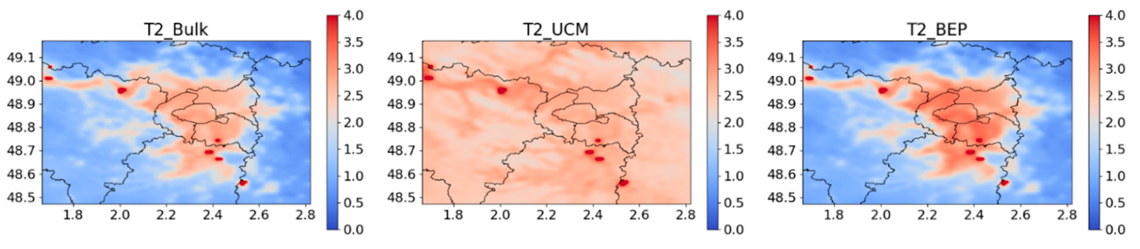
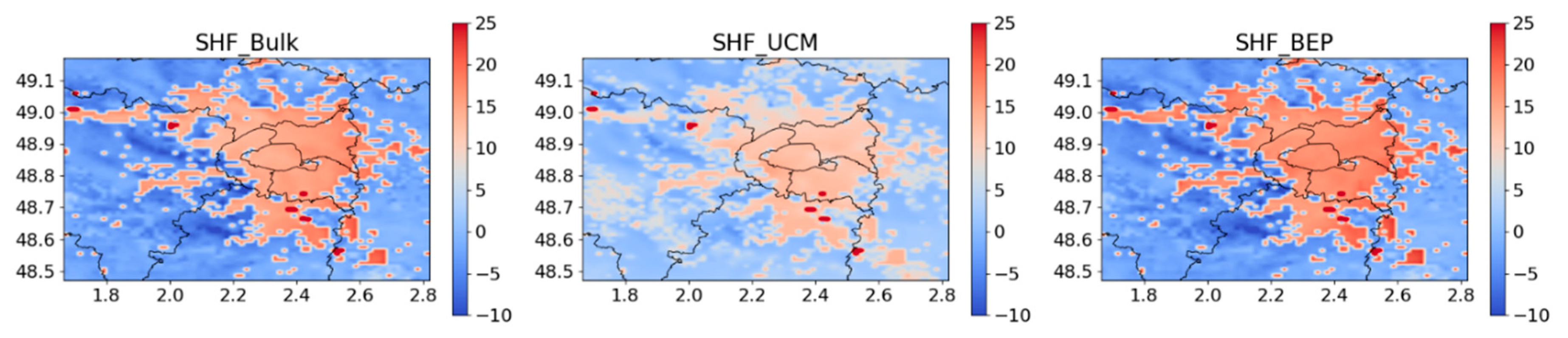
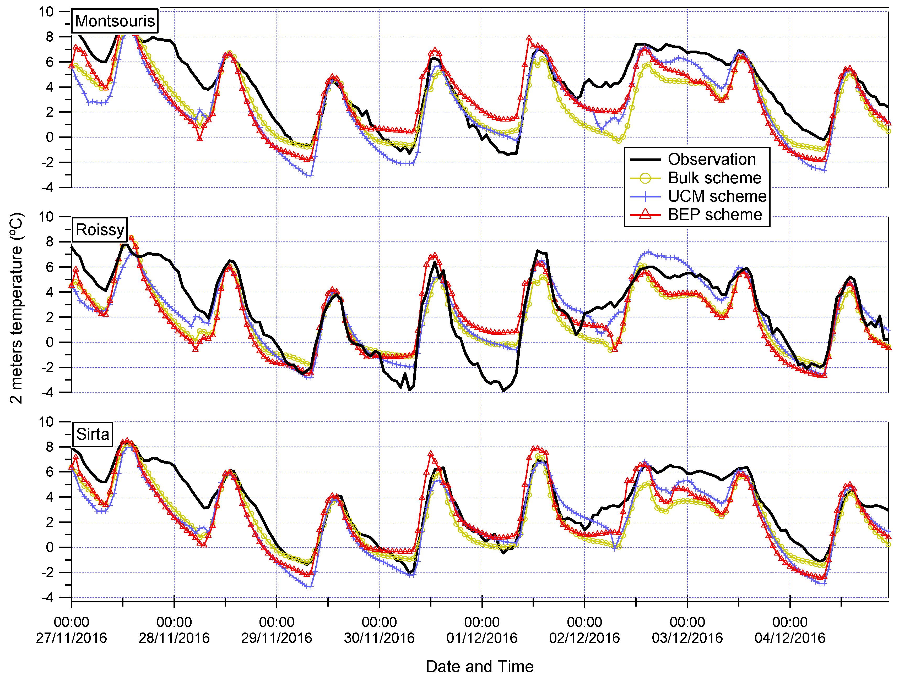
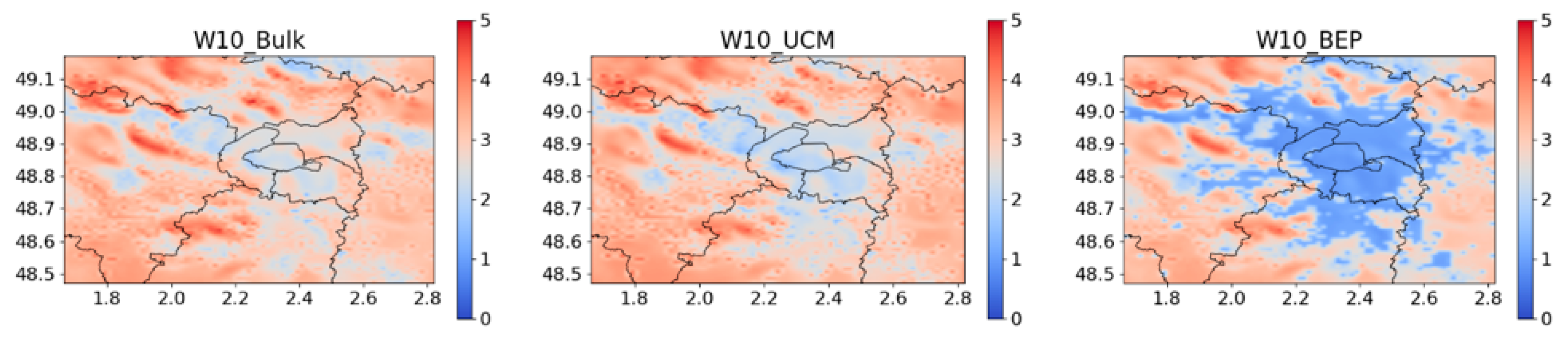
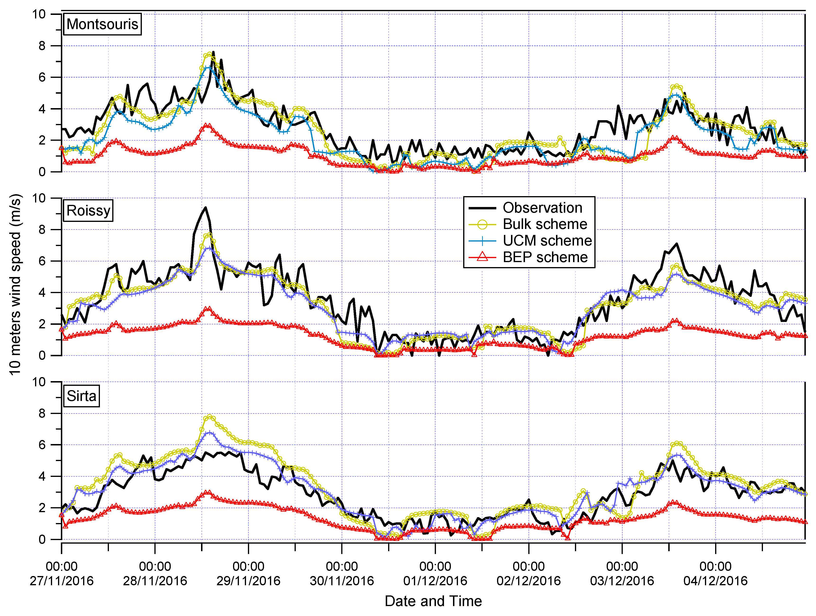
3.2.1. Ground Meteorological Variables

The RRTMG shortwave and longwave radiation schemes, the MO similarity surface layer scheme, and the Noah land surface model are used for all the simulations in this section. The whole period (27th November to 4th December 2016) is divided into two periods: a Particulate matter Episode (PE) from 30th November to 2nd December; and other days than the PE, which are defined as regular days (RD). No rainfall occurred over both then PE and the RD. Figure 5 presents the maps of averaged T2 simulated based on the Bulk, UCM, and BEP schemes in this period. All the schemes show a higher T2 in the urban region than the rural, and the BEP scheme displays the strongest UHI effect in the urban region, which gives a positive bias of up to 1 °C compared to the other two schemes. The Bulk and BEP schemes perform similarly in rural areas and display a negative bias (1–3 °C by Bulk and 1–4 °C by BEP) compared with urban areas, but the UCM scheme gives the highest T2 in rural areas, displaying a negative bias of about 0.5–1 °C compared with urban regions. A possible reason could be the overestimation of surface heat flux (SHF) in the rural areas. Figure 6 presents the averaged SHF in this period. The Bulk and BEP schemes display obvious differences between urban and rural regions, with a negative bias (around −25 to −35 W m−2) in rural compared to urban areas. The UCM scheme just produces a negative bias of −10 and −15 W m−2, respectively, in rural and urban areas, which could give an explanation of the overestimation of T2 in rural areas.
Results at the three meteorological stations are compared with the observations to evaluate the canopy scheme’s performance. Figure 7 presents the time series of hourly-averaged T2 during the whole period. The observed T2 varies between −1.4 and 9.3 °C, −3.9 and 7.8 °C, and −2.1 to 8.4 °C, with an average of 4.0, 2.6, and 4.9 °C at Montsouris, Roissy, and Sirta stations, respectively. Compared with the observations, all three schemes tended to underestimate the T2 during the period 16:00 p.m.–10:00 a.m. UTC on the 27th and 28th for all stations, while higher positive values were observed around midnight of the 1st December for Montsouris and Roissy stations, especially at Roissy, with a positive bias from 1.8 to 4.9 °C during the PE. The BEP scheme simulates relatively higher T2 at PE for all the stations because the BEP scheme simulates a stronger UHI than the other two schemes. All the schemes have the best performance at the Sirta site. Compared with the observations from three stations, the differences in the modelled T2 are minimal between three stations during the PE. However, there are significant differences in the observed T2 between the stations. For example, the minimum observed T2 are −1.4, −3.9, and −0.3 °C during the midnight of 1st December at Montsouris, Roissy, and Sirta stations, respectively. A possible reason could be the use of a single urban category in our WRF simulations, but in the real environment Montsouris and Sirta stations are closer to commercial and residential areas and Roissy is a synoptic station close to the airport, which could be assimilated as a rural environment with a weaker UHI effect, especially during nighttime.
Figure 8 shows the maps of the averaged W10 simulated for the Bulk, UCM, and BEP schemes in this period. All the schemes give a higher surface wind speed in rural areas than in urban regions; the Bulk scheme shows the weakest gradient from urban to rural areas, with a negative bias for 0.51 m s−1; UCM gives a relative higher negative bias than Bulk from 1 to 2 m s−1; and the BEP scheme had an obviously strongest impact from cities, displaying a negative bias around 3.5 m s−1. The comparison between the observations and models for W10 are displayed in Figure 9. The observed W10 varied between 0.6 m and 7.6 m s−1, 0.1 m and 9.4 m s−1, and 0.2 m and 5.5 m s−1, with an average of 2.3 m, 1.5 m, and 2.8 m s−1 in three meteorological observation stations (Montsouris, Roissy, Sirta), respectively. Both the observed and modelled W10 display much lower values during the PE than the RD. In contrast with the T2, the W10 does not display remarkable differences between stations. The BEP scheme tends to produce the lowest W10 throughout the whole period for all the stations. Bulk and UCM performed well for both the PE and RD. A possible reason could be due to the roughness length, which is not directly dependent on urban morphology for the UCM scheme, while the momentum sinks and drag force estimated by the BEP scheme depend on urban morphology in this study. Low wind speed leads to weak natural circulation and the accumulation of heat in the lower urban boundary layer, which in turn enhances the warming of the urban area [55]. This would explain why BEP has a relative higher T2 simulation than the other schemes during the PE. This sensitivity test indicates that more realistic urban morphologies are needed to improve the model performance, because the parameters used in the urban canopy scheme (e.g., albedo, heat capacity, and roughness length) strongly influence the surface energy balance and heat absorption.

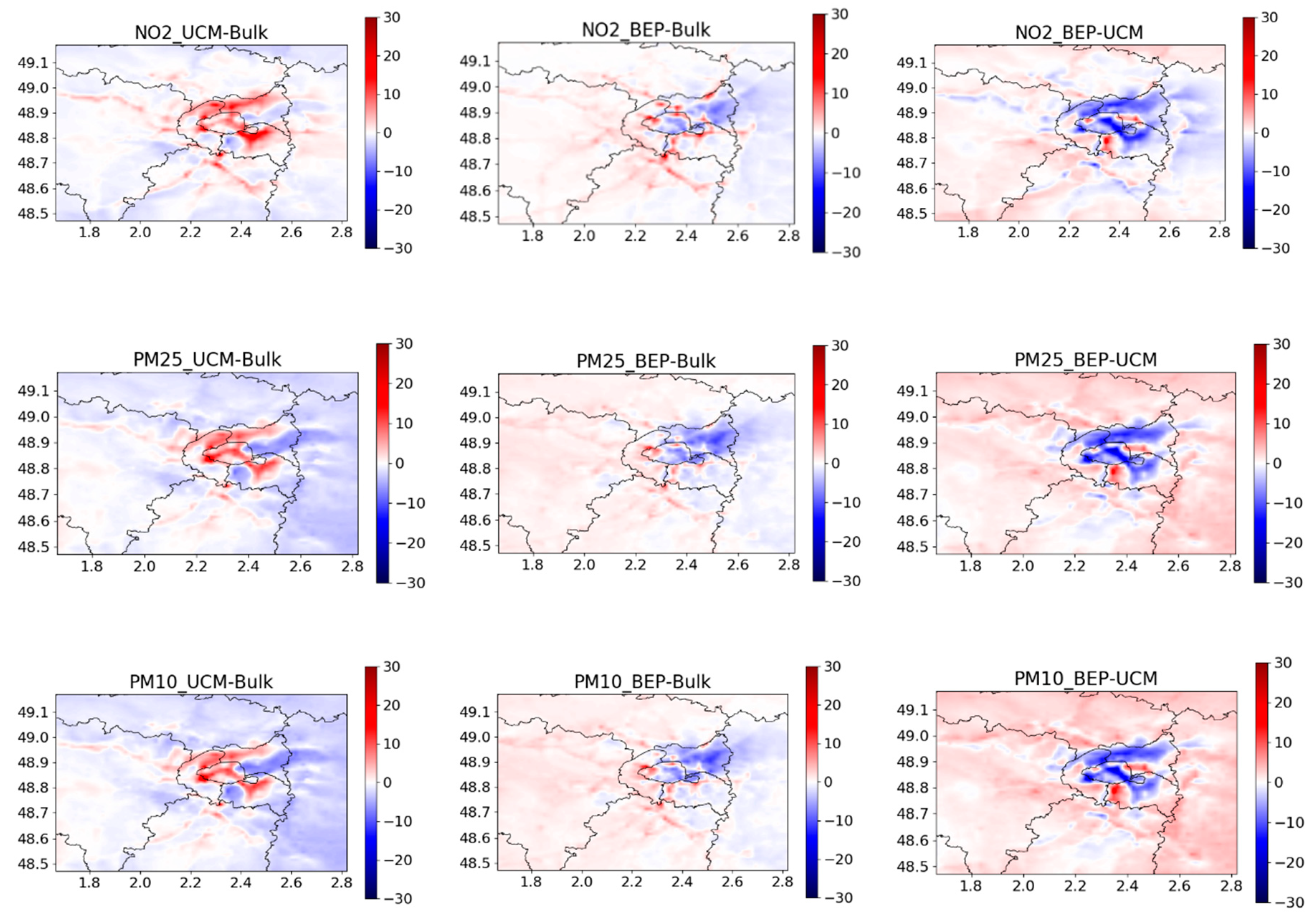
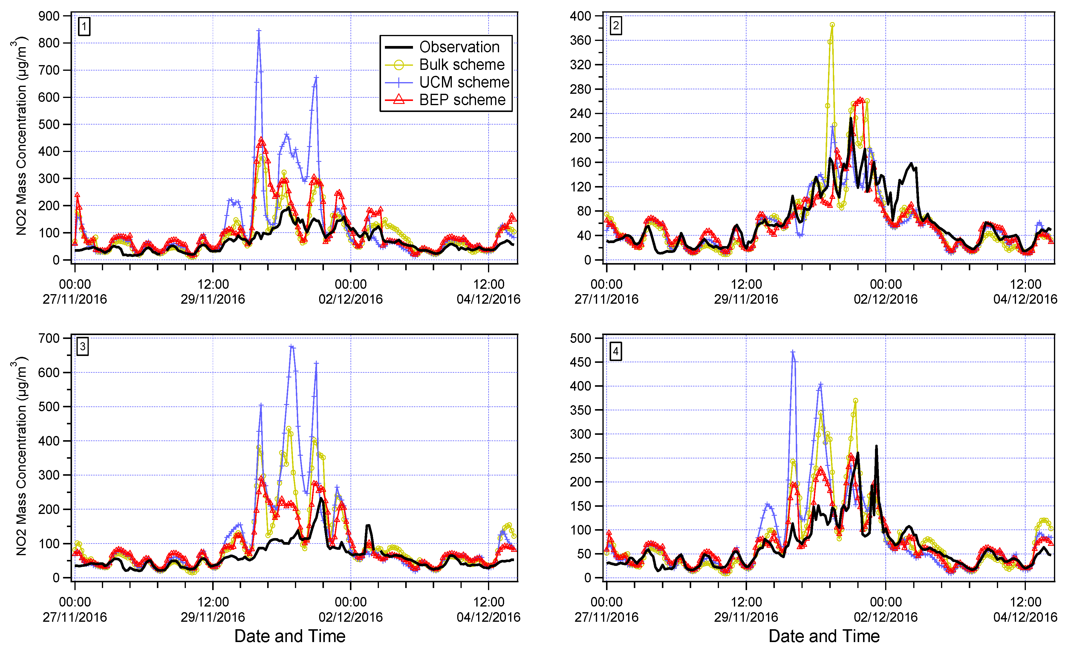
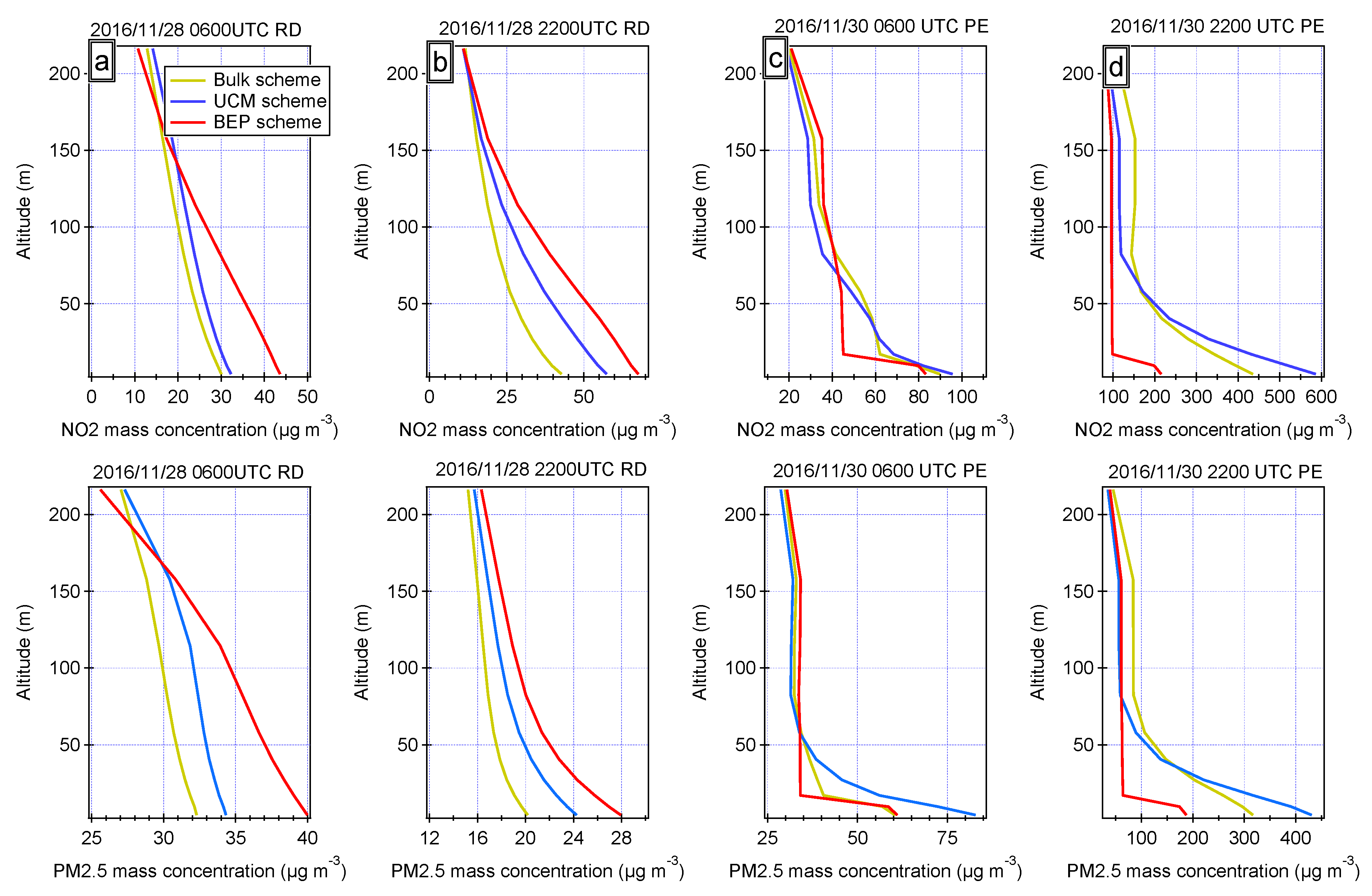
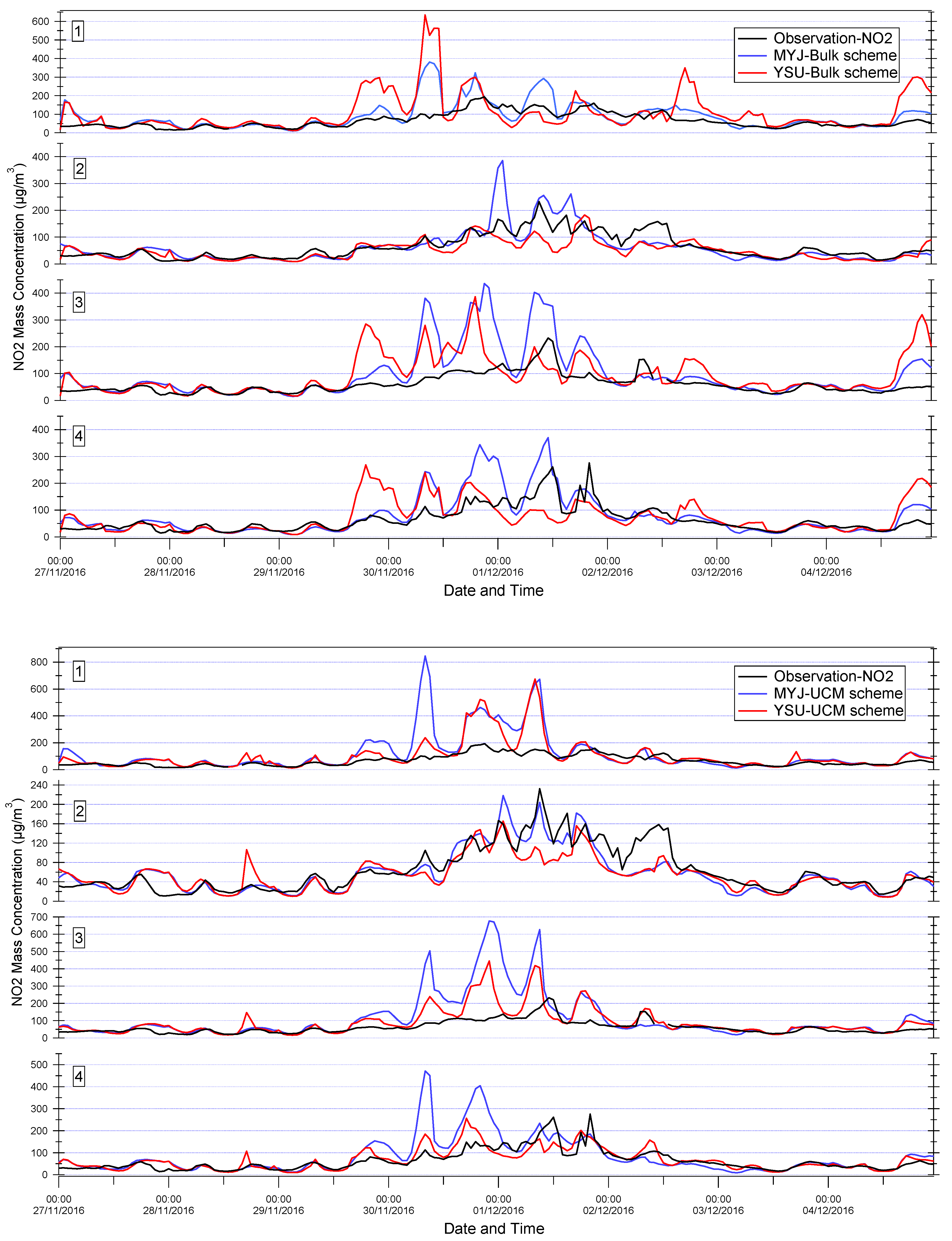
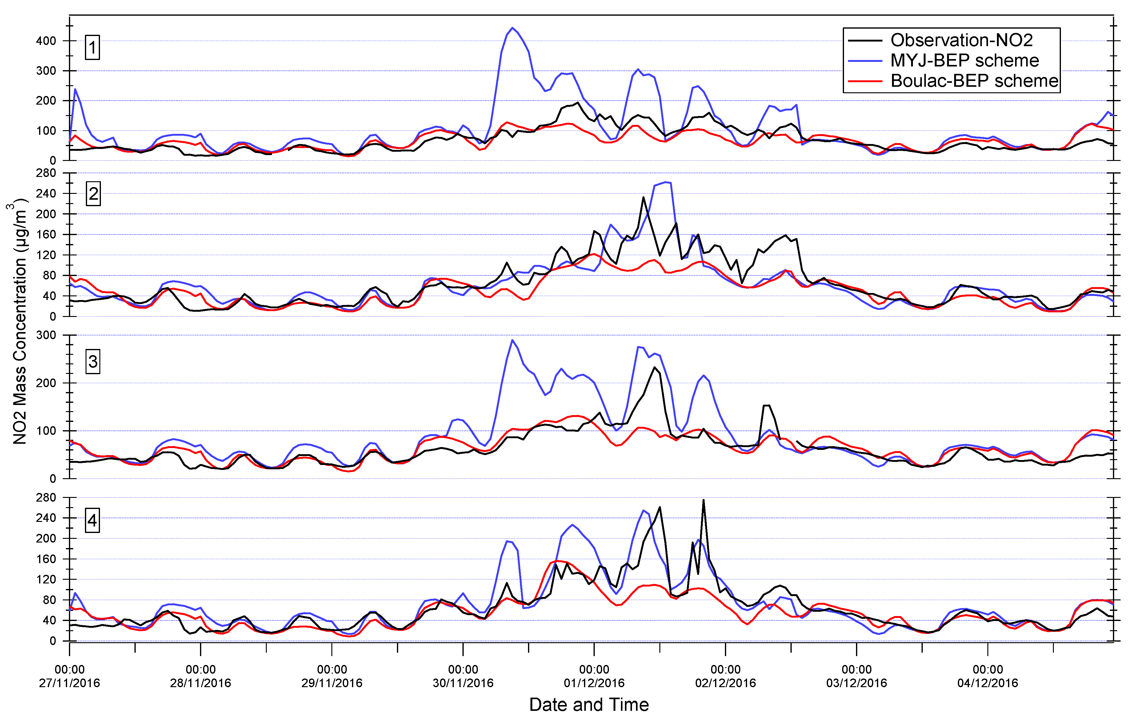
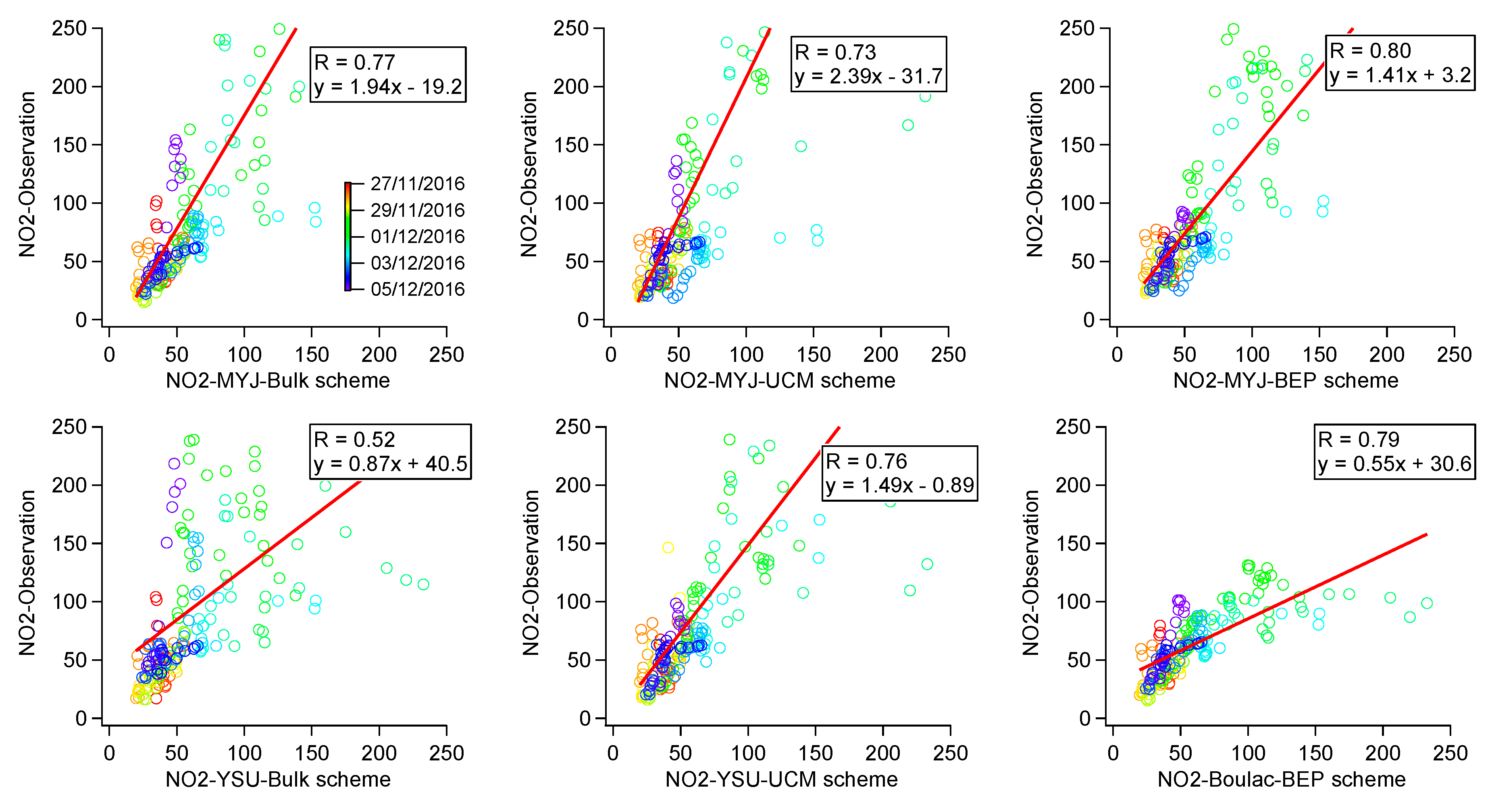
3.2.2. Air Quality Modeling

In this study, NO2, PM2.5, and PM10 concentrations are used to evaluate the impact of physics parameterizations on air quality simulations. NO2, which comes mainly from automobile exhaust emissions in cities, is selected to be an indicator of local pollution. Comparing the evolution and spatial patterns of NO2 versus the PM2.5 and PM10 gives an indication of the local contribution during this episode. Figure 10 presents the differences in pollutants distribution between each canopy scheme. The results show that, compared to the Bulk scheme, the pollutant concentrations from the BEP scheme were lower in the city center, but displayed an opposite behavior compared to the UCM scheme. The UCM scheme displayed higher pollutant concentrations in the urban area and lower pollutant concentrations in rural areas. Figure 11 presents the time series of NO2 mass concentrations for all the experiments compared to the observations for the four stations (the time series of PM2.5 and PM10 mass concentrations can be found in Figure S1). The average biases of the four stations is given in Table 2, and the time series of the biases are displayed in Figure S2. The results show that the BEP scheme gives the best performance for almost the whole period, especially during the PE. All the schemes can effectively predict air pollution during the RD, but they usually overestimate pollutant concentrations for all the stations during the PE; all the schemes had their worst performance in NO2 prediction, which means that the canopy schemes do not simulate well the emission of local air pollution. Figure 12 gives the vertical diffusion coefficient at daytime and nighttime in the RD and PE. The Bulk scheme has the highest vertical diffusion rate among the three schemes during the RD. Figure 13 presents the vertical profile of the NO2 and PM2.5 mass concentrations under 200 m; both NO2 and PM2.5 show the lowest vertical mass concentrations at low layers by the Bulk scheme and the highest vertical mass concentrations by the BEP scheme during the RD, which agrees with the vertical profile of Kz in CHIMERE. At 06:00 UTC on 30th November, the Kz displays very low values at ground layers for all three schemes, but rises rapidly in the BEP scheme from the third layer. Figure 13c also presents high pollutant concentrations at the ground layer for all three schemes but decreases rapidly in the BEP scheme from the third layer. Looking at the NO2 concentrations, there is clearly an added value of using a low first model layer in the model to enhance the concentrations close to emission sources related to ground sources such as road traffic. In the models, it is more common to use a first layer of about 20 to 50 m [56,57]. Figure S3 presents the hourly timeseries of NO2 as an average of all the air quality monitoring stations between the observations and simulations, with first layers of about 4, 18, and 40 m (based on the best physics parameterizations in this study). An extremely low vertical diffusion rate leads to high concentrations of pollutants, which is one reason for the strong overestimations at the surface layers at this time. In general, the BEP scheme has the best performance among the three schemes, but all the schemes strongly overestimate the concentrations at the beginning of the PE, especially the UCM scheme. A low near-ground wind speed usually indicates low diffusion rates, which means the BEP scheme involves higher pollutant concentrations than for the other two schemes, but our study shows the pollutants concentrations is not found to be positively correlated with the W10. A possible explanation could be the underestimation of PBL height, which leads to a low diffusion rate at this period; a detail discussion about the impact of the PBL height is in the next section.

3.3. Impact of Mixing Boundary Layer Height
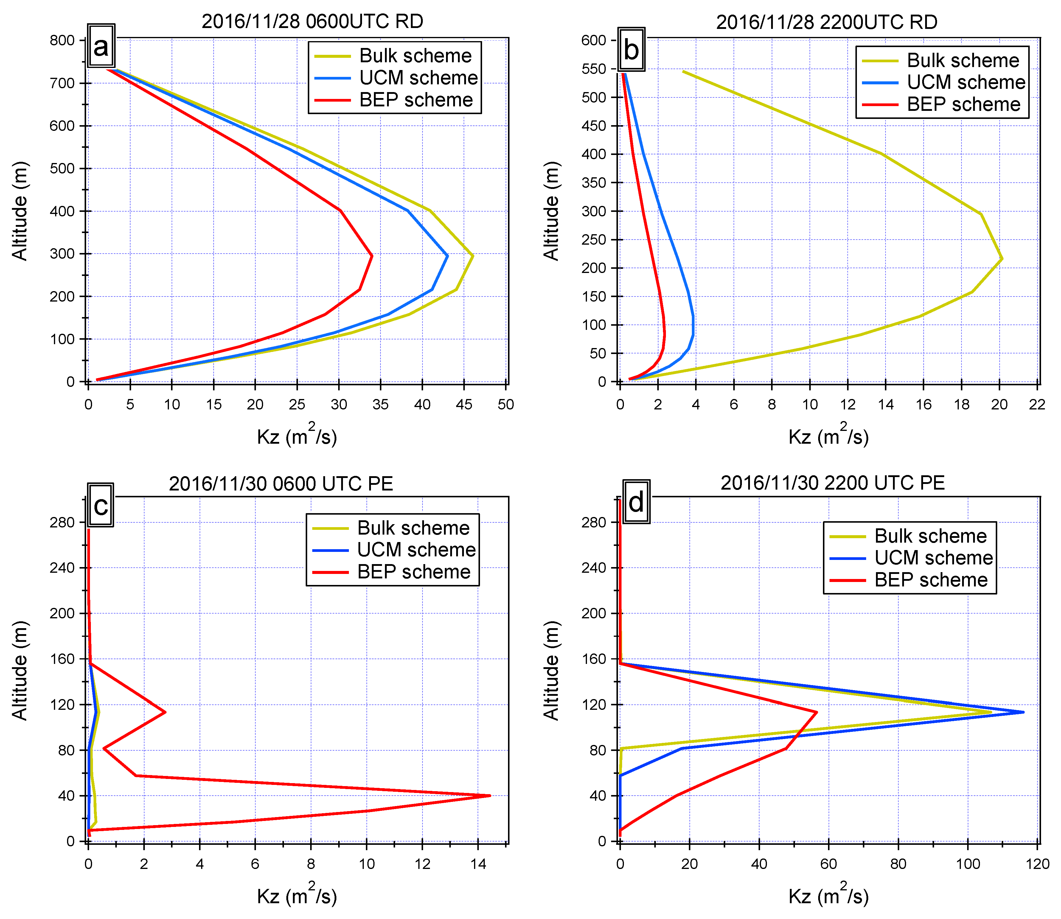
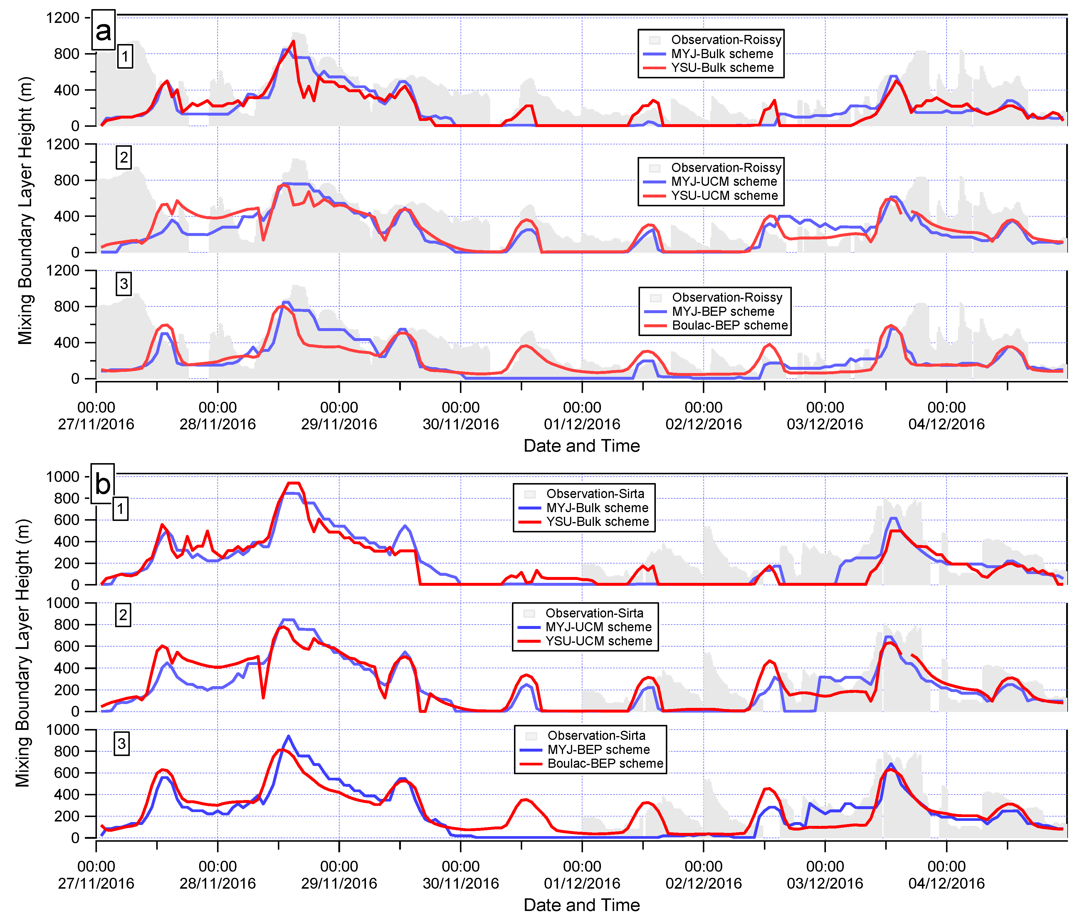
3.3.1. PBL Height

WRF version 3.9.1 provides 14 options for the PBL scheme, following the approach of LeMoine et al. [58,59]. Briefly, they can be categorized as TKE schemes and non-TKE schemes. Two TKE-based schemes and one non-TKE-based PBL scheme are selected for these PBL sensitivity simulations. The TKE schemes chosen in this assessment are the MYJ and Boulac schemes, and the non-TKE scheme is the YSU scheme. Unified PBL sensitivities are not possible in this section with the canopy schemes from the previous section, because the BEP urban canopy scheme requires the simultaneous use of a TKE scheme and the Boulac PBL scheme is designed for coupling with the multi-urban canopy model. Regarding the configuration of the canopy models in Section 3.2, each canopy scheme will be coupled with two PBL schemes, giving the YSU–Bulk and MYJ–Bulk schemes, the YSU–UCM and MYJ–UCM schemes, and the Boulac–BEP and MYJ–BEP schemes. All the other physics options are the same. For the observed PBL height, we have the complete dataset for Roissy station and the last four days data for Sirta station. Figure 14 displays a comparison between the observed Lidar data and the 15 min averaged modeled output of PBL height. Generally, all the PBL schemes systematically underestimate PBL height for the whole time series, especially during the PE and the beginning of RD (from 27th November 00:00 UTC). This explains the strong overestimations of pollutants during the PE in Section 3.2 and is consistent with the positive biases of pollutant concentrations at the beginning of the RD in Figure 10. If we consider the simulation of PBL during the PE, the average observed PBL height was around 110 m and is only relatively well reproduced by the Boulac–BEP, scheme even though it still underestimates the PBL height by around 40 m on average. The other PBL schemes reach the minimum PBL height (set up to 20 m in the model) during the whole PE and strongly underestimate PBL height, especially at night and early in the morning. In general, the Boulac–BEP scheme gives the best performance, and it is the only option which can effectively estimate the evolution of the PBL height during the PE in this sensitivity test. For the other PBL schemes, the agreement between the simulations and observations is poor. MYJ displays the poorest correlation compared to the observed soundings, regardless of other parameter settings.

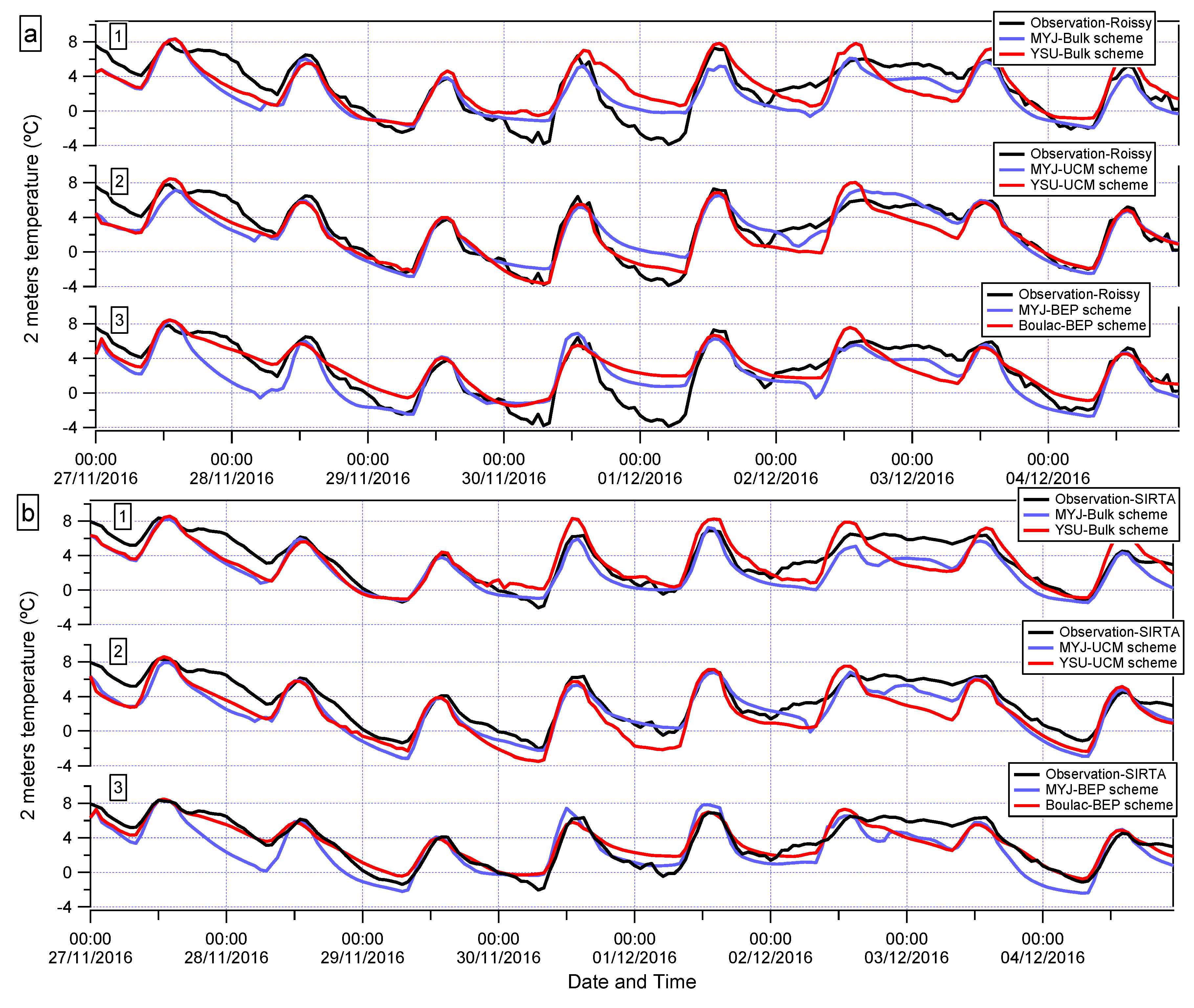
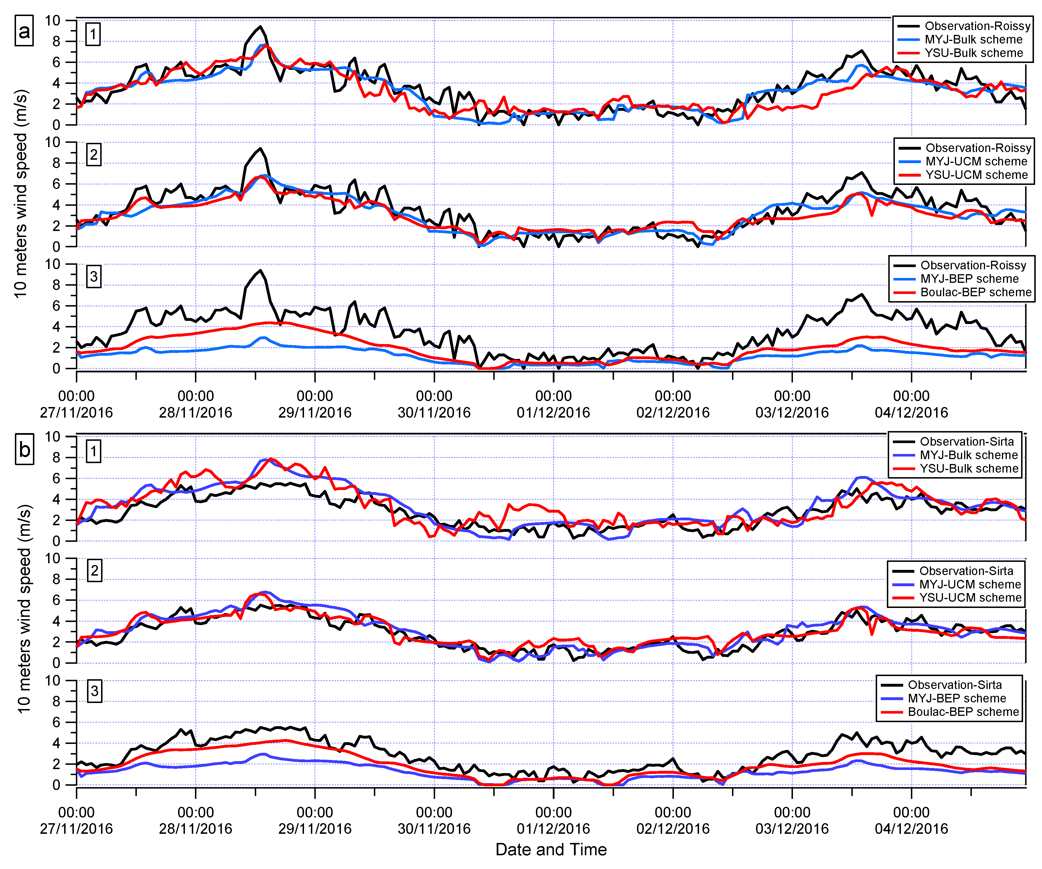
3.3.2. Ground Meteorological Variables

A comparison of the performances of various PBL schemes in simulating the surface meteorological variables (T2 and W10) is presented in this section. Figure 15 and Figure 16 shows the time series of T2 and W10 based on several PBL schemes. The YSU–Bulk and Boulac–BEP have a slight positive bias compared to MYJ, but the YSU–UCM scheme had a cooling effect compared to the MYJ–UCM scheme during the PE. In the MYJ–BEP and Boulac–BEP schemes, it can be observed that the models always underestimate the wind speed compared to the observations in this period. The Boulac–BEP scheme produces a lower W10 than MYJ–BEP throughout the whole period, especially during RD. In contrast, W10 does not show significant differences between the MYJ and YSU schemes coupled with the other two Bulk and UCM canopy models. Table 3 summarizes the performances of the models, including the mean bias (MB) and mean Pearson correlation coefficient (R) of meteorological variables. These schemes display a high correlation which approximately reproduces the measured trend. The three experiments with the MYJ boundary layer scheme display a negative bias in W10 in Roissy and a negative bias in T2 in both Roissy and Sirta stations. A less negative bias is noticed with the simulations using the Boulac–BEP scheme compared with the others for the whole period, but it still produces a positive bias during nighttime in the PE. The reason could be that the Boulac PBL scheme takes the turbulent exchange affected by complex terrain into account in the calculation of the turbulent diffusion coefficient, leading to a smaller bias in T2 prediction [60]. The Boulac–BEP scheme slightly improves the results with respect to the MYJ–BEP scheme for the W10, but still massively underestimates by 1.53 m s−1 at Roissy station. The correlation indicates the PBL schemes coupled with the urban canopy schemes (MYJ–UCM, YSU–UCM, MYJ–BEP, and Boulac–BEP) are more accurate than those with no urban canopy scheme (MYJ–Bulk and YSU–Bulk). In contrast to the PBL height results, the model performances for T2 and W10 based on various PBL schemes are mixed. Therefore, it is not straightforward to agree on a definitive best choice for the PBL scheme.

3.3.3. Air Quality Simulations

The impacts of the PBL schemes on air quality are analyzed in this section. The time series of the model predictions of the NO2, PM2.5, PM10 concentrations for all the schemes are compared with the observations (the NO2 can be found in Figure 17; the PM2.5 and PM10 can be found in Figures S4 and S5). In general, all the schemes have a better performance for the RD than the PE period, and almost all the schemes strongly overestimate pollutant concentrations at the beginning of the PE, except the Boulac–BEP scheme. The bias between the modelled and observed pollutant concentrations can be found in Figures S6–S8. All the schemes give a worse performance for NO2 and PM2.5 prediction than for PM10. The PBL height reaches the minimum value at 18:00 UTC on 29th November, with the YSU–Bulk scheme corresponding to an underestimation of 500 m; such a difference creates a large bias in air pollutant concentrations. The same phenomenon occurs for the MYJ–Bulk, MYJ–UCM, YSU–UCM, and MYJ–BEP schemes at 00:00 UTC on 30th November. However, the overestimation of pollutant concentrations does not occur at this time but at 06:00 UTC on 1st December, because this episode is largely influenced by local sources (road traffic and residential heating). On 1st December 2016 at 06:00 UTC (a weekday), the morning rush hour leads to a lag effect in the bias, explaining why all the schemes have their worst performance for the NO2 and PM2.5 predictions. The averaged statistics for the four air quality monitoring stations are summarized in Table 4. Figure 18 gives the scatterplot between the observed and modelled NO2; the scatterplot for the PM2.5 and PM10 can be found in Figure S9. Overall, the MYJ scheme overestimates the mass concentrations of all pollutants, whatever the selected urban canopy model. The Boulac–BEP scheme has a significantly better performance than other schemes for all the evaluated variables. The YSU–Bulk scheme has the lowest mean bias (−1.3 µg m−3) in PM10 prediction, but its mean linear correlation coefficients of NO2, PM2.5, and PM10 were 0.52, 0.40, and 0.53, respectively. The mean biases for the NO2 and PM2.5 prediction were 17.6 and 46.0 µg m−3, respectively. The low correlation for all the analyzed variables, positive biases for NO2 and PM2.5 prediction, and negative bias for PM10 prediction indicate that this scheme under and over-estimates the concentrations simultaneously, which means that the YSU–Bulk scheme cannot be performed effectively for the prediction of short-term PE in urban regions. The Boulac–BEP scheme was better for all the analyzed variables, both in terms of bias and correlation statistics; its mean biases for NO2, PM2.5, and PM10 prediction were −5.1, 1.2, and −8.6 µg m−3, respectively. This indicates that both the urban canopy and PBL schemes play an important role in the PE forecast for urban regions.

4. Conclusions

This study evaluates the impact of three urban canopy parametrization schemes (Bulk, UCM, and BEP) and three boundary layer parametrization schemes coupled with urban canopy schemes (MYJ–Bulk, YSU–Bulk, MYJ–UCM, YSU–UCM, MYJ–BEP, and Boulac–BEP) from the Weather Research and Forecasting (WRF Version 3.9.1) mesoscale model on the simulations of meteorological variables and predicted pollutant concentrations issued from the CHIMERE chemical transport model. This study aims at understanding those impacts on the short-term pollution episode in the Paris region, France.
For the first time, chemistry transport models have been used with a first layer at 4 m to better account for physical processes within the suburban layer in relation to ground emissions such as road traffic. Clearly, the sharp gradient of concentrations shows the added value of using such a low level in urban areas. This study shows the high sensitivity of air quality simulation to meteorological model outputs during stable conditions favorable to the occurrence of PM episodes.
Three urban canopy models could reproduce the T2 effectively in the daytime; the Bulk and UCM model reproduced the W10 well, but the BEP model underestimates W10 for the whole episode, indicating an important impact of buildings on the diffusion rate for this scheme. The UCM scheme overestimates the surface heat index in rural areas, leading to a slight negative bias for T2 in rural versus urban areas. T2 displays ambiguous results, while all schemes reproduced results well at Sirta station but overestimated during nighttime at Montsouris and Roissy during a pollution episode. This could be due to the use of a single urban category in this study, which leads to a discrepancy that causes more spatial variability in urban parameters. NO2, PM2.5, and PM10 were selected to evaluate the effect of physics parameterizations on air quality simulation. Large differences were found in the simulation of pollutant concentrations, with an overall overestimation during the pollution episode.
The six PBL sensitivity tests display an underestimation of the PBL height when compared with the observations issued from the Lidar. All the sensitivity tests, except Boulac–BEP, could not effectively simulate the PBL height during the pollution episode. The two PBL schemes coupled with the BEP scheme still underestimated the W10 for the whole period, but the Boulac–BEP scheme improved the simulations compared with the MYJ–BEP scheme. The Boulac–BEP scheme had a significantly better performance than the other schemes for the simulation of pollutant concentrations, indicating that both the canopy parametrization and PBL schemes have a positive effect on air quality simulation in urban regions, especially during pollution episodes. An advanced urban category could improve air quality prediction in urban regions.

Supplementary Materials

The following are available online at https://www.mdpi.com/2073-4433/11/6/618/s1: Table S1. The urban parameters for the urban canopy model; Figure S1. Time series of PM2.5, PM10 mass concentrations: No1, 2, 3, 4 represent station FR04002, FR04034, FR04143, FR04156, respectively; Figure S2. Time series of bias of NO2, PM2.5, PM10 mass concentrations: No1, 2, 3, 4 represent station FR002, FR034, FR143, FR156, respectively; Figure S3. Time series between observed and modelled NO2 with the first height of about 4 m, 18 m and 40 m, respectively. Both observation and simulations are the average of Station FR04002, FR04034, FR04143, FR04156, respectively; Figure S4. Time series between observed and modelled PM2.5: a, b and c represent each PBL schemes coupled with each urban canopy schemes respectively; 1, 2, 3, and 4 represent Station FR04002, FR04034, FR04143, FR04156, respectively; Figure S5. Time series between observed and modelled PM10: a, b and c represent each PBL schemes coupled with each urban canopy schemes respectively; 1, 2, 3, and 4 represent Station FR04002, FR04034, FR04143, FR04156, respectively; Figure S6. Time series of bias between observed and modelled NO2: a, b and c represent each PBL schemes coupled with each urban canopy schemes respectively; 1, 2, 3, and 4 represent Station FR04002, FR04034, FR04143, FR04156, respectively; Figure S7. Time series of bias between observed and modelled PM2.5: a, b and c represent each PBL schemes coupled with each urban canopy schemes respectively; 1, 2, 3, and 4 represent Station FR04002, FR04034, FR04143, FR04156, respectively; Figure S8. Time series of bias between observed and modelled PM10: a, b and c represent each PBL schemes coupled with each urban canopy schemes respectively; 1, 2, 3, and 4 represent Station FR04002, FR04034, FR04143, FR04156, respectively; Figure S9. Liner fit between observed and modelled PM2.5 and PM10; List.S1. Name list of WRF model.

Author Contributions

Conceptualization, B.B.; Data curation, L.J.; Formal analysis, L.J.; Funding acquisition, B.B.; Methodology, L.J.; Project administration, B.B.; Software, L.J., B.B. and F.C.; Validation, F.M., F.T. and F.C.; Writing—original draft, L.J.; Writing—review and editing, B.B., F.M., F.T. and F.C. All authors have read and agreed to the published version of the manuscript.

Funding

This work is funded by the French Ministry in charge of Environment (MTES).

Conflicts of Interest

The authors declare no conflict of interest.

References

  1. EEA. Air Quality in Europe—2018 Report; EEA Report No. 13/2018; European Environment Agency: Copenhagen, Denmark, 2018. [Google Scholar]
  2. Sarrat, C.; Lemonsu, A.; Masson, V.; Guedalia, D. Impact of urban heat island on regional atmospheric pollution. Atmos. Environ. 2006, 40, 1743–1758. [Google Scholar] [CrossRef]
  3. Coseo, L. Larsen Cooling the heat island in compact urban environments: The effectiveness of Chicago’s green alley program. Procedia Eng. 2015, 118, 691–710. [Google Scholar] [CrossRef] [Green Version]
  4. Falasca, S.; Catalano, F. Impact of Highly Reflective Materials on Meteorology, PM10 and Ozone in Urban Areas: A Modeling Study with WRF-CHIMERE at High Resolution over Milan (Italy). Urban Sci. 2018, 2, 18. [Google Scholar] [CrossRef] [Green Version]
  5. Lin, C.-Y.; Chen, F.; Huang, J.-C.; Chen, W.-C.; Liou, Y.-A.; Chen, W.-N.; Liu, S.-C. Urban heat island effect and its impact on boundary layer development and land–sea circulation over northern Taiwan. Atmos. Environ. 2008, 42, 5635–5649. [Google Scholar] [CrossRef]
  6. Falasca, S.; Catalano, F.; Moroni, M. Numerical Study of the Daytime Planetary Boundary Layer over an Idealized Urban Area: Influence of Surface Properties, Anthropogenic Heat Flux, and Geostrophic Wind Intensity. J. Appl. Meteorol. Climatol. 2016, 55, 1021–1039. [Google Scholar] [CrossRef]
  7. Gedzelman, S.D.; Austin, S.; Cermak, R.; Stefano, N.; Partridge, S.; Quesenberry, S.; Robinson, D.A. Mesoscale aspects of the Urban Heat Island around New York City. Theor. Appl. Climatol. 2003, 75, 29–42. [Google Scholar] [CrossRef]
  8. Lai, L.-W.; Cheng, W.-L. Air quality influenced by urban heat island coupled with synoptic weather patterns. Sci. Total. Environ. 2009, 407, 2724–2733. [Google Scholar] [CrossRef]
  9. Lin, C.-Y.; Chen, W.-C.; Liu, S.C.; Liou, Y.A.; Liu, G.; Lin, T. Numerical study of the impact of urbanization on the precipitation over Taiwan. Atmos. Environ. 2008, 42, 2934–2947. [Google Scholar] [CrossRef]
  10. Best, M. Representing urban areas within operational numerical weather prediction models. Bound. Layer Meteorol. 2005, 114, 91–109. [Google Scholar] [CrossRef]
  11. Liu, Y.; Chen, F.; Warner, T.; Basara, J.B. Verification of a Mesoscale Data-Assimilation and Forecasting System for the Oklahoma City Area during the Joint Urban 2003 Field Project. J. Appl. Meteorol. Climatol. 2006, 45, 912–929. [Google Scholar] [CrossRef]
  12. Bessagnet, B.; Beauchamp, M.; Guerreiro, C.; De Leeuw, F.; Tsyro, S.; Colette, A.; Meleux, F.; Rouïl, L.; Ruyssenaars, P.; Sauter, F.; et al. Can further mitigation of ammonia emissions reduce exceedances of particulate matter air quality standards? Environ. Sci. Policy 2014, 44, 149–163. [Google Scholar] [CrossRef]
  13. Barlage, M.; Miao, S.; Chen, F. Impact of physics parameterizations on high-resolution weather prediction over two Chinese megacities. J. Geophys. Res. Atmos. 2016, 121, 4487–4498. [Google Scholar] [CrossRef] [Green Version]
  14. Molteni, F.; Buizza, R.; Palmer, T.N.; Petroliagis, T. The ECMWF ensemble prediction system: Methodology and validation. Quart. J. R. Meteor. Soc. 1996, 122, 73–119. [Google Scholar] [CrossRef]
  15. Tuccella, P.; Curci, G.; Visconti, G.; Bessagnet, B.; Menut, L.; Park, R.J. Modeling of gas and aerosol with WRF/Chem over Europe: Evaluation and sensitivity study. J. Geophys. Res. Space Phys. 2012, 117, D03303. [Google Scholar] [CrossRef] [Green Version]
  16. Salamanca, F.; Krpo, A.; Martilli, A.; Clappier, A. A new building energy model coupled with an urban canopy parameterization for urban climate simulations—Part I. formulation, verification, and sensitivity analysis of the model. Theor. Appl. Climatol. 2009, 99, 331–344. [Google Scholar] [CrossRef]
  17. Salamanca, F.; Martilli, A. A new Building Energy Model coupled with an Urban Canopy Parameterization for urban climate simulations—Part II. Validation with one-dimension off-line simulations. Theor. Appl. Climatol. 2009, 99, 345–356. [Google Scholar] [CrossRef]
  18. Miao, S.; Chen, F.; Li, Q.; Fan, S. Impacts of urban processes and urbanization on summer precipitation: A case study of heavy rainfallin Beijing on 1 Aug 2006. J. Appl. Meteorol. Climatol. 2010, 50, 806–825. [Google Scholar] [CrossRef]
  19. Fan, S.; Guo, Y.R.; Chen, M.; Zhong, J.; Chu, Y.; Wang, W.; Huang, X.Y.; Wang, Y.; Guo, Y.H. Application of WRF 3D Var to a high-resolution model over Beijing area. Plateau Meteorol. 2008, 27, 1181–1188. [Google Scholar]
  20. Liu, M.; Chen, M. Evaluation of BJ-RUC system for the forecast quality of planetary boundary layer in Beijing area. J. Appl. Meteorol. Sci. 2014, 25, 212–221. [Google Scholar]
  21. Valari, M.; Menut, L. Transferring the heterogeneity of surface emissions to variability in pollutant concentrations over urban areas through a chemistry-transport model. Atmos. Environ. 2014, 44, 3229–3238. [Google Scholar] [CrossRef]
  22. Markakis, K.; Valari, M.; Engardt, M.; Lacressonniere, G.; Vautard, R.; Andersson, C. Mid-21st century air quality at the urban scale under the influence of changed climate and emissions case studies for Paris and Stockholm. Atmos. Chem. Phys. 2016, 16, 1877–1894. [Google Scholar] [CrossRef] [Green Version]
  23. He, Q.; Zhao, X.; Lu, J.; Zhou, G.; Yang, H.; Gao, W.; Yu, W.; Cheng, T. Impacts of biomass-burning on aerosol properties of a severe haze event over Shanghai. Particuology 2015, 20, 52–60. [Google Scholar] [CrossRef]
  24. Wang, L.T.; Wei, Z.; Yang, J.; Zhang, Y.; Zhang, F.F.; Su, J.; Meng, C.C.; Zhang, Q. The 2013 severe haze over southern Hebei, China: Model evaluation, source apportionment, and policy implications. Atmos. Chem. Phys. Discuss. 2014, 14, 3151–3173. [Google Scholar] [CrossRef] [Green Version]
  25. Wang, L.; Liu, J.; Gao, Z.; Li, Y.; Huang, M.; Fan, S.; Zhang, X.; Yang, Y.; Miao, S.; Zou, H.; et al. Vertical observations of the atmospheric boundary layer structure over Beijing urban area during air pollution episodes. Atmos. Chem. Phys. Discuss. 2019, 19, 6949–6967. [Google Scholar] [CrossRef] [Green Version]
  26. Hu, X.-M.; Nielsen-Gammon, J.W.; Zhang, F. Evaluation of Three Planetary Boundary Layer Schemes in the WRF Model. J. Appl. Meteorol. Climatol. 2010, 49, 1831–1844. [Google Scholar] [CrossRef] [Green Version]
  27. Hariprasad, K.B.R.R.; Srinivas, C.V.; Singh, A.B.; Rao, S.V.B.; Baskaran, R.; Venkatraman, B. Numerical simulation and inter comparison of boundary layer structure with different PBL schemes in WRF using experimental observations at a tropical site. Atmos. Res. 2014, 145, 27–44. [Google Scholar] [CrossRef]
  28. Tyagi, B.; Magliulo, V.; Finardi, S.; Gasbarra, D.; Carlucci, P.; Toscano, P.; Zaldei, A.; Riccio, A.; Calori, G.; D’Allura, A.; et al. Performance Analysis of Planetary Boundary Layer Parameterization Schemes in WRF Modeling Set Up over Southern Italy. Atmosphere 2018, 9, 272. [Google Scholar] [CrossRef] [Green Version]
  29. Kleczek, M.A.; Steeneveld, G.-J.; Holtslag, A. Evaluation of the Weather Research and Forecasting Mesoscale Model for GABLS3: Impact of Boundary-Layer Schemes, Boundary Conditions and Spin-Up. Bound. Layer Meteorol. 2014, 152, 213–243. [Google Scholar] [CrossRef]
  30. Borrego, C.; Souto, J.A.; Monteiro, A.; Dios, M.; Rodriguez, A.; Ferreira, J.; Saavedra, S.; Casares, J.J.; Miranda, A.I. The role of transboundary air pollution over Galicia and North Portugal area. Environ. Sci. Pollut. Res. 2013, 20, 2924–2936. [Google Scholar] [CrossRef]
  31. Anderson, W.; Meneveau, C. A Large-Eddy Simulation Model for Boundary-Layer Flow over Surfaces with Horizontally Resolved but Vertically Unresolved Roughness Elements. Bound. Layer Meteorol. 2010, 137, 397–415. [Google Scholar] [CrossRef]
  32. Martilli, A.; Clappier, A.; Rotach, M. An urban surface exchange parameterization for mesoscale models. Bound. Layer Meteorol. 2002, 104, 261–304. [Google Scholar] [CrossRef]
  33. Flaounas, E.; Bastin, S.; Janicot, S. Regional climate modelling of the 2006 West African monsoon: Sensitivity to convection and planetary boundary layer parameterisation using WRF. Clim. Dyn. 2010, 36, 1083–1105. [Google Scholar] [CrossRef]
  34. Patricola, C.M.; Li, M.; Xu, Z.; Chang, P.; Saravanan, R.; Hsieh, J.-S. An investigation of tropical Atlantic bias in a high-resolution coupled regional climate model. Clim. Dyn. 2012, 39, 2443–2463. [Google Scholar] [CrossRef]
  35. Vigaud, N.; Roucou, P.; Fontaine, B.; Sijikumar, S.; Tyteca, S. WRF/ARPEGE-CLIMAT simulated climate trends over West Africa. Clim. Dyn. 2009, 36, 925–944. [Google Scholar] [CrossRef]
  36. Bowden, J.H.; Otte, T.L.; Nolte, C.G.; Otte, M. Examining Interior Grid Nudging Techniques Using Two-Way Nesting in the WRF Model for Regional Climate Modeling. J. Clim. 2012, 25, 2805–2823. [Google Scholar] [CrossRef]
  37. Glisan, J.M.; Gutowski, W.J.; Cassano, J.J.; Higgins, M.E. Effects of Spectral Nudging in WRF on Arctic Temperature and Precipitation Simulations. J. Clim. 2013, 26, 3985–3999. [Google Scholar] [CrossRef]
  38. Kusaka, H.; Kondo, K.; Kikegawa, Y.; Kimura, F. A simple single-layer urban canopy model for atmospheric models: Comparison with multi-layer and slab models. Bound. Layer Meteorol. 2001, 101, 329–358. [Google Scholar] [CrossRef]
  39. Kusaka, H.; Kimura, F. Coupling a Single-Layer Urban Canopy Model with a Simple Atmospheric Model: Impact on Urban Heat Island Simulation for an Idealized Case. J. Meteorol. Soc. Jpn. 2004, 82, 67–80. [Google Scholar] [CrossRef] [Green Version]
  40. Mellor, G.L.; Yamada, T. Development of a turbulence closure model for geophysical fluid problems. Rev. Geophys. 1982, 20, 851–875. [Google Scholar] [CrossRef] [Green Version]
  41. Janjic, Z. Nonsingular Implementation of the Mellor-Yamada Level 2.5 Scheme in the NCEP Meso Model; NCEP Office Note, No. 437; National Centers for Environmental Prediction: College Park, MD, USA, 2002; p. 61. [Google Scholar]
  42. Janjić, Z.I. The Step-Mountain Coordinate: Physical Package. Mon. Weather Rev. 1990, 118, 1429–1443. [Google Scholar] [CrossRef]
  43. Hong, S.-Y.; Noh, Y.; Dudhia, J. A New Vertical Diffusion Package with an Explicit Treatment of Entrainment Processes. Mon. Weather Rev. 2006, 134, 2318–2341. [Google Scholar] [CrossRef] [Green Version]
  44. Bougeault, P.; Lacarrère, P. Parameterization of orographic induced turbulence in a meso beta scale model. Mon. Weather Rev. 1989, 117, 1872–1890. [Google Scholar] [CrossRef]
  45. Menut, L.; Bessagnet, B.; Khvorostyanov, D.; Beekmann, M.; Blond, N.; Colette, A.; Coll, I.; Curci, G.; Forêt, G.; Hodzic, A.; et al. CHIMERE 2013: A model for regional atmospheric composition modelling. Geosci. Model Dev. 2013, 6, 981–1028. [Google Scholar] [CrossRef] [Green Version]
  46. Troen, I.B.; Mahrt, L. A simple model of the atmospheric boundary layer; sensitivity to surface evaporation. Bound. Layer Meteorol. 1986, 37, 129–148. [Google Scholar] [CrossRef]
  47. Bessagnet, B.; Hodzic, A.; Vautard, R.; Beekmann, M.; Cheinet, S.; Honoré, C.; Liousse, C.; Rouil, L. Aerosol modeling with CHIMERE—preliminary evaluation at the continental scale. Atmos. Environ. 2004, 38, 2803–2817. [Google Scholar] [CrossRef]
  48. Menut, L.; Goussebaile, A.; Bessagnet, B.; Khvorostiyanov, D.; Ung, A. Impact of realistic hourly emissions profiles on air pollutants concentrations modelled with CHIMERE. Atmos. Environ. 2012, 49, 233–244. [Google Scholar] [CrossRef]
  49. Bessagnet, B.; Menut, L.; Colette, A.; Couvidat, F.; Dan, M.; Mailler, S.; Létinois, L.; Pont, V.; Rouïl, L. An Evaluation of the CHIMERE Chemistry Transport Model to Simulate Dust Outbreaks across the Northern Hemisphere in March 2014. Atmosphere 2017, 8, 251. [Google Scholar] [CrossRef] [Green Version]
  50. Mailler, S.; Menut, L.; Khvorostyanov, D.; Valari, M.; Couvidat, F.; Siour, G.; Turquety, S.; Briant, R.; Tuccella, P.; Bessagnet, B.; et al. CHIMERE-2017: From urban to hemispheric chemistry-transport modeling. Geosci. Model Dev. 2017, 10, 2397–2423. [Google Scholar] [CrossRef] [Green Version]
  51. Couvidat, F.; Bessagnet, B.; Garcia-Vivanco, M.; Real, E.; Menut, L.; Colette, A. Development of an inorganic and organic aerosol model (Chimere2017b2 v1.0): Seasonal and spatial evaluation over Europe. Geosci. Model. Dev. 2018, 11, 165–194. [Google Scholar] [CrossRef] [Green Version]
  52. Kim, Y.; Sartelet, K.; Raut, J.-C.; Chazette, P. Influence of an urban canopy model and PBL schemes on vertical mixing for air quality modeling over Greater Paris. Atmos. Environ. 2015, 107, 289–306. [Google Scholar] [CrossRef] [Green Version]
  53. Allen, L.; Lindberg, F.; Grimmond, C.S.B. Global to city scale urban anthropogenic heat flux: Model and variability. Int. J. Climatol. 2010, 31, 1990–2005. [Google Scholar] [CrossRef]
  54. Kim, Y.; Sartelet, K.; Raut, J.-C.; Chazette, P. Evaluation of the Weather Research and Forecast/Urban Model over Greater Paris. Bound. Layer Meteorol. 2013, 149, 105–132. [Google Scholar] [CrossRef] [Green Version]
  55. Wul, J.; Zha, J.L.; Zhao, D.M.; Yang, Q.D. Changes in terrestrial near-surface wind speed and their possible causes: An overview. Clim. Dyn. 2017, 51, 2039–2078. [Google Scholar]
  56. Toll, I.; Baldasano, J.M. Modeling of photochemical air pollution in the Barcelona area with highly disaggregated anthropogenic and biogenic emissions. Atmos. Environ. 2000, 34, 3069–3084. [Google Scholar] [CrossRef]
  57. Baklanov, A.; Mestayer, P.G.; Clappier, A.; Zilitinkevich, S.; Joffre, S.; Mahura, A.; Nielsen, N.W. Towards improving the simulation of meteorological fields in urban areas through updated/advanced surface fluxes description. Atmos. Chem. Phys. Discuss. 2008, 8, 523–543. [Google Scholar] [CrossRef] [Green Version]
  58. LeMone, M.; Tewari, M.; Chen, F.; Dudhia, J. Objectively-determined fair-weather convective boundary layer depths in the ARW-WRF NWP model and their comparison to CASES-97 observations. Mon. Weather Rev. 2013, 141, 30–54. [Google Scholar] [CrossRef] [Green Version]
  59. LeMone, M.; Tewari, M.; Chen, F.; Dudhia, J. Objectively-determined fair-weather NBL features in the ARW-WRF model and their comparison to CASES-97 observations. Mon. Weather Rev. 2014, 142, 2709–2732. [Google Scholar] [CrossRef] [Green Version]
  60. Li, M.; Ma, Y.; Ma, W.; Hu, Z.; Ishikawa, H.; Su, Z.; Sun, F. Analysis of turbulence characteristics over the northern Tibetan Plateau area. Adv. Atmos. Sci. 2006, 23, 579–585. [Google Scholar] [CrossRef]
Figure 1. Four nested domains—from d01, the largest one, at a low resolution to d04, the finest one, at a high resolution.
Atmosphere 11 00618 g001
Figure 2. Maps of the meteorological and air quality monitoring stations.
Atmosphere 11 00618 g002
Figure 3. Time series of 2 m temperature and 10 m wind speed at Sirta station.
Atmosphere 11 00618 g003
Figure 4. Time series of 2 m temperature and 10 m wind speed at Montsouris station.
Atmosphere 11 00618 g004
Figure 5. Maps of the mean 2 m temperature (°C) over the period from 27th November to 4th December.
Atmosphere 11 00618 g005
Figure 6. Maps of the mean surface heat flux (W m−2) over the period from 27th November to 4th December.
Atmosphere 11 00618 g006
Figure 7. Time series of 2 m temperature (°C) between observations and different urban schemes at Montsouris, Roissy, and Sirta stations.
Atmosphere 11 00618 g007
Figure 8. Maps of the mean 10 m wind speed (m s−1) over the period from 27th November to 4th December.
Atmosphere 11 00618 g008
Figure 9. Comparison of the time series of 10 m wind speed (m s−1) between the observations and different urban schemes at Montsouris, Roissy and Sirta stations.
Atmosphere 11 00618 g009
Figure 10. The differences in the daily averaged NO2 (μg m−3), PM2.5 (μg m−3), and PM10 (μg m−3) between different schemes from 27th November to 4th December 2016.
Atmosphere 11 00618 g010
Figure 11. Time series of NO2 mass concentrations (µg m−3). No1, 2, 3, 4 represent station FR04002, FR04034, FR04143, and FR04156, respectively.
Atmosphere 11 00618 g011
Figure 12. Vertical profiles of the CHIMERE Kz extracted at the FR04143 station. The profile is extracted at 06:00 and 22:00 UTC for both Regular Days (RD) and the Particulate Episode (PE).
Atmosphere 11 00618 g012
Figure 13. Vertical profiles of the NO2 and PM2.5 mass concentration (µg m−3) at the FR04143 station. The profiles are extracted at 06:00 and 22:00 UTC for both Regular Days (RD) and the Particulate Episode (PE). Columns (a), (b), (c), and (d) represent the vertical mass concentration of NO2 and PM2.5 at 28th November 06:00, 28th November 22:00, 30th November 06:00, and 30th November 22:00 UTC, respectively.
Atmosphere 11 00618 g013
Figure 14. Time series of the observed and modelled mixing boundary layer height: (a) and (b) represent Roissy and Sirta station, respectively; 1, 2, and 3 represent each PBL scheme coupled with each urban canopy scheme.
Atmosphere 11 00618 g014
Figure 15. Time series between the observed and modelled T2: (a) and (b) represent Roissy and Sirta station, respectively; 1, 2, and 3 represent each PBL scheme coupled with each urban canopy scheme.
Atmosphere 11 00618 g015
Figure 16. Time series between the observed and modelled W10: (a) and (b) represent Roissy and Sirta station, respectively; 1, 2, and 3 represent each PBL scheme coupled with each urban canopy scheme.
Atmosphere 11 00618 g016
Figure 17. Time series of NO2 mass concentrations: No 1, 2, 3, and 4 represent station FR04002, FR04034, FR04143, and FR04156, respectively.
Atmosphere 11 00618 g017aAtmosphere 11 00618 g017b
Figure 18. Liner fit between the observed and modelled NO2.
Atmosphere 11 00618 g018
Table 1. Summary of the physics parameterizations used a.
LWSWSLLSURBBL
BULKRRTMGRRTMGMONoahNoMYJ
UCMRRTMGRRTMGMONoahUCMMYJ
BEPRRTMGRRTMGMONoahBEPMYJ
MYJ-BULKRRTMGRRTMGMONoahNoMYJ
YSU-BULKRRTMGRRTMGMONoahNoYSU
MYJ-UCMRRTMGRRTMGMONoahUCMMYJ
YSU-UCMRRTMGRRTMGMONoahUCMYSU
MYJ-BEPRRTMGRRTMGMONoahBEPMYJ
BOULAC-BEPRRTMGRRTMGMONoahBEPBoulac
a LW = longwave radiation; SW = shortwave radiation; SL = surface layer; LS = land surface; URB = urban canopy; BL = boundary layer; RRTMG = rapid radiative transfer model for GCMs scheme; MO = Monin–Obukhov scheme; UCM = single-layer urban canopy scheme; BEP = multi-layer urban canopy scheme; MYJ = Mellor–Yamada–Janjic scheme; YSU = Yonsei University scheme; Boulac = Bougeault and Lacarrere scheme.
Table 2. Statistics of surface pollutants: mean bias between the simulations and observations of NO2, PM2.5, and PM10 during Whole Period (WP) and Pollution Episode (PE).
BulkUCMBEP
WPPEWPPEWPPE
NO221.540.929.862.218.429.7
PM2.521.831.424.937.719.121.1
PM1012.613.715.218.910.14.2
Table 3. Statistics of surface variables: mean bias (MB) and mean linear correlation coefficient (R) between the simulations and observations of 2 m temperature (T2) and 10 m wind speed (W10) at Roissy and Sirta stations.
RoissySirta
T2W10T2W10
MBRMBRMBRMBR
MYJ-Bulk−0.690.83−0.290.86−1.130.880.530.84
YSU-Bulk0.230.77−0.300.780.200.820.620.74
MYJ-UCM−0.220.90−0.380.87−1.080.900.240.91
YSU-UCM−0.510.92−0.460.90−1.310.930.180.88
MYJ-BEP−0.560.82−2.230.89−0.890.86−1.520.90
Boulac-BEP0.400.84−1.530.88−0.030.90−0.900.92
Table 4. Statistics of surface variables: mean bias (MB), root mean square error (RMSE), and mean linear correlation coefficient (R) between the simulations and observations of NO2, PM2.5, PM10.
NO2PM2.5PM10
MBRRMSEMBRRMSEMBRRMSE
MYJ-Bulk19.10.773.4021.90.742.3712.50.772.39
YSU-Bulk17.60.521.2846.00.401.12−1.30.532.34
MYJ-UCM29.60.732.2124.90.602.0715.20.642.01
YSU-UCM14.60.762.0315.20.641.885.60.681.93
MYJ-BEP20.00.802.3519.20.721.9110.10.761.93
Boulac-BEP−5.10.792.931.20.741.70−8.60.761.71

