Article

Why Does Fog Deepen? An Analytical Perspective

by
Jonathan G. Izett
* and
Bas J. H. van de Wiel
Department of Geoscience and Remote Sensing, Delft University of Technology, Stevinweg 1, 2628 CN Delft, The Netherlands
*
Author to whom correspondence should be addressed.
Atmosphere 2020, 11(8), 865; https://doi.org/10.3390/atmos11080865
Submission received: 24 April 2020 / Revised: 12 August 2020 / Accepted: 13 August 2020 / Published: 14 August 2020
(This article belongs to the Special Issue Observation, Simulation and Predictability of Fog )

Abstract

:
The overall depth of a fog layer is one of the important factors in determining the hazard that a fog event presents. With discrete observations and often coarse numerical grids, however, fog depth cannot always be accurately determined. To address this, we derive a simple analytical relation that describes the change in depth of a fog interface with time, which depends on the tendencies and vertical gradients of moisture. We also present a lengthscale estimate for the maximum depth over which mixing can occur in order for the fog layer to be sustained, assuming a uniform mixing of the vertical profiles of temperature and moisture. Even over several hours, and when coarse observational resolution is used, the analytical description is shown to accurately diagnose the depth of a fog layer when compared against observational data and the results of large-eddy simulations. Such an analytical description not only enables the estimation of sub-grid or inter-observation fog depth, but also provides a simple framework for interpreting the evolution of a fog layer in time.

1. Introduction

This manuscript presents an analytical description of fog growth and evolution. We do this with two goals: (1) to provide a simple framework for understanding the evolution of fog layers, and (2) to allow for continuous estimation of fog depth and growth rate in otherwise discrete settings.
Fog is a hazard to human activities, especially transportation. As a result, accurate monitoring and forecasting of fog events is essential. In addition to knowing the timing of events, it is important to know the severity of the event, including the depth of the fog layer. For example, the hazard that a shallow fog layer presents to airport operations is much less than that of a deeper fog layer. The dynamics and lifecycle of fog, particularly radiation fog, are also dependent on the depth that the fog layer achieves (see, e.g., in [1]). Shallow fog, for example, is optically thin, allowing longwave radiation to pass through without significant absorption, while deeper fog layers (on the order of a few tens of meters) can be optically thick to longwave radiation, resulting in a well-mixed, convective fog layer. Understanding how, at what rate, and why a shallow fog layer transitions to a deep layer is therefore essential. It has been shown that very shallow (<1 m) fog layers can exist long before the evolution, and even in the absence of a deeper fog layer [2]. The need to identify when—and why—these fog layers ultimately deepen was highlighted as an important follow-up.
Unfortunately, accurately characterizing fog depth—observationally or through simulation—is not always straightforward. Continuous resolution is unattainable due to the discretization of observational and numerical systems. Standard observational sites are limited to only a few discrete sensor heights; while fog can be observed at the discrete heights, providing a range of possible depths, the rate of progress between two observational levels cannot be characterized. Higher resolution observations can, of course, be made; however, it becomes impractical in many settings. In an attempt to overcome observational limitations, near-surface micrometeorological observations have been previously employed to estimate fog depth, including in [3,4] and the references therein. Such methods rely on statistical relations between primarily surface parameters and resulting fog depth. Ju et al. The authors of [4] investigate the effectiveness of such methods, and find that they provide a good estimate of the mean height of fog layers. The statistical relationships, however, are site-dependent, only provide an idea of the expected depth, and do not allow for a simple means of estimating a rate of deepening or erosion of the fog top. We therefore seek a general description of the fog-top evolution through means of simple analytical analysis of the fog interface.
Where high-resolution numerical models and diagnostic methods can provide estimates of fog depth and evolution, a conceptual approach also allows for understanding the natural evolution of a fog layer. For example, through an analytical framework, it becomes easier to understand why fog in one stage of its lifecycle is more vulnerable to dissipation than in other stages or to understand why the growth of radiation fog tends to accelerate in time, while optically thick fog typically slows down its own growth, and with higher vulnerability to base-lifting as time proceeds. Previous efforts to understand fog-top evolution have focused on specific processes, such as turbulent mixing and surface characteristics (see, e.g., in [1,5,6]) and their ultimate influence on the overall depth of the fog layer. In contrast, we aim at a simple formula that takes the effect (e.g., interfacial cooling) of the process into account, but without explicit consideration of specific processes. This enables a general understanding of the lifecycle that can be applied in a range of settings.
In Section 2, we derive an analytical description for the rate of deepening or erosion of the fog interface from a Lagrangian perspective. We then compare this with observational data (Section 3) from the campaign of [2], as well as output from simplified large-eddy simulations (LES; Section 4) based on the case described in [5], in order to test the accuracy of the description. With the results presented herein, it becomes possible to provide insight into the immediate evolution of a fog layer as well as quickly and easily diagnose fog depth between standard observation levels. We elaborate further upon these two aspects in the discussion in Section 5.

2. An Analytical Description for the Interface of a Saturated Layer

In this section, an analytical description for the growth (or erosion) rate of the fog interface is presented, providing a means of diagnosing the location and evolution of the interface, even when observational and simulation resolution my be insufficient. In order to maintain generality and simplicity, we approach from the view that cooling and mixing are taking place at the interface, but do not consider specific processes leading to the evolution; the exact processes and their influence will depend on the specific conditions under which the fog has evolved. Our analysis is performed from a localized perspective, focused primarily at the fog interface itself.
We also present a further metric, the “Maximum Attainable Mixed Depth” (MAMD), a lengthscale measure indicating the depth to which a fog layer could extend if the profiles of temperature and moisture were redistributed as well-mixed profiles. A fog layer that is closer to this depth with be more sensitive to drying and mixing influences, than one in otherwise similar conditions that is further from MAMD.

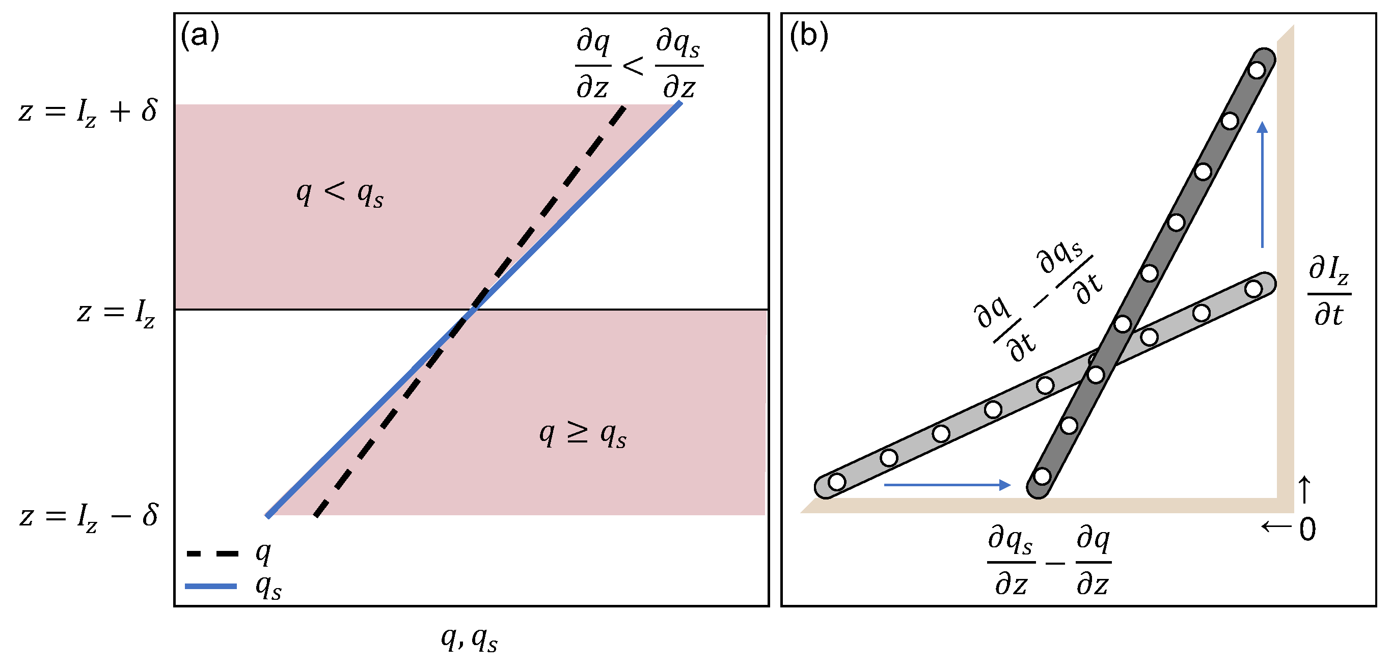
2.1. Derivation of Interfacial Evolution

At the saturation interface of a fog layer ( I z in m), the total specific humidity (q in kg kg 1 ) is by definition equal to the saturation specific humidity ( q s ).
q = q s
For simplicity, we assume this to be the point of 100% relative humidity; however, it could, e.g., be adjusted for microphysical effects, or the threshold at which sufficient liquid water has condensed to reduce visibility to foggy conditions. q s is estimated from the saturation vapor pressure, e s .
q s = R d R v e s p + e s R d R v 1 .
R d and R v are the dry and wet gas constants, respectively, and p is the atmospheric pressure in Pa. e s is then
e s = e s , 0 exp A T 273.15 T B ,
with T the (absolute) air temperature and e s , 0 = 610.87 Pa. A and B are constants, with A = 17.62 and B = 30.03 K when T 273.15 K, and A = 22.46 and B = 0.53 K when T < 273.15 K. The above equations can be found in the majority of meteorological textbooks, including in [7].
Because the air below the interface is saturated, and unsaturated above, it must be true that, at the interface itself,
q s z > q z .
If the values were equal, then the saturated layer would be deeper than the assumed interface. At the same time, a reversal of the inequality represents the lower interface of a cloud above clear air. In the case of fog, this is the surface or the lower interface ( B z ) of a lifted fog layer (e.g., at sunrise).
Figure 1a illustrates this. Given a hypothetical profile for q s at the interface, Equation (4) must be true at the interface itself (but not necessarily at a distance), and fog can exist if q is in the shaded regions. However, if these assumptions are not met, then fog is not present. For example, if q q s up to a height that is greater than I z , then either a deeper fog layer is present (i.e., not assessing at the interface) or a lifted cloud is present.
We can assess the change in interfacial values of q and q s from a Lagrangian perspective, by taking the total derivatives of q and q s at z = I z ,
d q d t I z = q t + q z I z t d q s d t I z = q s t + q s z I z t .
We assume that the profiles are in a quasi-steady state such that (relative) moistening is the same on either side of the interface.
For Equations (1) and (4) to be satisfied at t = t 0 + Δ t and a height of I z , then it must be true for the total derivatives that d q d t I z = d q s d t I z , such that
q t + q z I z t = q s t + q s z I z t
Rearranging, the interfacial growth/erosion can be written as
I z t = q t q s t q s z q z 1 .
The definition provided in Equation (4) means the denominator will always be positive in the case of a fog layer. Therefore, the growth, maintenance, or erosion of the fog top depends on the interfacial values of q s / t and q / t :
q t q s t > 0 : Growth = 0 : Maintenance < 0 : Erosion .
The exact values of the moistening will depend on the specific processes involved, and can be diagnosed either through observations, or through a more detailed budget analysis of the interface. It is important to note that, while the approach is different, this result does not contradict the mixing analysis of the work in [6]; the resulting saturation of the fog layer must be maintained or enhanced for fog to grow. Further, the greater the relative moistening, the more rapidly the growth can occur.
Two further conclusions can be drawn regarding the denominator. First, q s z q z at the interface. Otherwise, there would be infinite growth or erosion. Similarly, the difference between q s z and q z modulates the growth of the fog layer, with a greater difference leading to a slower rate of change. The concept can be thought of as similar to moving up and down a ladder placed against a wall (Figure 1b). The length traveled along the ladder is the numerator, the horizontal base is the denominator, and the vertical axis is I z / t . If placed at a shallow angle against a wall (large denominator), it takes many more steps to climb to the same height as if the ladder were more steeply angled (small denominator).
Important to note is that the relationship does not only hold for the case of a fog layer, but the interface of any saturated region. In the case of a lifted cloud, both the upper and lower interfaces can be described with Equation (7). The only difference is that the sign of the denominator will be negative at the lower interface, as the inequality in Equation (4) is reversed. This, by extension, means that subsidence and lifting of the cloud base, B z , correspond to situations where the numerator is positive and negative, respectively (cf. Equation (8)).
In the following we present idealized examples of Equation (7). Section 2.1.1 illustrates the case of constant moisture, and Section 2.1.2 illustrates a stably stratified log-linear temperature profile.

2.1.1. Equation (7) in the Case of Constant Moisture

To demonstrate the principles of Equation (7), we present a simple illustration of the special case where q / t = q / z = 0 (i.e., the total specific humidity is constant in height and time) and the air cools at a constant rate. Equation (7) then simply becomes
I z t = q s t q s z 1 = T t T z 1 ,
as q s depends only on z and t through the temperature. Then, trivially, I z t = t · T t T z 1 + I z , 0 .
We obtain, then, the intuitive case that the rate of growth or erosion depends on whether or not cooling is occurring at the interface, and the steepness of the temperature gradient is responsible for modulating the overall growth of the fog layer. A steeper gradient means slower growth or erosion than a shallower gradient, which can evolve much more rapidly for for the same cooling rate (Figure 1b).

2.1.2. Equation (7) in a Stable Boundary Layer

One can further assume a stable temperature profile, as might occur during a radiation fog event. We take a simple log-linear profile of temperature in the nocturnal boundary layer, such as would arise from the Businger–Dyer relationship (see, e.g., in [8]), for which the vertical gradient of temperature is given by
T z = θ * κ z 1 + z α L
where θ * is the temperature scale, κ the von Kármán constant, α the linear slope parameter (∼5 under stable conditions), and L the Obukhov length scale. Assuming a quasi-steady state, with T / t constant over the boundary layer, the growth rate at z = I z can be expressed, following Equation (9), as
I z t = T t κ I z L θ * L + I z α
Figure 2 illustrates the (non-dimensional) growth rate as a function of (non-dimensional) fog depth (Equation (11)). Two things are apparent: First, the growth rate accelerates with fog depth (due to the shallower vertical gradient in T), meaning that the second derivative of I z is positive. Second, there is a maximum attainable growth rate for such a profile, which becomes asymptotically linear at large z. We can diagnose this maximum growth rate by taking the limit as I z
max I z t = T t κ L θ * α
If we assume that T / t = 1 K h 1 , L = 10 m, and θ * = 0.1 K, then the fog layer would deepen at rates of 1.6 m h 1 and 6.7 m h 1 at depths of 0.5 m and 10 m, respectively. The maximum growth rate would be 8 m h 1 .

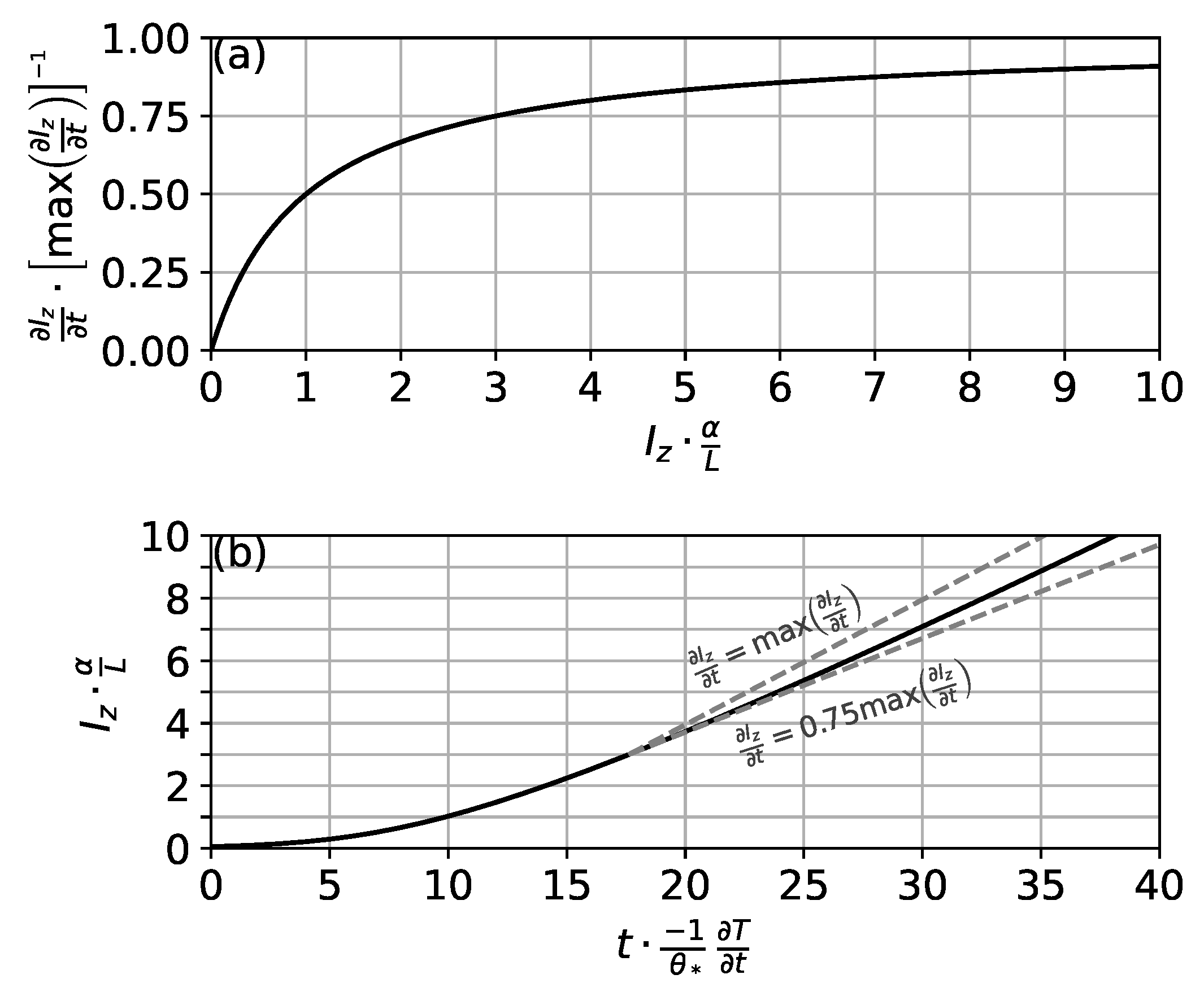
2.2. The Maximum Attainable Mixed Depth
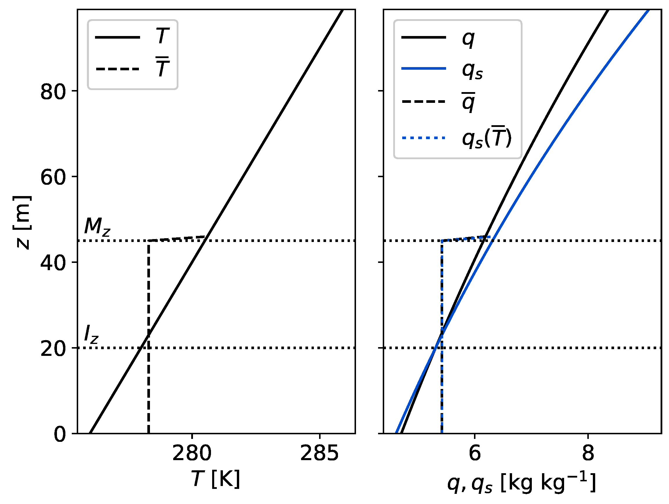
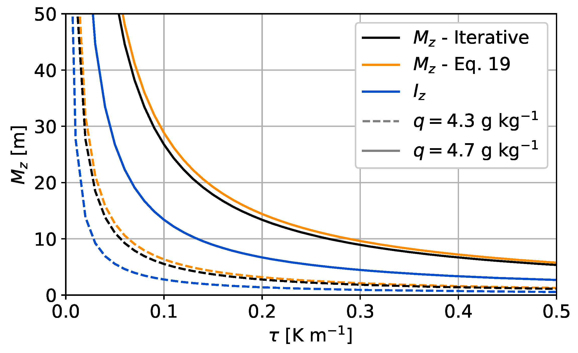
Here, we coin an additional metric to describe a fog layer, the “Maximum Attainable Mixed Depth” (MAMD), or, M z . One can imagine taking a shallow, non-well-mixed fog layer, and identifying the depth to which an equivalent well-mixed fog layer would reach (i.e., redistribute the profiles of q and T equally such that the saturated layer is deeper). This is akin to determining the depth to which a sudden mixing event, or transition from optically thin to optically thick fog, might obtain. MAMD is not a true depth of the fog layer, but rather a thermodynamic lengthscale that describes the amount of moisture available in a vertical profile. As such, the MAMD provides both a hypothetical upper limit of fog depth, as well as an indication of the depth over which mixing can occur and a fog layer still be sustained. Mixing over a deeper layer than M z will result in dissipation of the fog as there is insufficient moisture to maintain saturation. Likewise, if the layer were to dry through, e.g., advection or warming, then MAMD would decrease below the current fog depth, and dissipation would need to occur.
M z is determined through conservation of thermal energy and total specific humidity
0 M z ρ T d z = ρ ¯ T ¯ M z 0 M z q d z = q ¯ M z ,
where the overline represents the well-mixed properties, which are the mean values in the layer
T ¯ = 0 M z ρ T d z ρ ¯ M z q ¯ = 0 M z q d z M z .
The well-mixed profile must also be (super)saturated throughout the layer, adhering to the conditions of Equations (1) and (4), with q ¯ q s T ¯ over the entire M z . Note, we assume complete mixing over the entire M z , with the fog layer being mixed into the air above, such that M z will only be deeper than I z by as much as the supersaturation within the fog layer allows.
Unfortunately, it is not possible to solve for M z for a general atmosphere. Instead, we present an idealized case in Section 2.2.1. An iterative approach is also sufficient to estimate the MAMD from a given (observed or simulated) profile. Starting from the current fog depth, one can simply determine the maximum depth that satisfies the conditions for a fog layer. A simple example is shown in Figure 3, with linear profiles for temperature and relative humidity.

2.2.1. M z in an Idealized Atmosphere with Linear Temperature Profile

An explicit a priori expression for Mz cannot be given for general T and q profiles, where M z must instead be found iteratively. However, below we present a canonical example, that of a linearly stratified profile, that does allow such explicit expression (at least approximately). This case shows that, as a rule-of-thumb, M z 2 I z for a stable temperature profile.
As in Section 2.1.1, we assume a constant value of q throughout the domain, along with constant density, and a linear temperature profile with T = T 0 + τ z . Assuming further that the density, ρ , is constant, T ¯ = T 0 + 1 2 τ M z . The saturation vapor pressure can be expressed using a linear approximation as per [9]
e s T ¯ e s T 0 + s T 0 T ¯ T 0 ,
with s T the derivative of e s with respect to T,
s T 0 = e s T 0 A B + 273.15 T 0 + B 2
Assuming that e s p ,
q ¯ = R d R v p e s T 0 + s T 0 T ¯ T 0 = R d R v p e s T 0 + s T 0 τ M z 2
we obtain,
I z = 1 s T 0 τ q ¯ p R v R d e s T 0
and
M z = 2 s T 0 τ q ¯ p R v R d e s T 0 = 2 I z .
Figure 4 plots the approximate value of M z in Equation (19) as well as the iterative value of M z as a function of the slope in temperature, with T 0 = 275 K and two values of q ¯ , corresponding to relative humidities at the surface of 102% and 110%, respectively. While Equation (19) does overestimate the iterative value of M z , it is still a reasonable estimate. From Equation (19), we see that the steeper the gradient (larger τ ), the shallower the fog layer possible within the mixed layer. Further, it is apparent that the value of M z is always greater than I z through redistribution of the supersaturation over a deeper region.

3. Comparison with Observational Data

We now test the accuracy of the analytical description of fog growth by comparing it with two observational datasets collected on 6–7 November 2017 at the CESAR facility in the Netherlands. We do this in order to establish confidence in the description.

3.1. Description of the Observational Data and Methods

The data used in this section were collected as part of the field campaign described in [2] that took place at the CESAR facility (see, e.g., in [10]) during November 2017. During the campaign, high-resolution observations (≤12.5 cm spatially, and 30 s in time) of wet- and dry-bulb temperature were obtained within the lowest 7 m using distributed temperature sensing (DTS), which determines temperature based on the backscattered laser pulse within a fiber-optic cable (see, e.g., in [11]). Complementing the temperature observations, a camera–LED set-up was used to image the shallow fog layer every minute up to a depth of 2.5 m, with an effective resolution of 0.5 m. The high-resolution campaign was conducted in tandem with routine observations made by the Royal Netherlands Meteorological Institute (KNMI) along the 200 m tall tower at the site, with visibility measured at 1.5 m, 10 m, 20 m, 40 m, 80 m, 140 m, and 200 m. Temperature and humidity are also recorded at the same heights. All KNMI observations are recorded as 10 minute averages. Further details of the data collection are not discussed here, with the reader instead referred to the works in [2,10]. The data are openly available, with the DTS data stored on the 4TU data repository [12] and the KNMI-observed variables available from the KNMI data centre (https://data.knmi.nl/datasets?q=CESAR).
We focus on the night of 6–7 November in this analysis. Following sunset, a strong near-surface temperature gradient (5 K in 1 m) and very stable conditions resulted in the formation of a shallow radiation fog layer. The layer was observed to grow slowly throughout the night, ultimately reaching a height of between 20 and 40 m before dissipation just after sunrise.
At each time step (corresponding to the respective observation), Equation (7) is calculated, with I z ( t ) estimated through forward time integration using the gradients diagnosed from the observations
I z ( t ) = I z ( t Δ t ) + Δ t t I z t Δ t .
The vertical gradients are determined as the discrete difference between the two observation depths that immediately bound the estimated interface, q ( s ) , 2 q ( s ) , 1 / ( z 2 z 1 ) . Similarly, the time derivatives are estimated from the discrete observations as the average value of q ( s ) , 2 q ( s ) , 1 / ( t 2 t 1 ) at z 1 and z 2 .

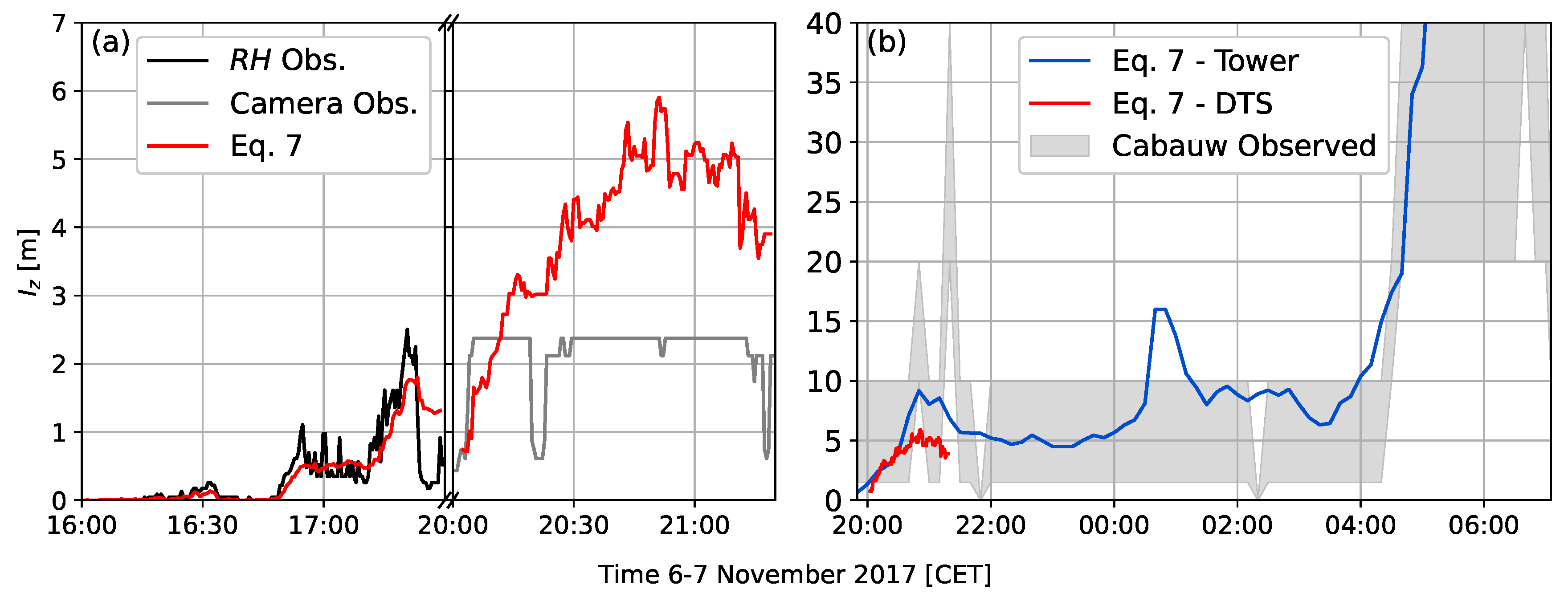
3.2. Comparison with High-Resolution Observations

We estimate q s and q as a function of height from the wet and dry-bulb temperatures. These were then used to calculate Equation (7) and estimate the fog depth as a function of time.
We first look at the so-called “saturation interface”, and not the fog interface itself. Due to microphysical effects these are not necessarily the same. We define the saturation interface as the point at which the DTS observations indicate an RH value of ≥99% (rather than 100%). Figure 5a, left, shows the observed interface depth (back line) and the projected depth (red) of the interface determined with Equation (20), starting at 16.00 local time and calculated every 30 s, as consistent with the observational resolution. We stop the comparison at 17.30, after which freezing of the wet-bulb fiber meant that reliable RH estimates could no longer be calculated. Note that no filtering of either the observed or estimated interfacial depths was performed. The agreement between the observed saturation interface depth and the projected interface is striking. The initial growth of the saturated layer is captured accurately, as are periods of the saturated layer shrinking.
Due to freezing conditions, the value of q cannot be accurately estimated until after the fog layer has deepened above the freezing layer (roughly 20.00 local time). After this point, we diagnose the fog interface from the one-minute camera images. Again, the forward-integrated fog depth (red line, Figure 5a, right) agrees well with the observed depth of the fog layer (gray line), capturing an initial steep growth before eventually exceeding the maximum observable height of the camera (2.5 m). Unfortunately, the accuracy above this height cannot be directly confirmed.

3.3. Comparison with Tower Observations

We also estimate the growth rate of the fog layer using the coarser-resolution tower observations (Figure 5b). Due to the observational resolution of the tower, we can only say that the fog interface exists between the highest level at which visibility is ≤1 km. For example, if visibility is 500 m at 1.5 m height, and 3 km at 10 m height, then the fog interface exists between 1.5 and 10 m height. This is the shaded region in Figure 5b.
The estimated fog depth (blue line) fits extremely well within the constraining envelope, deepening steadily throughout the night, and, other than a temporary deepening event estimated around 01:00, reaching the 10 m and 20 m levels at the correct time. This is particularly encouraging as any errors in the projected fog depth would accumulate over the long period of integration (roughly 10 h). The DTS-estimated fog depth from Figure 5a is also plotted in Figure 5b (red line), showing good agreement between the two estimated depths, in spite of the difference in spatio-temporal resolution of the DTS and tower.
This is, of course, only one event. We did, however, also look at the agreement between observed and estimated fog depths for a further 238 shallow (<40 m) radiation fog events that occurred at the CESAR facility between April 2011 and September 2020 (Figure 6). We compute the deviation of the estimated I z from the observed range. If the estimated depth falls within the envelope, then the deviation is 0; otherwise, the difference is calculated between the estimated fog depth and the nearest range boundary. While there are some instances of very large differences between the observed and estimated I z , the majority agree. In particular, I z falls within the correct range more than 80% of the time within the first 3 h of fog onset, and, except for 5 h and 10 h, is accurate more than 60% of the time.

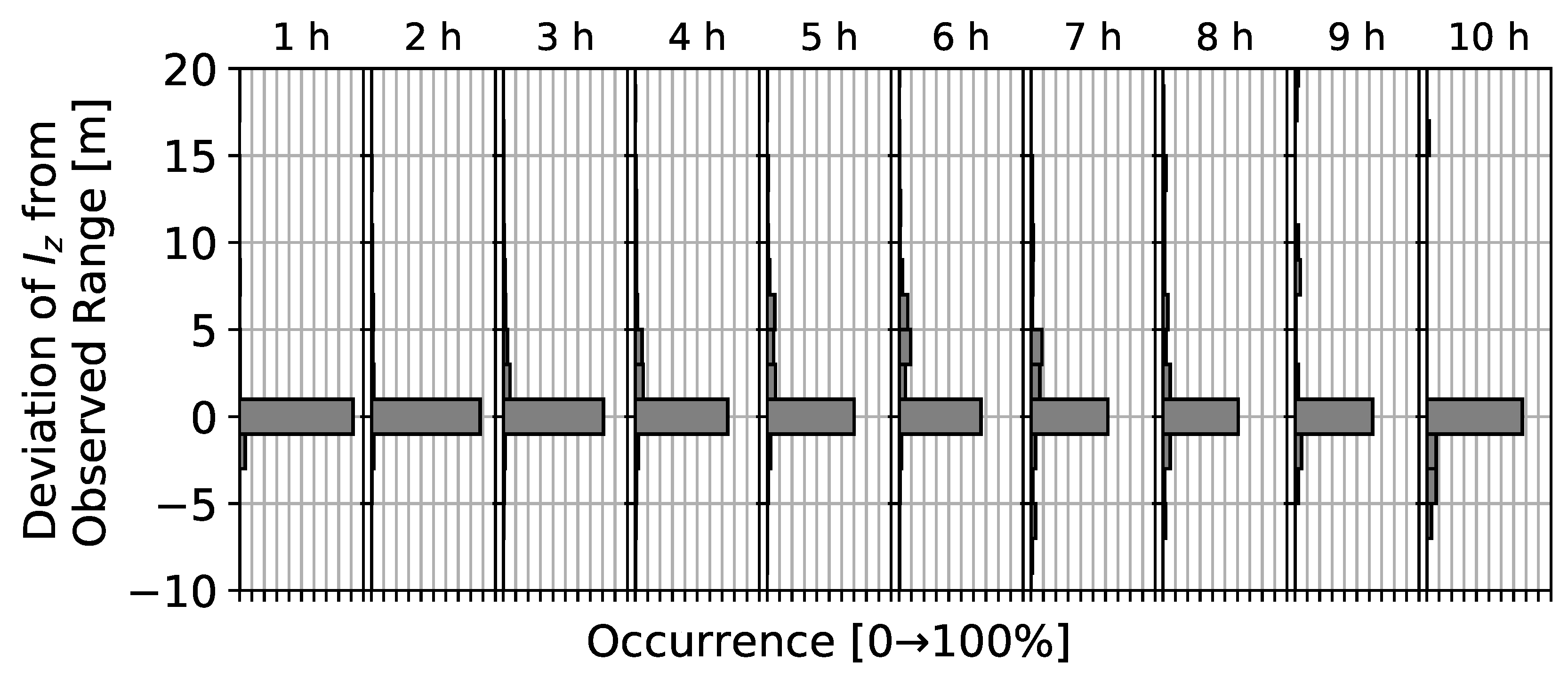
3.4. Errors and Uncertainty

Equation (7) inherits error and uncertainty from the observed specific humidity and temperature. Appendix A presents the mathematical propagation of uncertainty through Equation (7), as well as the implications of assuming a bulk (linearized) vertical derivative.
Using the observation precision at the CESAR facility, we present the uncertainty (random error) in the growth as the possible change in depth over 10 min in Figure A1a ( ± s E 7 Δ t ; Equation (A3)). Compared to the observed fog depth, the uncertainty ranges between approximately 10 and 30% of the estimated fog depth. As the fog deepens, however, the relative uncertainty is reduced. The greatest uncertainties arise when either of the numerator or denominator of Equation (7) approach 0 (no or infinite growth, respectively).
Errors will also arise through the necessary discretization of the vertical gradients. When taking the bulk gradient between two observational heights (i.e., Δ q s / Δ z ), we show (Figure A1b) that the gradient may be significantly underestimated close to the lower bound, and overestimated as the upper bound is approached, increasing almost linearly for a logarithmic profile. This means that the growth may be subsequently overestimated when close to z 1 (denominator too small), and underestimated close to z 2 . As the fog depth increases, the impact of discretization becomes less significant. Overall, discretization results in what is likely a conservative estimate of fog evolution, particularly near the surface, with the fog depth initially estimated to be larger than in reality.

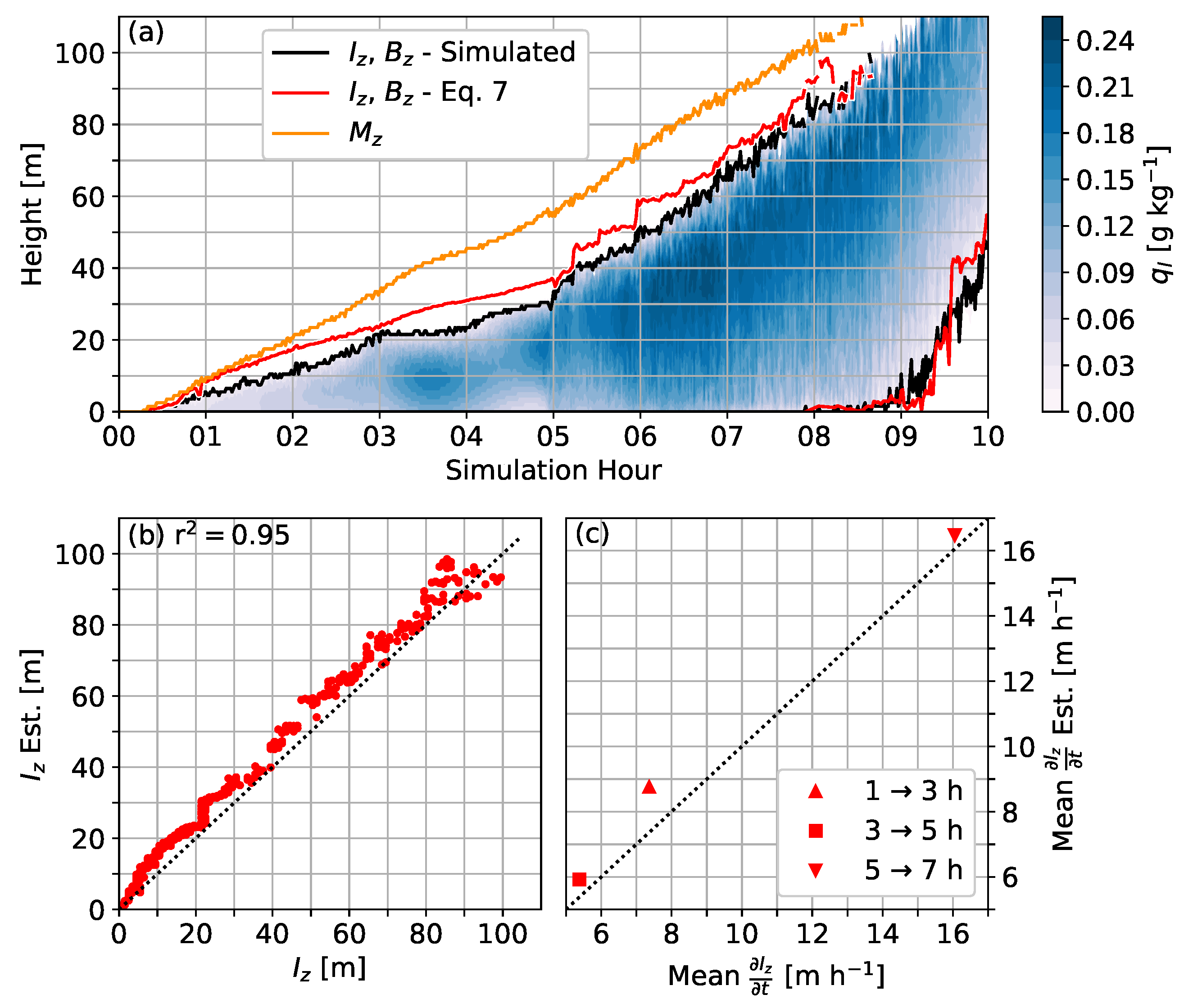
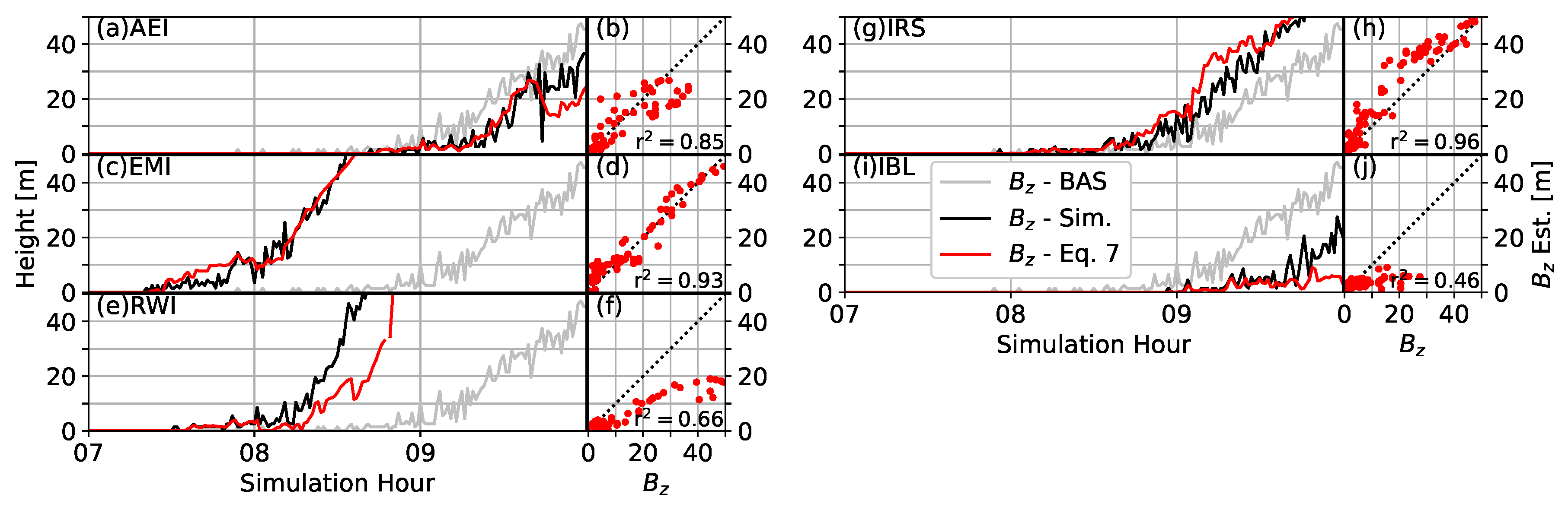
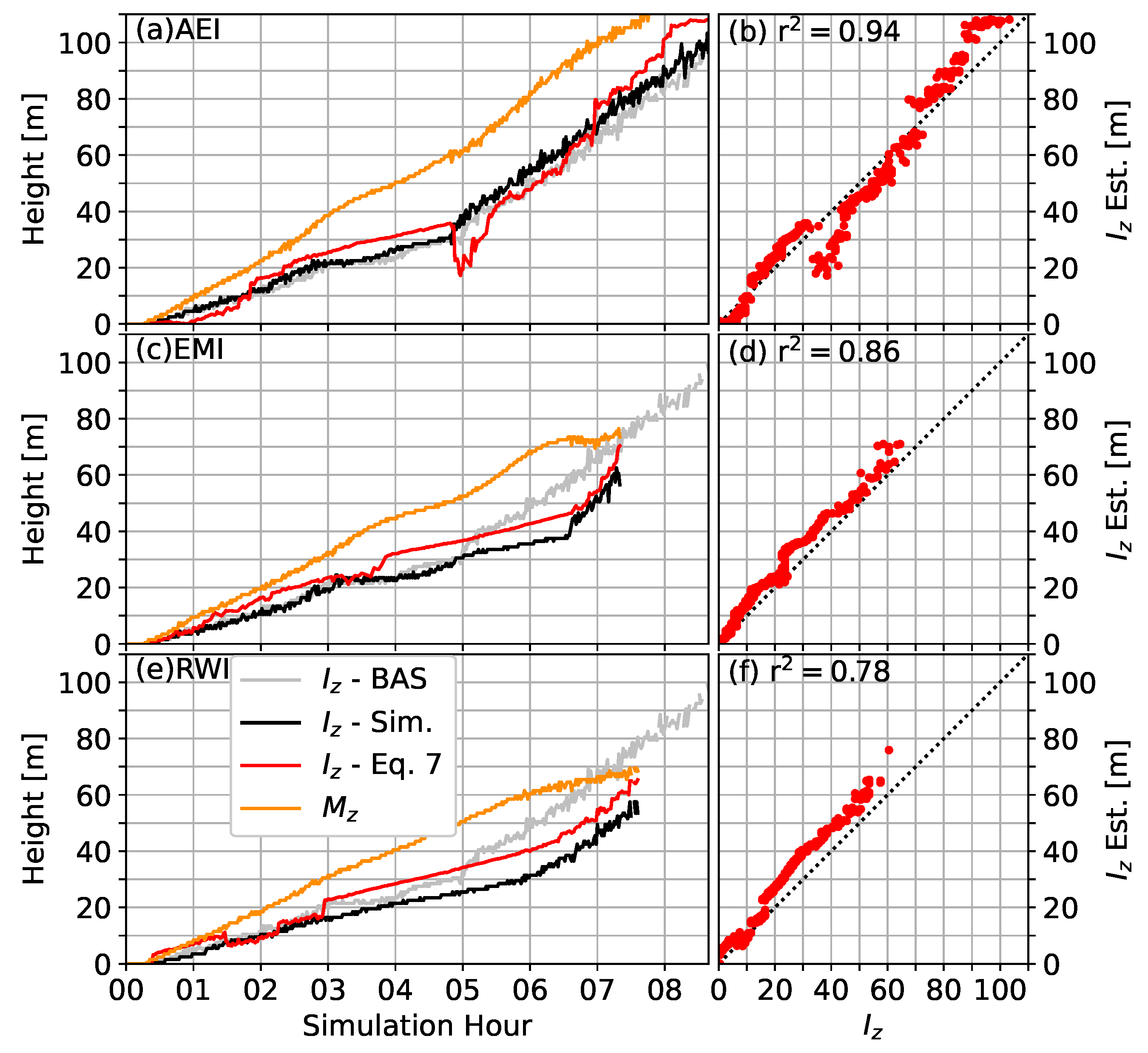
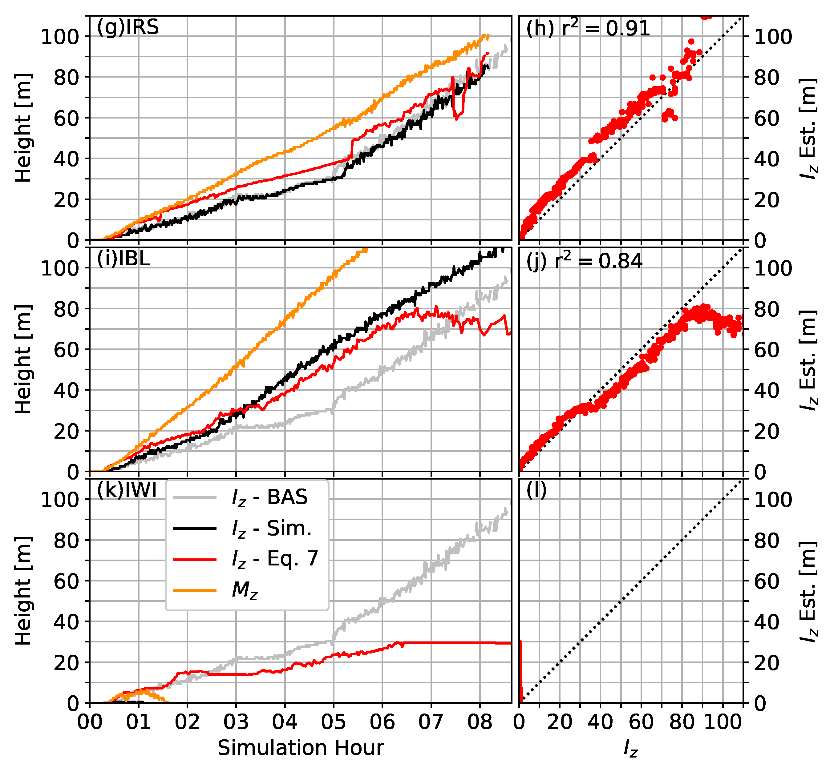
4. Comparison with Large-Eddy Simulation Output
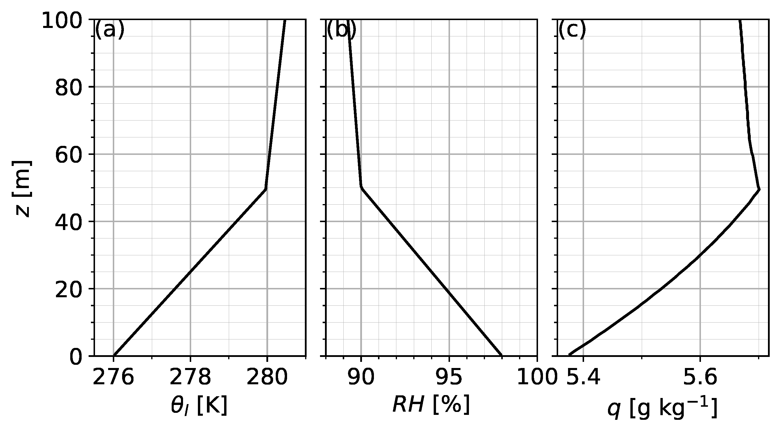
Due to observational—primarily vertical resolution—constraints, we are unable to accurately observe a deep (optically thick) fog layer; above 40 m height on the tower, Δ z becomes >40 m, which does not allow for reliable derivatives to be estimated. Therefore, we also run a series of simple large-eddy simulations (LES) to indicate whether Equation (7) might also hold for deeper (and simulated) fog layers. We use the Dutch Atmospheric Large Eddy Simulation (DALES [13]) for our simulations. DALES is an open source atmospheric model written to simulate a range of processes, including stratocumulus clouds as well as convective and stable boundary layers. It was also previously used to simulate the dissipation of fog [14]. DALES is available at https://github.com/dalesteam/dales. For the purposes of this work, the specific formulation of DALES is not discussed. Instead, the interested reader is directed to [13] for further detail.
It is important to note that in this section we are not so much concerned with the accuracy of the simulation. Instead, it is intended simply as an illustration and test of the qualitative principles behind Equation (7). A more detailed numerical investigation is welcomed in future research.

4.1. Case Setup

The simulated case is based on a fog event observed on 23 March 2011 at the CESAR facility, which was previously simulated [5] and described in the literature [15]. In total, we performed seven simulations (see Table A1 and Table A2), each with a three-letter identifier. The baseline set-up (BAS) most closely resembles the reference set-up in [5].
The simulations are initialized at midnight with idealized profiles as in [5] (Figure A2). Piece-wise linear profiles with a boundary-layer depth of 50 m are defined for the liquid water potential temperature ( θ l ) and relative humidity (RH), which are then used to determine the initial profile of q t according to the DALES formulations. We use a small computational domain, measuring just 50 m × 50 m in the horizontal (representing the same area as the energy-balance field in which the DTS observations in Section 3 were made) and 384 m in the vertical. We recognize that the horizontal extent of the domain is small compared to the ultimate depth of the fog layer and will restrict the scale of the simulated turbulence. However, the early stages of fog development within the stable boundary layer will be represented accurately. Further, initial tests on domain size showed little difference in the overall fog evolution, with the small domain therefore selected as providing a balance between computational efficiency and accuracy. Again, we note that we are also not concerned with producing a 100% accurate simulation of the case as we are with testing the qualitative principles behind the equations presented.
In the lowest 100 m of the domain, a grid cell resolution of 1 m 3 ( Δ x = Δ y = Δ z = 1 m) was used. Above 100 m height, the vertical grid was stretched linearly with a slope of 1.25 m per grid cell (maintaining a 1-m horizontal resolution). Periodic boundary conditions were used in the horizontal direction. The simulation output was time-averaged and saved every minute (of simulated time). Further detail on the case set up and simulation specifications can be found in Appendix B.
We performed six additional simulations with modified parameters compared to BAS (Table A2). Aerosols were increased (AEI) from N c = 150 cm 3 to N c = 200 cm 3 , such that there is a greater number of smaller droplets. Enhanced near-surface mixing (EMI) was achieved through increasing the values of z 0 for momentum and heat by 10%. To modify the amount of mixing due to vertical shear, we perform simulations with a reduced wind speed (RWI) of U g e o = 3 m s 1 , and an increased wind speed (IWI), with U g e o = 5 m s 1 (from 4 m s 1 in the BAS case). Finally, to test the influence of the vertical gradients on growth, the slopes of temperature in the residual layer (IRS) and depth of the boundary layer (IBL) were increased, maintaining the same temperature and RH values at the surface and top of the BL.
We attempted to perform additional simulations beyond the six included here (e.g., modifying the surface conductivity, decreasing the depth of the boundary layer, or with larger changes in the variables); however, due to the challenge of simulating the stable conditions, these additional simulations either produced no fog, or saw complete turbulent collapse that resulted in problems when calculating near-surface thermodynamic variables. As it stands, the only simulation included here that produced no liquid water is IWI; however, it is included for completeness and to provide one example of fog-free conditions.
We determine the simulated saturation interface from profiles of the liquid water specific humidity, q l , at the horizontal center of the domain. Note, we do not take the average over the domain, but the values from the single central column. Averaging would smooth out some of the smaller fluctuations, while the choice of column has little influence on the result. We choose to use the LES results, rather than performing single column model simulations, as LES does not rely on turbulent parametrizations, which can struggle to capture the transition between stable, weakly stable, and neutral conditions that occur during the fog lifecycle. We use a threshold value of q l 0.01 g m 3 (same as in [5]) to identify the foggy/saturated layer. I z is only determined when the saturated layer is in contact with the surface (i.e., before lifting after sunrise). We then determine I z / t as the discrete derivative of the simulated I z in time. As with the observational comparison in Section 3, we also estimate the gradients at the interface and use them to project the growth rate forward in time from t = 0 to estimate I z (Equation (20)). Given the numerical setting, we are also able to determine the position of the lower interface after lifting ( B z ), and diagnose its position and lifting rate according to the same process as I z . We further estimate the value of M z using an iterative approach as described in Section 2.2, and assuming a liquid water content of 0.15 g m 3 for a fog layer [16]. Where a mixed value of 0.15 g m 3 or greater cannot be achieved, even for the existing saturated layer, M z is set to the value of I z .

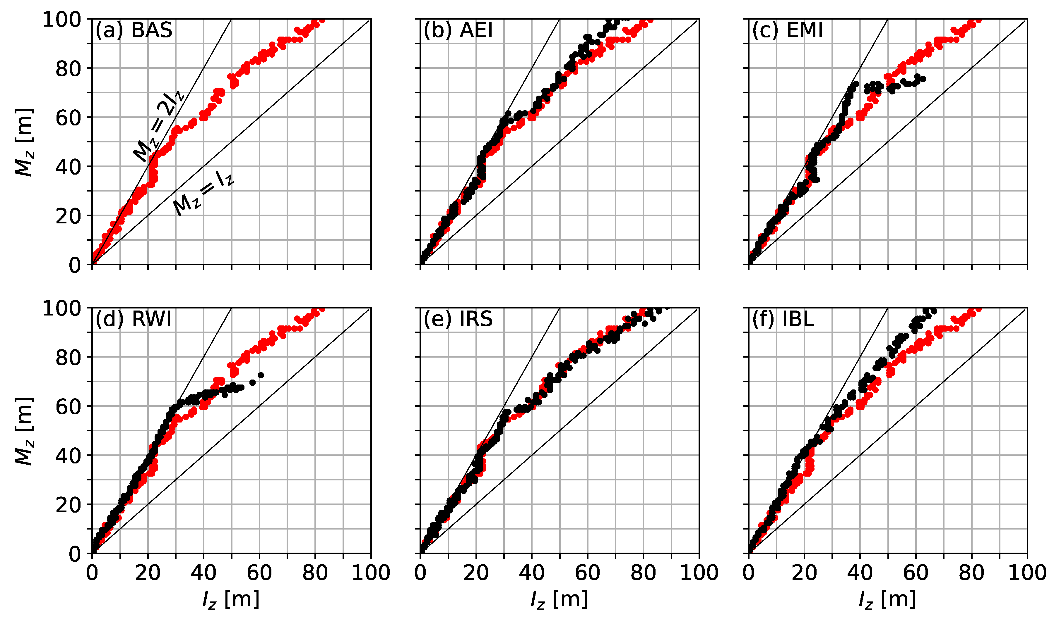
4.2. Simulation Results

We present the results of the BAS simulation in Figure 7. One-minute profiles of q l are shown in Figure 7a, along with the diagnosed and projected upper and lower interfaces, I z and B z , as well as the estimated MAMD. Figure 7b,c shows the direct comparison between the estimated and simulated I z , and mean growth rates, respectively. We determined the mean rates as the average over the two-hour periods indicated. Overall, the estimated interface agrees very well (r 2 = 0.95 ) with the simulated interface, even over the roughly nine hours of estimation. I z is slightly overestimated, but that is primarily due to just a few points where the growth rate is too high. Notably, the average growth rates during the 2 h periods are very similar.
The estimated and simulated interface heights of the other simulations from Table A2 are shown in Figure A3. As with BAS, I z is well-estimated using the analytical expression in Equation (7), and projected forward in time as in Equation (20). Although the depth is different than the BAS case, the simulated and estimated interfaces agree well (r 2 = 0.78 0.94 ). As with the BAS simulation, the value of I z approaches M z toward the end of the simulation.
In Figure 8, M z is plotted as a function of the simulated I z for all fog-forming simulations. M z remains around 2 I z for all simulations while up to I z 25 m (approximately 2–5 h into the simulations). This identifies the transition from an optically thin, stably stratified fog layer to an optically thick, well-mixed fog layer. As the level of mixing increases, M z and I z converge. During the transition period, M z continues to deepen while I z remains nearly constant. This is because the fog layer continues to cool, with the restricted vertical growth leading to a build-up of excess moisture in the fog layer.
Figure 7 and Figure 9 also plot the simulated and estimated values of the lower interface, B z , after the fog lifts from the ground, becoming a shallow stratocumulus cloud. As with the upper interface, the lifting of the cloud base is also well described by Equation (7). The agreement between simulated and estimated B z is particularly good for BAS, AEI, EMI, and IRS (r 2 = 0.85 0.96 ), even with large variations in the lifting rate between the simulations. Overall, B z is underestimated for the RWI and IBL simulations, though still qualitatively similar. Due to the lack of liquid water simulated in IWI, B z is irrelevant.
The IBL and IRS cases (Figure A3g,i) demonstrate the importance of the vertical gradients in determining the growth rate. With the deeper BL (IBL), the slope in temperature is correspondingly shallower in order to maintain the same temperature at BL-top. As a result, due to the reduced stability near the surface and the smaller denominator in Equation (7), the fog layer grows much more rapidly. M z is also much deeper for the IBL simulation as the profile is such that more of the layer is near saturation (reduced slope). At the same time, the “stalling” seen in other simulations does not occur. Instead the fog layer is able to grow continuously throughout its evolution. Conversely, the increased slope in the residual layer (IRS), though only a difference of 10%, is enough to slow the growth rate slightly compared to the BAS simulation.
The analysis in Section 2.1.2 (Equation (11)) suggests that the growth rate of radiation fog increases with time, due to the fact that the strongest inversion occurs close to the surface. Interestingly, this appears to be a general feature of the fog growth in our simulations (see, e.g., in Figure 7c), due to the smaller vertical gradient above the BL. One also sees that the growth temporarily slows during transition from optically thin to optically thick fog (approximately between 3 to 5 h), though this may also be related to the boundary-layer height of the simulation. During this time, there is an overestimation of I z , which is primarily due to an initial overestimation at the time of the vertical profiles becoming well-mixed (top-down convection). After this initial overestimation in the interface depth ( I z / t too large as the denominator is close to 0), the mean estimated and simulated growth rates are approximately equal (e.g., Figure 7c).

5. Summary and Discussion

We begin by first summarizing the previous sections, followed by a discussion of the utility and significance of the results presented herein.
In Section 2, we derive an analytical expression to describe the rate of deepening/erosion of a fog interface. Given the conditions under which fog exists, the relative moistening or drying at the interface determines whether the fog layer will deepen or erode, while the gradients in specific and saturation-specific humidities modulate the rate of growth. We also present a lengthscale estimate of the maximum depth that a fog layer can achieve, the maximum attainable mixed depth (MAMD), as might occur if there was a sudden mixing event that equalizes the vertical profiles of temperature and humidity. This MAMD gives an indication of the robustness of a fog layer to a given level of mixing; any mixing deeper than MAMD, or a reduction in MAMD below the existing fog depth, will lead to dissipation of some or all of the fog. The ratio of MAMD to I z is therefore important in assessing the persistence of a fog layer in its current state.
We subsequently validate the analytical formulation in Equation (7). We utilized both a high-resolution and a coarse-resolution data set for the observational comparison (Section 3). In both cases, the analytical expression results in an estimated fog depth that agrees very well with the observed fog interface, lending confidence to its accuracy. Even with the coarser data from the CESAR tower, the timing of deepening is remarkable, especially considering the length of the night over which the estimated interface is determined. This is not only true for the highlighted case, but also for 238 events assessed between April 2011 and September 2020. Unfortunately, though, the observational data are insufficient for a truly direct comparison. First, the coarse resolution (especially from the tower data) means that only an approximate agreement can be determined. Second, observations of deeper fog layers are needed to ensure the relationship holds for optically thick fog layers; the resolution above 40 m height (at least at the CESAR facility) is too coarse to determine reliable vertical gradients.
Instead, we performed several simple numerical simulations of an idealized radiation fog layer, in order to generate a surrogate dataset to further illustrate the analytical principles (Section 4). While the simulations are simple in nature, they are still able to provide insight into the qualitative behavior of the fog layer, which can be related back to Equation (7). The estimated interface depths again agree very well with the simulated depths; both for the baseline (BAS) case, and the perturbed cases (see Table A2). Problems mainly arise when the denominator of Equation (7) is close to zero (very shallow vertical gradients), in which case very large values of I z / t are estimated. This means that either shorter integration times need to be used, or such spikes must be removed or averaged in order to obtain accurate estimates of I z .
In addition to the estimated interface depth, we also determine M z for the simulations, assuming a well-mixed fog layer. Throughout the first few hours, M z remains at the expected 2 I z for all simulations (Figure 8), with the two values approaching each other after the transition. The more rapid deepening of M z than I z in the middle of the simulations is likely due to the restriction of vertical mixing as the top of the boundary layer is reached, and the time of transition from optically thin to optically thick fog. During this time, I z is mechanically constrained, while the super saturation continues to increase significantly due to the continued cooling within the shallow layer.
Of the seven simulations that we performed, only the one with increased geostrophic wind speed (IWI) resulted in no simulated fog (Figure A3k), with dew point only briefly achieved at the surface near the beginning of the simulation. However, applying Equation (7) would still lead to an estimated fog layer that is 30 m deep. This highlights the need to ensure that Equation (7) be applied to estimate the growth of an existing fog layer, rather than to forecast a fog layer that has not yet appeared. Otherwise, the assumptions and the conditions in Section 2 are not met, and the relationship is invalid.

5.1. Equation (7) to Interpret the Evolution of Typical Fog Layer

We now highlight how Equation (7) can be used to interpret and understand the evolution of a fog layer. The observations in Section 3.2 and simulations in Section 4 indicate that such a fog layer will initially grow slowly, with accelerating growth before slowing toward the transition to well-mixed fog. Eventually, top-down erosion of the fog interface, or lifting of the cloud at the surface will take place.
We begin by assuming a very shallow radiation fog forming within a quasi-steady, stable boundary layer. The fog will grow according to the rate of quasi-steady cooling (Equation (9)). Due to the decreasing vertical gradients (smaller denominator) with height, the rate of growth increases with fog depth (Equation (11)). The acceleration means that there is a sort of “early warning” in the system (such as highlighted in [2]). At the same time, Equation (7) also implies that there is a maximum growth rate possible for a given temperature profile (Equation (12)).
As the fog layer undergoes the transition to a well-mixed fog layer, the gradients in temperature and moisture become smaller below the interface, and larger above the interface. According to the analysis here, this results in a slowing of the fog growth (see, e.g., Figure A3), with competing profiles above and below the interface; the more uniform profile just below the interface favours erosion of the fog layer. A similar “upside-down” interface exists when the fog lifts from the surface, becoming a shallow stratocumulus cloud. As with the fog top, this lower interface is also seen to be well-described by the analytical expression that we derive in Section 2, as evidenced through the numerical comparison in Figure 7 and Figure 9. The well-mixed profile means that just a small amount of warming or drying is needed in order to reduce the relative humidity at the surface.
Under stable conditions, M z is shown to be approximately equal to 2 I z (Section 2.2.1). This means, intuitively, that deeper fog layers are more robust to increases in turbulent mixing, whereas shallow fog layers can be rapidly dissipated. This is evidenced in the “twin nights” presented in Figure 8 of [17], where an increased wind speed on the second night prevents a fog layer from forming, in spite of otherwise identical conditions. Significant deviation from the 2:1 ratio indicates that mixing has taken place (Figure 8). The closer I z is to M z , the more mixing has occurred, but also the closer the fog layer is to its maximum sustainable depth. Beyond a height of M z , the fog layer cannot be sustained unless significant moistening occurs. This leads to the fog-top erosion, or cloud-base lifting seen toward the end of a fog’s lifecycle, which, as above, can be understood through the small denominator of Equation (7).

5.2. Equation (7) as a Diagnostic Tool

Beyond simply understanding, our analytical expression enables the estimation of fog depth, particularly in settings where discrete observational levels are insufficient for continuous tracking of fog depth. Equation (7) provides this, with the time and space derivatives able to be determined from previous observations, and used to project the evolution forward in time (e.g., Equation (20)). This can be used as both an a priori estimate of fog evolution in the coming minutes or hour, as well as an a posteriori tool for tracking the evolution of a fog layer, and relating it to the processes involved. It may also be that the methodology is useful in a numerical setting, providing a sub-grid indication of fog depth.
Equation (7) also provides a means of determining the sensitivity of fog layer to calculation errors, as well as to changes in physical processes. In particular, when the denominator of Equation (7)—which modulates the growth rate—is small, the fog layer will be extremely sensitive to any changes in moisture, e.g., through advection or changes in turbulent mixing. This carries over into the computational domain, where numerical experiments will become increasingly sensitive to slight computation or input errors.
All of this assumes that the gradients and time derivatives can be accurately determined. Within the near-saturated SBL, errors in determining temperature and humidity can be large. We provide a means of estimating the uncertainty in Equation (7) in Appendix A. The uncertainty ranges between 10 and 30% of the estimated depth resulting when projected over the 10-min integration period (Figure A1a). Note, this analysis is only relevant for the CESAR facility, and will vary with differences in instrument precision and placement at different sites. It is important to recognize that this represents the range of uncertainty in the estimates, but not necessarily the error in the fog depth. It does not take into account the challenge, for example, of estimating q at high relative humidities, which will manifest as a bias or offset. That being said, the magnitude of vertical gradients in q s is typically much larger than that of q, particularly near the surface in the stable boundary layer, therefore the vertical gradient of q in particular is less important. A consistent bias will not appear in the time derivative as it cancels out when the difference is taken.
Estimating the vertical gradients using the discrete observations will also have an impact on the accuracy of the results. For example, under (very) stable conditions, q s / z can be underestimated when close to the lower observation level, and overestimated as the second level is approached (Figure A1b). This means that while the mean growth rate can be determined, shallower fog may be estimated to grow more rapidly than in reality, and deeper for more slowly. To account for this, it may make sense to take the average derivative over two neighboring depth ranges, rather than assume the bulk. This will be much closer to the true derivative at that location. One could alternatively assume an analytical fit to the temperature profile as done in Appendix A; however, this is not guaranteed to be representative of the actual conditions.
The true error will depend on the exact nature of the evolution, including the compensation, compounding, and counteraction of different errors. Ultimately, the smooth prediction of depth as opposed to a highly variable estimate), suggests that possible errors may result from systematic bias but not from random errors. Even still, the evolution of our estimated fog depth agrees well with the observed evolution, suggesting that if there is an error due to a bias in the observations, it does not significantly affect our estimates over short periods of time. It is likely, however, that the increased deviation of the estimated I z after approximately 4 h (Figure 6) is due to the compounding of errors in earlier stages.
The above is important to remember when applying any of the equations presented herein. However, the observational and numerical comparisons do still suggest the method is reliable, even under challenging conditions. Equation (7) also provides us with a means of understanding the sensitivity of our observations/predictions to errors. By including approximate errors into the framework, we see how sensitive results may be. For example, if the error means that the sign of Equation (7) changes, then the conditions are extremely sensitive to miscalculation. On the other hand, it may be that the overall magnitude of the terms is sufficiently large that the errors only affect the magnitude, but not the actual growth/erosion.

5.3. Specific Processes at the Interface

Price and Stokkereit [18] have shown through the use of infrared imagery that several processes can influence the evolution of a fog layer. It is beyond the scope of this research to explicitly consider the specific processes that modify the terms in Equation (7), however one could utilize the conceptual framework here in addition to leveraging multiple sources of information in order to interpret the evolution. For example, the moisture budgets could be determined through consideration of relevant boundary layer processes, rather than observational diagnosis alone. Ultimately, relevant processes can be broadly grouped into three categories: radiative, advective, and turbulent processes. While the exact role of any process will depend on the specific conditions, we briefly discuss them here.
Radiative cooling will serve to modify the saturation specific humidity through means of altering the temperature in both time and space. As the fog layer becomes optically thick, the cooling interface will change, sharpening vertical temperature gradients near fog top (slowing the growth of fog), while at the same time, continuing to cool the interface (leading to fog deepening). In the absence of other processes, the growth rate will remain positive, but gradually decrease in time.
Advection of cooler and or more moist air will lead to a deepening of the fog layer; often a rapid deepening as the vertical gradients are reduced. Conversely, warmer, drier air will lead to evaporation and dissipation of the fog. The ultimate state of saturation will depend on the amount of mixing that takes place, and the original state of the air masses in question [6,19].
It has been shown that turbulence acts to limit the formation of radiation fog, with weak to no wind required (see, e.g., in [20]). At the same time, others have found that at least some turbulence is necessary for fog formation in order to mix the air vertically and lead to saturation over a deeper region (see, e.g., in [21]). In [6], a threshold is defined for the level of turbulence ( w 2 < 0.002–0.005 m 2 s 2 ) for radiation fog to form, provided the air is sufficiently close to saturation; above this threshold, the air will dry out, rather than lead to a saturated mixture. We can further reconcile the role of turbulence through contemplation of Equation (7) as follows. Turbulent mixing will serve to reduce the vertical gradients of temperature and humidity, such that the denominator becomes smaller, increasing sensitivity of the fog top to changes in moisture. At the same time, however, turbulent transport will also (under stable conditions) bring warmer, (relatively) drier air from aloft, and reduce the relative moistening at the interface. If the turbulent mixing is too great, then erosion will take place. In the case of weak to no turbulence, a quasi-steady boundary layer will form, where the gradients remain approximately constant. This means that any growth will be driven by the relative moistening through cooling by radiative processes alone, which is a much slower process. We see this reflected even in our simple simulations. The fog layer grows deeper and more rapidly in our BAS simulation than either of the reduced or increased wind cases (RWI and IWI). In the case of the former, this may be due to the reduced vertical mixing, while in the latter no fog forms due to the too-large drying influence.

6. Conclusions

We derive an analytical expression that expresses the rate of fog deepening or erosion as the ratio of the time derivatives of moisture to the vertical gradients (Equation (7)):
I z t = q t q s t q s z q z 1 .
The denominator is always positive in the case of fog top, and the sign of the numerator governs whether the fog layer will deepen or erode. Observations and simple simulations of idealized fog layers show that the relationship does a good job of explaining the fog evolution.
We also present a lengthscale estimate of a fog layer: the maximum attainable mixed depth (MAMD). This is both an indication of the depth a fog layer could potentially reach due to a sudden mixing event, as well as the maximum depth over which mixing can occur before a fog layer will dissipate due to insufficient moisture content. Under stable conditions, we show this to be approximately 2 I z ; significant deviation from this ratio indicates that mixing has occurred and that the fog layer may be closer to dissipation.
The analytical description can be applied diagnostically. It is particularly useful for identifying the growth rate and interface depth in an observational setting. Where observations are limited to discrete heights, Equation (7) can be used to identify the position of the fog interface between levels. This can then be related back to observed processes, and possibly used to improve the output of numerical models by providing a more precise location of fog height, rather than simply an observed range of possible depths. Further, it may prove useful as a subgrid component of numerical models, though that is not directly investigated here.
The analytical framework also provides a formalized means of understanding why fog evolves the way it does. Through consideration of the equation and the contributing processes, one can identify the role that different factors play in the growth and dissipation of a fog layer. Among other things, we show that acceleration of fog growth with height, the temporary pause in growth during the transition to well-mixed fog, and the ultimate dissipation and/or lifting can all be explained through Equation (7) and the concept of the MAMD.
We recognize that the present analysis is very much of local nature, and primarily focused on radiation fog. It would be interesting, however, to extend the present rationale to advective tendencies as well in order to obtain a more general description of fog growth and erosion. It would also be enlightening to assess the full budget equations for the upper interface—including turbulent mixing processes, radiative cooling, and advective tendencies—in order to quantify the gradients and tendencies in Equation (7). This would be particularly interesting in conjunction with the use of a range of data sources, including traditional sensors and emerging techniques such as infrared photography. A more extensive numerical study to investigate the results in greater detail would be welcomed as an important follow up. Finally, we welcome further testing of the presented metrics in a range of settings, including, other observational sites, as well as numerical weather prediction.

Author Contributions

Conceptualization, formal analysis, writing—review and editing, and project administration: J.G.I. and B.J.H.v.d.W.; methodology, investigation, validation, visualization, and writing—original draft preparation, J.G.I.; supervision and funding acquisition, B.J.H.v.d.W. All authors have read and agreed to the published version of the manuscript.

Funding

This research was funded by European Research Council Consolidator Grant number 648666. The APC was funded by the Delft University of Technology Library.

Acknowledgments

We thank Steven van der Linden and Antoon van Hooft for their contributions during discussions throughout the preparation of this work. We are also grateful to Stephan de Roode and Maurice van Tiggelen for their assistance with DALES, as well as Peter Baas for his input in the early stages of the research. Finally, we thank the three anonymous reviewers and the editors for their valuable feedback throughout the review process. The DTS data can be obtained via the 4TU data repository [12], and the KNMI data is available from the KNMI data centre: https://data.knmi.nl/datasets?q=CESAR. DALES is an open-source model available at https://github.com/dalesteam/dales.

Conflicts of Interest

The authors declare no conflict of interest. The funders had no role in the design of the study; in the collection, analyses, or interpretation of data; in the writing of the manuscript; or in the decision to publish the results.

Appendix A. Estimating Errors and Uncertainties

Appendix A.1. Propagation of Uncertainties

We use the linear error propagation formula (see, e.g., in [22]) in order to provide an estimate of the uncertainty of Equation (7) due to uncertainty in the observed meteorological values. For any dependent variable, y, with n independent variables x 1 , x 2 , up to x n , the uncertainty in y ( s y ) depends on the squared sum of the errors/uncertainties in x n ( s n ), multiplied by the derivatives of y with respect to x n :
s y 2 = s x 1 2 y x 1 2 + s x 2 2 y x 2 2 + + s x n 2 y x n 2 + 2 s x 1 , x 2 y x 1 y x 2 + 2 s x i , x j y x i y x j
The cross terms account for any correlation between the errors in the independent variables x n , with s x i , x j = ρ x i , j s x i s x j , and ρ x i , x j the correlation between the errors for all i j in n. Using the error propagation formula, the uncertainty in Equation (7) can be expressed as
s E 7 2 = s q z 2 E 7 q z 2 + s q t 2 E 7 q t 2 + s q s , z 2 E 7 q s , z 2 + s q s , t 2 E 7 q s , t 2
We write I z / t as simply E 7 , and the time and space derivatives using the subscripts t and z, respectively, in order to improve the readability of the equations. We assume, for simplicity, that there is no correlation between errors in q and q s . Assuming discretized derivatives, we arrive at the following equation for the uncertainty,
s E 7 2 = 2 β 2 E 7 Δ z 2 + 1 Δ t 2 s q 2 + s T 2 q s T 2 .
At the CESAR facility, the air and dewpoint temperatures are recorded with a precision of 0.1 K [23], which results in a precision of ~0.7% in the value of specific humidity. The resulting uncertainty—indicative of the random error introduced in an observation—is half of this value (i.e., s T = ± 0.05 K and s q = 7 q / 2000 ). Using these values in the uncertainty analysis, we estimate the uncertainty in the projected depth over 10 min as ± s E 7 Δ t , with the results shown Figure A1 for the observation period in Figure 5b.
The temperature sensors are also calibrated to an accuracy of 0.1 K under ideal conditions. Further systematic errors are possible during conditions of low wind speed and high humidity, such as during foggy conditions. These systematic errors are difficult to quantify, though will manifest in the observations as a consistent offset or bias. The impact of radiation, which can lead to significantly elevated temperatures, is not relevant during nocturnal conditions.
Figure A1. (a) Estimated uncertainty in the projected growth of fog for the CESAR observations presented in Figure 5b based on instrument precision. (b) Ratio of discrete to exact vertical gradient of q s assuming a logarithmic temperature profile, and over the first three depth ranges at CESAR.
Atmosphere 11 00865 g0a1

Appendix A.2. Error Due to Discrete Vertical Gradients

In order to take the vertical derivatives, we assume that the gradients in q and q s can be well approximated as the simple linear difference between two vertical levels. In the stable boundary layer, however, the profile of temperature is distinctly nonlinear, which will influence the vertical derivative of the saturation specific humidity. To illustrate this, we can assume that the temperature can be expressed with logarithmic form,
T ( z ) = T 0 + m ln z z 0 and T ( z ) z = m z
where m is the slope and T 0 is the temperature at height z 0 . Using the chain rule, the vertical gradient of the saturation specific humidity is
q s ( z ) z = q s , 0 exp A T ( z ) 273.15 T ( z ) B A 273.15 B T ( z ) B 2 m z .
The corresponding discretized (mean) derivative, where z 1 < z < z 2 , is
Δ q s Δ z = q s , 2 q s , 1 z 2 z 1 = q s , 0 exp A T 2 273.15 T 2 B exp A T 1 273.15 T 1 B z 2 z 1 .
such that the ratio of the linearized derivative to the true derivative is
Δ q s Δ z q s z 1 = z m α Δ z z 2 z ζ 2 z 1 z ζ 2
where
α = A 273.15 B T 2 + m ln z z 2 B 2 and ζ n = A m 273.15 B T n B T n m ln z z n B
Figure A1b shows the ratio for the observed ranges at Cabauw, up to an observation height of 40 m. Close to z 1 , the derivative is significantly underestimated, while it is overestimated as I z approaches z 2 .

Appendix B. Additional Information Regarding the Large-Eddy Simulations

In this appendix, we present additional information, including tables and figures, in support of Section 4. Table A1 and Table A2 present an overview of the parameters used in the BAS and modified simulations, respectively.
Table A1. Overview of the main parameters used to initialize the BAS simulation. Parameters modified for the other simulations are listed in Table A2.
SymbolParameterValue
λ Surface conductivity4 W K 1  m 2
N c Droplet number concentration150 cm 3
s T , BL Slope of temperature in the BL0.08 K m 1
s T , RL Slope of temperature in the RL0.01 K m 1
RH 0 Surface relative humidity98%
RH BL Relative humidity at BL top90%
RH TOP Relative humidity at top of domain85%
T 0 Surface temperature276 K
T S Soil temperature279 K
U g e o Geostrophic wind speed4 m s 1
z m a x Maximum height of domain384 m
z BL Depth of the initial boundary layer50 m
z 0 , m Roughness length for momentum0.15 m
z 0 , h Roughness length for heat0.235 × 10 4  m
Table A2. Overview of the six additional simulations performed, with the the remaining parameters the same as in the BAS set-up (Table A1).
SimulationChanged Parameters
AEIAerosols increased N c = 200  cm 3
EMIEnhanced mixing z 0 , m = 0.165  m, z 0 , h = 0.259 × 10 4  m
RWIReduced geostrophic wind speed U g e o = 3  m s 1
IWIIncreased geostrophic wind speed U g e o = 5  m s 1
IRSIncreased residual slope s T , RL = 0.011  K m 1
IBLBL-depth increased s T , BL = 0.04  K m 1 , z BL = 100  m
Figure A2 shows the initial profiles of θ l , RH, and q used to initialize the BAS simulation. Within a boundary layer of 50 m depth, θ l increases linearly from 276 K with a slope of 0.08 K m 1 , while RH decreases from 98% in the lowest grid cell to 95% at the top of the boundary layer (BL). Above the BL, θ l increases more slowly at 0.01 K m 1 , and RH goes from 90% to 85% at the top of the domain.
Within the model, radiative transfer is calculated via the rapid radiative transfer model developed for general circulation models (RRTM-G, [24]), as well as the bulk microphysical scheme of [25,26], with droplet settling enabled. Note that initial tests showed little dependence on the microphysical scheme employed. The surface is described by an interactive scheme with four soil layers (of uniform temperature).
Figure A2. Initial profiles, as described in [5] of (a) temperature, (b) relative humidity, and (c) specific humidity (calculated from T and RH) for the BAS simulation.
Atmosphere 11 00865 g0a2
Figure A3 plots the comparison for the additional simulations presented in (Table A2). In the left-hand column, we show simulated I z , along with the estimated value of I z using Equation (7), and M z . For comparison, I z from the BAS simulation is shown in gray. On the right, the estimated I z is compared directly with the simulated I z . Except for the IWI simulation where no fog formed, I z is very well estimated with Equation (7).
Figure A3. Estimated and simulated interface heights for the simulations in Table A2. (a,c,e,g,i,k) Time series of estimated and simulated fog depth, including the simulated depth from the BAS simulation (as in Figure 7a). (b,d,f,h,j,l) 1:1 comparison of estimated fog depth to simulated fog depth (as in Figure 7b).
Atmosphere 11 00865 g0a3aAtmosphere 11 00865 g0a3b

References

  1. Smith, D.K.E.; Renfrew, I.A.; Price, J.D.; Dorling, S.R. Numerical Modelling of the Evolution of the Boundary Layer during a Radiation Fog Event. Weather 2018, 73, 310–316. [Google Scholar] [CrossRef] [Green Version]
  2. Izett, J.G.; Schilperoort, B.; Coenders-Gerrits, M.; Baas, P.; Bosveld, F.C.; van de Wiel, B.J.H. Missed Fog? On the Potential of Obtaining Observations at Increased Resolution during Shallow Fog Events. Bound. Layer Meteorol. 2019. [Google Scholar] [CrossRef] [PubMed] [Green Version]
  3. Román-Cascón, C.; Yagüe, C.; Steeneveld, G.J.; Sastre, M.; Arrillaga, J.A.; Maqueda, G. Estimating Fog-Top Height through near-Surface Micrometeorological Measurements. Atmos. Res. 2016, 170, 76–86. [Google Scholar] [CrossRef] [Green Version]
  4. Ju, T.; Wu, B.; Zhang, H.; Liu, J. Parameterization of Radiation Fog-Top Height and Methods Evaluation in Tianjin. Atmosphere 2020, 11, 480. [Google Scholar] [CrossRef]
  5. Maronga, B.; Bosveld, F.C. Key Parameters for the Life Cycle of Nocturnal Radiation Fog: A Comprehensive Large-Eddy Simulation Study. Q. J. R. Meteorol. Soc. 2017, 143, 2463–2480. [Google Scholar] [CrossRef]
  6. Price, J.D. On the Formation and Development of Radiation Fog: An Observational Study. Bound.-Layer Meteorol. 2019, 172, 167–197. [Google Scholar] [CrossRef]
  7. Moene, A.F.; van Dam, J.C. Transport in the Atmosphere-Vegetation-Soil Continuum; Cambridge University Press: New York, NY, USA, 2014. [Google Scholar]
  8. Dyer, A.J. A Review of Flux-Profile Relationships. Bound.-Layer Meteorol. 1974, 7, 363–372. [Google Scholar] [CrossRef]
  9. Penman, H.L. Natural Evaporation from Open Water, Bare Soil and Grass. Proc. R. Soc. Lond. Ser. A Math. Phys. Sci. 1948, 193, 120–145. [Google Scholar]
  10. Monna, W.; Bosveld, F. In Higher Spheres: 40 Years of Observations at the Cabauw Site; Koninklijk Nederlands Meteorologisch Instituut: De Bilt, The Netherlands, 2013; Volume 232. [Google Scholar]
  11. Selker, J.S.; Thévanez, L.; Huwald, H.; Mallet, A.; Luxemburg, W.; de Giesen, N.V.; Stejskal, M.; Zeman, J.; Westhoff, M.; Parlange, M.B. Distributed Fiber-Optic Temperature Sensing for Hydrologic Systems. Water Resour. Res. 2006, 42, W12202. [Google Scholar] [CrossRef] [Green Version]
  12. Izett, J.G.; Schilperoort, B.; Coenders-Gerrits, M.; van de Wiel, B.J.H. High-Resolution DTS Temperature Measurements during Fog at Cabauw. Dataset 2018. [Google Scholar] [CrossRef]
  13. Heus, T.; van Heerwaarden, C.C.; Jonker, H.J.J.; Siebesma, A.P.; Axelsen, S.; van den Dries, K.; Geoffroy, O.; Moene, A.F.; Pino, D.; de Roode, S.R.; et al. Formulation of the Dutch Atmospheric Large-Eddy Simulation (DALES) and Overview of Its Applications. Geosci. Model Dev. 2010, 3, 415–444. [Google Scholar] [CrossRef] [Green Version]
  14. Wærsted, E.G.; Haeffelin, M.; Steeneveld, G.J.; Dupont, J.C. Understanding the Dissipation of Continental Fog by Analysing the LWP Budget Using Idealized LES and in Situ Observations. Q. J. R. Meteorol. Soc. 2019, 145, 784–804. [Google Scholar] [CrossRef]
  15. Boers, R.; Klein Baltink, H.; Hemmink, H.J.; Bosveld, F.C.; Moerman, M. Ground-Based Observations and Modeling of the Visibility and Radar Reflectivity in a Radiation Fog Layer. J. Atmos. Ocean. Technol. 2013, 30, 288–300. [Google Scholar] [CrossRef]
  16. Pilie, R.; Eadie, W.; Mack, E.; Rogers, C.; Kochmond, W. Project Fog Drops Part I: Investigations of Warm Fog Properties; Contractor Report CR-2078; National Aeronautics and Space Administration (NASA): Washington, DC, USA, 1972.
  17. Izett, J.G.; van de Wiel, B.J.H.; Baas, P.; Bosveld, F.C. Understanding and Reducing False Alarms in Observational Fog Prediction. Bound. Layer Meteorol. 2018, 169, 347–372. [Google Scholar] [CrossRef] [Green Version]
  18. Price, J.; Stokkereit, K. The Use of Thermal Infra-Red Imagery to Elucidate the Dynamics and Processes Occurring in Fog. Atmosphere 2020, 11, 240. [Google Scholar] [CrossRef] [Green Version]
  19. Taylor, G.I. The Formation of Fog and Mist. Q. J. R. Meteorol. Soc. 1917, 43, 241–268. [Google Scholar] [CrossRef]
  20. Roach, W.T.; Brown, R.; Caughey, S.J.; Garland, J.A.; Readings, C.J. The Physics of Radiation Fog: I-a Field Study. Q. J. R. Meteorol. Soc. 1976, 102, 313–333. [Google Scholar] [CrossRef]
  21. Duynkerke, P.G. Turbulence, Radiation, and Fog in Dutch Stable Boundary Layers. Bound.-Layer Meteorol. 1999, 90, 447–477. [Google Scholar] [CrossRef]
  22. Bevington, P.R.; Robinson, D.K. Data Reduction and Error Analysis for the Physical Sciences, 3rd ed.; McGraw-Hill: Boston, MA, USA, 2003. [Google Scholar]
  23. Bosveld, F.C. Cabauw In-Situ Observational Program 2000–Now: Instruments, Calibrations and Set-Up. 2019. Available online: http://projects.knmi.nl/cabauw/insitu/observations/documentation (accessed on 14 August 2020).
  24. Mlawer, E.J.; Taubman, S.J.; Brown, P.D.; Iacono, M.J.; Clough, S.A. Radiative Transfer for Inhomogeneous Atmospheres: RRTM, a Validated Correlated-k Model for the Longwave. J. Geophys. Res. Atmos. 1997, 102, 16663–16682. [Google Scholar] [CrossRef] [Green Version]
  25. Seifert, A.; Beheng, K.D. A Double-Moment Parameterization for Simulating Autoconversion, Accretion and Selfcollection. Atmos. Res. 2001, 59–60, 265–281. [Google Scholar] [CrossRef]
  26. Seifert, A.; Beheng, K.D. A Two-Moment Cloud Microphysics Parameterization for Mixed-Phase Clouds. Part 1: Model Description. Meteorol. Atmos. Phys. 2006, 92, 45–66. [Google Scholar] [CrossRef]
Figure 1. (a) Sketch of the conditions in which fog exists, following Equation (4). Given the hypothetical profile of q s near the interface, the profile of q must exist within the shaded regions, represented by the dashed line. (b) Equation (7) illustrated as a ladder against a wall. The shallower (steeper) the ladder, the lesser (greater) the distance that can be travelled vertically.
Atmosphere 11 00865 g001
Figure 2. Fog growth in a quasi-steady stable boundary layer. (a) The rate of growth as in Equation (11). (b) The value of I z in time. The dashed lines indicate the linear growth rate at I z = 3 L / α and the maximum growth rate.
Atmosphere 11 00865 g002
Figure 3. Illustration of M z using linear temperature and relative humidity profiles. M z is deeper than I z due to the super saturation within the fog layer. In stable conditions, M z 2 I z (Section 2.2.1).
Atmosphere 11 00865 g003
Figure 4. M z and I z as a function of slope for a linear temperature profile with T 0 = 275 K and two values of q ¯ , corresponding to relative humidities at the surface of 102% and 110%, respectively. M z is determined iteratively as well as using the approximate solution in Equation (19). Note that in both cases, M z 2 I z .
Atmosphere 11 00865 g004
Figure 5. Observed fog height compared with the height estimated by forward integration of Equation (7). (a) High-resolution comparison using distributed temperature sensing (DTS)-estimated saturation (i.e., RH = 99 % as the interface (left) and the camera-derived observations of fog depth. (b) Comparison against the fog depth observed along the Cabauw tower. Note, the camera is limited to a depth of 2.25 m, and the tower is restricted to discrete heights such that the observed fog depth is between the maximum height of observed fog, and the level above.
Atmosphere 11 00865 g005
Figure 6. Deviation of estimated I z from the observed range for 238 shallow radiation fog events observed at the CESAR facility between April 2011 and September 2020. The PDFsshow the difference in 2 m bins, over each hour after fog onset.
Atmosphere 11 00865 g006
Figure 7. Baseline (BAS) simulation. (a) Liquid water specific humidity with lines indicating the simulated and estimated (according to Equation (20)) I z , B z , and M z . (b) 1:1 comparison of estimated fog depth to simulated fog depth. (c) Comparison of mean estimated growth rate (Equation (7)) with simulated growth rate over two-hour segments.
Atmosphere 11 00865 g007
Figure 8. M z vs. I z for the simulations, with M z = 2 I z and M z = 2 I z for comparison. (a) BAS simulation. (bf) Labelled simulation (black) on top of BAS simulation (red).
Atmosphere 11 00865 g008
Figure 9. The simulated and estimated locations of the lower interface, B z , for each of the six simulations in Table A2. (a,c,e,g,i) Time series of estimated and simulated B z compared to B z from the BAS simulation (Figure 7a). (b,d,f,h,j) 1:1 comparison of estimated B z to simulated B z (as in Figure 7b).
Atmosphere 11 00865 g009

