Article

Light Scattering in a Turbulent Cloud: Simulations to Explore Cloud-Chamber Experiments

1
Department of Physics and Atmospheric Sciences Program, Michigan Technological University, 1400 Townsend Dr., Houghton, MI 49931, USA
2
Department of Physics and Astronomy, College of Charleston, 66 George St., Charleston, SC 29424, USA
*
Author to whom correspondence should be addressed.
Atmosphere 2020, 11(8), 837; https://doi.org/10.3390/atmos11080837
Submission received: 24 June 2020 / Revised: 31 July 2020 / Accepted: 3 August 2020 / Published: 7 August 2020
(This article belongs to the Special Issue The Motion of Particles in Turbulence)

Abstract

:
Radiative transfer through clouds can be impacted by variations in particle number size distribution, but also in particle spatial distribution. Due to turbulent mixing and inertial effects, spatial correlations often exist, even on scales reaching the cloud droplet separation distance. The resulting clusters and voids within the droplet field can lead to deviations from exponential extinction. Prior work has numerically investigated these departures from exponential attenuation in absorptive and scattering media; this work takes a step towards determining the feasibility of detecting departures from exponential behavior due to spatial correlation in turbulent clouds generated in a laboratory setting. Large Eddy Simulation (LES) is used to mimic turbulent mixing clouds generated in a laboratory convection cloud chamber. Light propagation through the resulting polydisperse and spatially correlated particle fields is explored via Monte Carlo ray tracing simulations. The key finding is that both mean radiative flux and standard deviation about the mean differ when correlations exist, suggesting that an experiment using a laboratory convection cloud chamber could be designed to investigate non-exponential behavior. Total forward flux is largely unchanged (due to scattering being highly forward-dominant for the size parameters considered), allowing it to be used for conditional sampling based on optical thickness. Direct and diffuse forward flux means are modified by approximately one standard deviation. Standard deviations of diffuse forward and backward fluxes are strongly enhanced, suggesting that fluctuations in the scattered light are a more sensitive metric to consider. The results also suggest the possibility that measurements of radiative transfer could be used to infer the strength and scales of correlations in a turbulent cloud, indicating entrainment and mixing effects.

1. Introduction

Radiative transfer is different in a cloud in which droplet positions are spatially correlated than in a homogeneous cloud with the same mean properties such as droplet size and number density. How to quantitatively describe the changes in radiative transfer under conditions where the scale of the correlations is smaller than the mean free path and where the medium must be considered discrete rather than continuous, such as in atmospheric clouds, remains an open question [1,2,3]. Qualitatively, this is due to the presence of voids and clusters, where photons propagate further in dilute regions and experience stronger extinction in more dense regions [4]. Properly predicting radiative transfer through inhomogeneous media has many applications, including the cloudy atmosphere [5,6], where pockets of clear and cloudy air on multiple spatial scales can be formed by mixing and entrainment [7,8]. The majority of work focusing on radiative transfer through correlated media has been theoretical and computational in nature [9,10,11], at least in part due to the difficulty of such measurements. For example, in recent published work [12], we numerically examined various aspects of radiative transfer through idealized homogeneous and clustered monodisperse particle distributions of discrete particles. We found that while direct transmission is increased in the presence of spatial correlation, diffuse forward transmission is reduced by a similar amount (nearly offsetting the increase in direct transmission). In Packard et al. [12], the particle clustering was idealized in order to give clear results; the purpose of this paper is to take a step toward experimental verification by exploring computationally whether deviations from standard radiative transfer for a homogeneous medium can plausibly be detected in a laboratory-generated cloud containing more realistic spatial correlations in droplet position due to turbulent mixing.
We consider polydisperse distributions of discrete particles within a turbulent cloud generated in a laboratory convection cloud chamber as our motivating context. We address the problem of predicting radiative transfer through both homogeneous and inhomogeneous media using a Monte Carlo Ray Tracing (MCRT) methodology previously shown [12] to be consistent with standard radiative transfer [13]. To limit scope, we focus this work on the transmission of visible light (e.g., nominal wavelength 550 nm) through an atmospheric cloud generated under laboratory conditions. In the visible spectrum and for the water droplet sizes considered here (large compared to the wavelength), Mie theory indicates that absorption is practically nonexistent. Consequently, in this study, we assume a single scatter albedo of unity.
Our principal motivation is the use of simulation to explore experimental designs for measuring the existence and magnitude of deviations from standard radiative transfer due to particle clustering in a laboratory cloud chamber such as the Pi convection cloud chamber, which is able to produce long-lasting (statistically stationary) mixing clouds [14]. Specifically, we consider what measurable quantities would be most beneficial for a study of the influence of spatial correlations. In a previous publication [12], we focused on monodisperse distributions with somewhat extreme Matérn clustering and optical thickness near unity; a single particle size and rather small, dense collections of droplets were used for much of our analysis as we evaluated the role of radial distribution functions. In this work, a primary interest is the extent of deviation from the spatially homogeneous case expected when more realistic (as generated by turbulent convection) spatial correlations, smaller optical thicknesses, and polydisperse size distributions are present.
The optical thicknesses we consider, near 0.1, were chosen to mimic the experimental conditions feasible under dynamical equilibrium within the Pi Chamber (e.g., mixing clouds). Larger optical depths can be simulated but are harder to achieve in an experimentally controllable context. The choice of total optical thickness also focuses on a regime where multiple scattering is not dominant.
To represent radiative transfer in a real system, such as the Pi convection cloud chamber, we consider a medium consisting of air and discrete droplets dispersed within a confined geometry. Computer simulation, acting as a surrogate laboratory, allows for the prediction of experimental results and the development of an effective methodology for measuring relevant parameters without complicating factors such as imperfect instrumentation.
In this work, a Large Eddy Simulation (LES) code is used to generate clouds with properties (such as optical thickness, particle size distribution function, and spatial correlation) realistic for a laboratory-generated mixing cloud in the Pi Chamber [15]. A MCRT code, capable of simulating scattering events with appropriate phase functions, propagates individual photons from a normally incident collimated beam through the LES-generated particle distribution, while tracking direct, diffuse forward and diffuse backward radiative fluxes. Two types of spatial particle distributions were employed, the first using the droplet locations exported from the LES, and the second replacing these particle locations with uniformly random positions to remove any spatial correlation. Hereafter, the product from the former method will be referred to as “LES-positioned”, since the particle locations come directly from LES exports; the latter method will be referenced as “random” or “homogeneous” due to the lack of spatial correlation. Directional radiative transfer components (e.g., direct, diffuse forward, backward and total forward flux) are compared to determine the impact of realistic spatial correlation in a hypothetical laboratory setting.
The paper proceeds as follows: First, we briefly describe the MCRT scattering code and its ability to employ particle distributions imported from LES cloud realizations. Next, we describe the LES methodology and summarize some of the most relevant statistics of the numerous cloud samples extracted for the scattering simulations. Then, we present results of the simulations, showing the impact of spatial correlations on direct and diffuse radiative fluxes. The analysis is focused on changes in both mean and fluctuations of optical fluxes. In the discussion section, we discuss the results and their implications for potential cloud radiative transfer measurements in a laboratory setting.

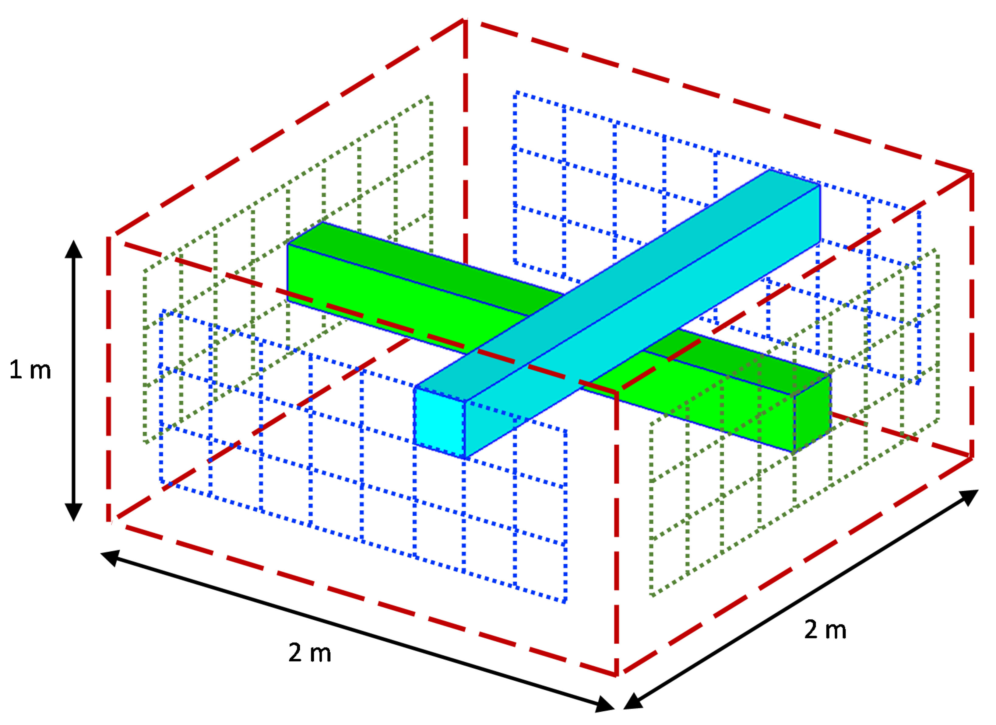
2. Simulated Experiments

2.1. Summary of the Monte Carlo Ray Tracing (MCRT) Methodology

2.1.1. Overview of the MCRT Code (‘mcScatter’)

The Monte Carlo scattering software used for our analysis, referred to as ‘mcScatter’, is a ballistic photon simulation code [10,16] created to explore radiative transfer through scattering media, such as light transport through an atmospheric cloud [12]. The construction of this Monte Carlo Ray Tracing (MCRT) code was motivated, in part, by a desire to eventually compare numerical results with experiments performed in a laboratory cloud chamber [14]. The mcScatter software is summarized here for convenience; a more detailed description can be found in [12] and its supplemental material.
The MCRT code allows users to specify particle size, optical wavelength, complex index of refraction (to model various types of droplets and wavelengths), as well as boundary conditions for the computational domain. Here, we focus our analysis on visible wavelengths (e.g., 550 nm) and examine chamber-realistic cloud droplet sizes based on previous laboratory measurements [14,17]. The resulting size parameters concentrate our analysis on the single-scattering, forward-scattering dominant regime with a single scatter albedo of unity and a scattering efficiency of Qsca ≈ 2. Motivated by a realistic optical path through the Pi Cloud Chamber described in [7], the virtual spatial domain is limited to 2 m along the propagation distance. The cross section of the domain is taken as 0.2 × 0.2 m, as in [12], chosen as a compromise between computational efficiency and allowing lateral diffusion of scattered light in predominantly single-scatter media.
Monte Carlo numerical methods [18,19,20,21] employ large numbers of random draws to explore problems for which closed-form solutions may not exist, such as propagation through heterogeneous media [4,22,23]. Photons are virtually cast into a medium, scattering events are detected, and new scattering angles are chosen using a Mie or Henyey–Greenstein [24,25,26] scattering phase function. This process is repeated until all rays exit the medium. Many Monte Carlo numerical methods avoid assigning physical locations to particles; instead, the distribution of free paths between consecutive scattering interactions is modeled stochastically via random draws from an analytic cumulative density function (CDF) based on the concentration of particles in the medium [13]. Conversely, in a ballistic ‘photon’ simulation [10,16], particles in a volume are placed at specific locations [27,28]. By employing an explicit location for each particle in the medium, geometric ray-tracing can be used to explore any spatial distribution, including the possibility of particle size-dependent correlations, since scattering events are determined by the intersection between a photon ray’s path and a particle (i.e., a geometric “collision”). Since ballistic photon simulation allows for particle spatial distributions of any kind, there is no need to assume a stochastic free path distribution model.
Other methods, such as approaches derived directly from Maxwell’s equations [29,30], incorporate a detailed electromagnetic treatment of the problem and are especially well-suited for continuous media. However, even for a small atmospheric cloud (e.g., many millions of particles) with varying particle radii, methods like the superposition T matrix remain largely impractical [29] and justify the use of alternative approaches. Ballistic photon simulations, in contrast, are well-matched for resolving generalized spatially correlated media [16]. Our ray tracing Monte Carlo radiative transfer approach is consistent with standard radiative transfer theory [13] and is a computationally feasible method for exploring various heterogeneous media.
During a mcScatter simulation, ray segments are traced through particle fields, accounting for scattering events. Direct and diffuse flux components, both backward and forward, are recorded at numerous physical depths in the virtual cloud. This allows for the calculation of direct, diffuse forward, backward, and total forward irradiance components as a function of physical depth in the cloud with far more three-dimensional detail than can be achieved with any physical measurement, but of course, with the disadvantage that the technique is so computationally expensive that only a small number of samples can be considered; this is exacerbated if specific angles need to be considered, whereas in an experiment under statistically stationary conditions, there is considerable freedom in angular placement of detectors and extent of data collection. Additionally, of course, the experiment includes all relevant physics, whereas the Monte Carlo ray approach depends on the idealizations of the ray tracing method. Further details regarding the implementation of the scattering code and comparisons with theoretical and other published numerical works can be found in Packard et al. [12].

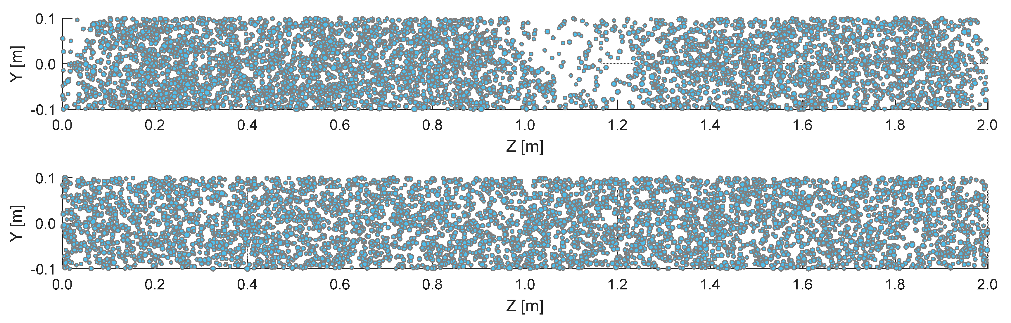
2.1.2. Use of the ‘mcScatter’ MCRT Software with Chamber-Realistic Particle Distributions

The MCRT software mcScatter can perform ballistic photon scattering simulations using a variety of virtual atmospheric media, including both monodisperse and polydisperse particle size distributions with either homogeneous or spatially correlated spatial distributions. In our most recent publication [12], we focused on the impact of spatial correlation on depth-dependent direct and diffuse radiative transfer for monodisperse particle distributions. The spatial correlations in that study were generated via Matérn Point Processes, which generate spatially correlated droplet distributions with user-specified parameters [31,32,33].
For the current study, we incorporate the additional but realistic and physically unavoidable complexity of polydisperse particle size distributions found in actual atmospheric conditions, and we simultaneously explore the impact of realistic spatial correlation with the structure expected in a laboratory cloud chamber facility [14]. Computer simulations, referred to as Large Eddy Simulations (LES) and described in Section 2.2, were used to generate realistic particle size and spatial distributions; the output from these simulations was used as an input to the mcScatter photon simulation (rather than employing either homogeneous or idealized Matérn-clustered clouds). Data files generated by the cloud chamber simulations include both the radius of each droplet (quantized to a finite number of size bins) and three-dimensional position of each droplet.
These data files were read by the mcScatter software for analysis, which has the ability to use or ignore the correlated particle locations from the LES-exported records. When the LES-positioned droplet locations are ignored, uniformly random (x, y, z) values are generated for ballistic photon simulation. This allows us to compare realistic polydisperse particle clouds with either homogeneous or realistically correlated spatial properties.

2.2. Large Eddy Simulation

2.2.1. Large Eddy Simulation Methodology

The System for Atmospheric Modeling, referred to as SAM [34], is a Large Eddy Simulation (LES) code modified to simulate the Pi Cloud Chamber [14]. For simulating the aerosol–cloud interactions, the code has been coupled with HUJISBM, a spectral bin microphysics code [35]. To simulate the cloudy Rayleigh–Bénard convection within the Pi Chamber, SAM has been scaled down and the top and lateral boundary conditions have been modified and quantitatively verified against experiments [15]. For completeness, a brief description of the SAM model is provided below.
The dimensions of the simulated cloud chamber are 2 × 2 × 1 m, with the shortest dimension being the height of the volume. We discretized this volume into small cubic boxes of side length 3.125 cm, yielding 64 × 64 × 32 grid boxes. The time step was chosen to be 0.02 s, and the system was initialized with an unstable temperature and water vapor gradient along the direction of gravity. For the current study, we allowed the system to evolve and reach a steady supersaturation of 2.5%, measured as a planar average at the mean height in the chamber (excluding the grid points nearest the chamber sidewalls). Once the steady state supersaturation was reached [15], we injected cloud condensation nuclei (CCN) at the center of the chamber at a rate of 92,400 particles per cm3 per second; all introduced CCN had a radius of 62.5 nm, representing a unimodal CCN distribution at the center of a bin ranging from 56 to 71 nm. The cloud reaches a steady state by striking a balance between activation and removal due to sedimentation. On reaching steady state after 1 h, the system is allowed to persist for another 45 simulated minutes.
Turbulence in the chamber involves multiple timescales, ranging from very fast processes (e.g., dissipation on the order of 0.1 s) to slow processes like large scale oscillations estimated at 90 to 135 s [36]. The 3D particle fields are output every five minutes (at least two times longer than the largest time scale in the system) during this final 45 min evolution to obtain statistically independent droplet distributions within the simulated cloud chamber. Each of the 131,072 grid boxes (3.125 cm on each side) contains a number of droplets which are sorted into 33 different size bins according to their radii. Since the spatial distribution of droplets within each grid box is not resolved, the current study assumes non-intersecting droplets which are randomly distributed within the corresponding grid box volume. To achieve this, the droplets in each of the 3.125 cm cubic grid boxes are redistributed randomly inside its volume; care is taken to avoid droplet intersection while retaining a lack of other correlations on sub-3.125 cm scales.
For analysis purposes, and to be consistent with the MCRT domain, we extracted many subvolumes from the overall chamber volume, each with dimensions of 0.2 × 0.2 × 2.0 m. These rectangular prisms serve as virtual cloud subsamples, through which we can trace many optical paths. To this end, we define a number of rectangular prisms, each of which comprise 3136 adjacent 3.125 cm grid boxes—7 wide, 7 tall, and 64 in the direction of intended photon propagation. Each of these cloud subsamples has dimensions of 21.875 × 21.875 × 200 cm, which is trimmed slightly to the desired 0.08 m3 volume. To improve our statistics, we chose 24 such subvolumes along each of the two perpendicular lateral walls, resulting in a total of 48 cloud subsamples per cloud realization (see Figure 1). Thus, the output from the LES code is a file with a record entry containing an (x, y, z) position and binned radius for each droplet, which serves as the input for our ray tracing Monte Carlo simulation code. Note that, as shown in Figure 1, no cloud subsamples are extracted from regions directly adjacent to a bounding surface of the LES volume.

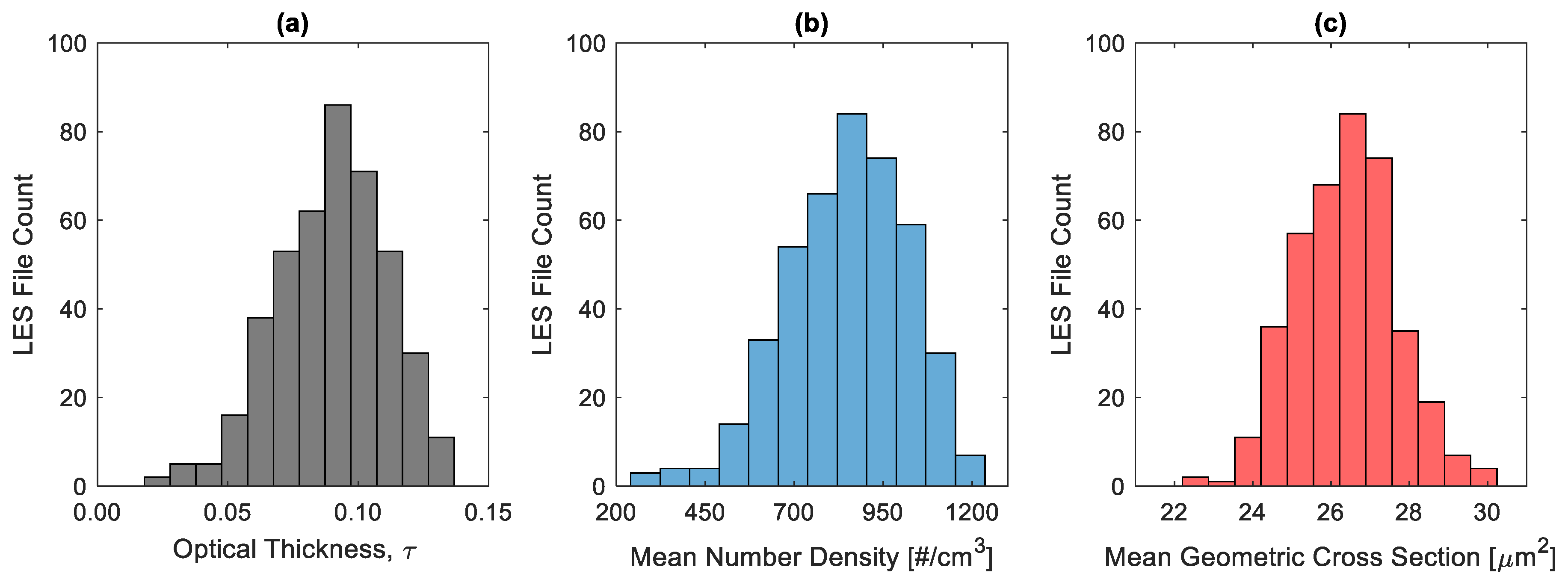
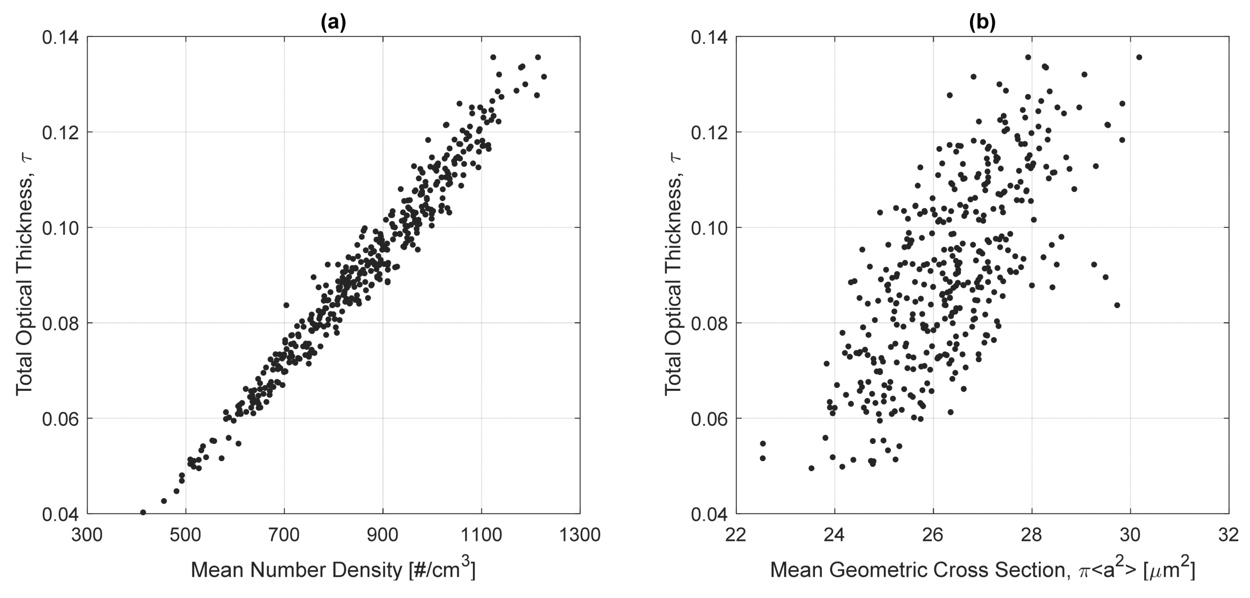
2.2.2. Cloud Microphysical and Optical Properties from the LES

As previously described, after the LES simulation reaches steady state, the system is allowed to evolve for another 45 min and droplet sizes and 3D spatial positions are output from the cloud realization every five minutes for a total of nine statistically independent droplet fields [37,38]. As shown in Figure 1, 48 cloud subsamples are extracted from each of the 9 cloud realizations for a total of 432 cloud subsamples. Before analyzing these cloud subsamples to determine the impact of spatial correlation between droplet positions, we first describe the statistics of their microphysical and optical properties, including mean number density, mean geometric cross section, and total optical thickness. The variation of these properties over the 432 cloud subsamples is shown in Figure 2, with histograms of total optical thickness, number density, and geometric cross section shown in the left (a), center (b), and right (c) panels, respectively.
Here, it is useful to explain that in this work, total optical thickness refers to the total expected optical thickness, based on the assumption of a uniform spatial distribution of particles. This is computed by summing (for all particle radii r) the scattering cross sections of all particles in the distribution ( Q s c a π r 2 ) , scaled by the number density ( N ( r ) / V , where N(r) is the number of scatterers of size r and V is the simulated volume) for each particle size, and multiplying by the propagation distance z along the optical axis:
τ e x p = r N ( r ) V Q s c a π r 2 z .
For simplicity, and to keep the focus of the study on spatial correlations, in the estimate of total optical thickness, the scattering efficiency used in the summation is computed using the geometric approximation (i.e., Qsca = 2). All references to optical thickness in this work refer to expected optical thickness, calculated from particle size distribution functions only, without the use of a scattering simulation to determine computed optical thickness.
Mean number density and total optical thickness are highly correlated (R2 = 0.97), as shown in panel (a) of Figure 3, while mean geometric cross section and total optical thickness are only weakly correlated (R2 = 0.49), as can be seen in the wider spread of points in panel (b) of Figure 3. The strong correlation of optical thickness and mean number density is reminiscent of the expected behavior of a cloud undergoing inhomogeneous mixing: in that case, variations in liquid water content are driven by variations in droplet number density, with droplet diameter remaining constant. Indeed, this type of behavior in the Pi Chamber has been noted in previous work [39]. Similar behavior can be observed in precipitation: the variance of the drop size distribution (or its moments like rainfall rate) can be primarily driven by either the number of drops or by the underlying variability in the size distribution shape, and the dependence even varies with scale [40].
It is worth noting that the chosen approach of large eddy simulation captures the large-scale variability in scalar fields due to anisotropic forcing in Rayleigh–Bénard convection. The variability captured by the LES is consistent with observations in the Pi Chamber [15]. Because the dissipation scales are not resolved, other clustering effects, such as those due to droplet inertia, are not represented. In the context of the Pi Chamber experiments, however, the degree of inertial clustering is extremely small because the turbulence energy dissipation rates are modest, similar to those existing in stratocumulus clouds, and the droplet sizes considered here are small. Specifically, the mean dissipation rate in the bulk fluid is 0.0014 W/kg and for the mean droplet diameter of 5.8 µm, the Stokes number is 1.1 × 10 3 , a factor of 10 below the range where clustering just becomes detectable in most experiments [41]. Furthermore, clustering is further reduced in the low Stokes number regime when gravitational sedimentation is accounted for, and when a broad droplet size distribution exists [42,43]. In conditions where inertial clustering is strong, the radiative effects can be significant [44]. The LES approach taken here will capture the dominant clustering in the cloud chamber experiments due to large-scale scalar mixing effects, and it will be of interest in future work to analyze the additional influence of inertial clustering. In any case, the effects are expected to be independent and consequently, the variance from these sources will be additive. This suggests that the results presented here correspond to a lower bound; if differences between the LES and homogeneous simulated clouds appear potentially measurable in this context, then experimental detection of the differences when inertial clustering is present should give an even stronger signal.

3. Results

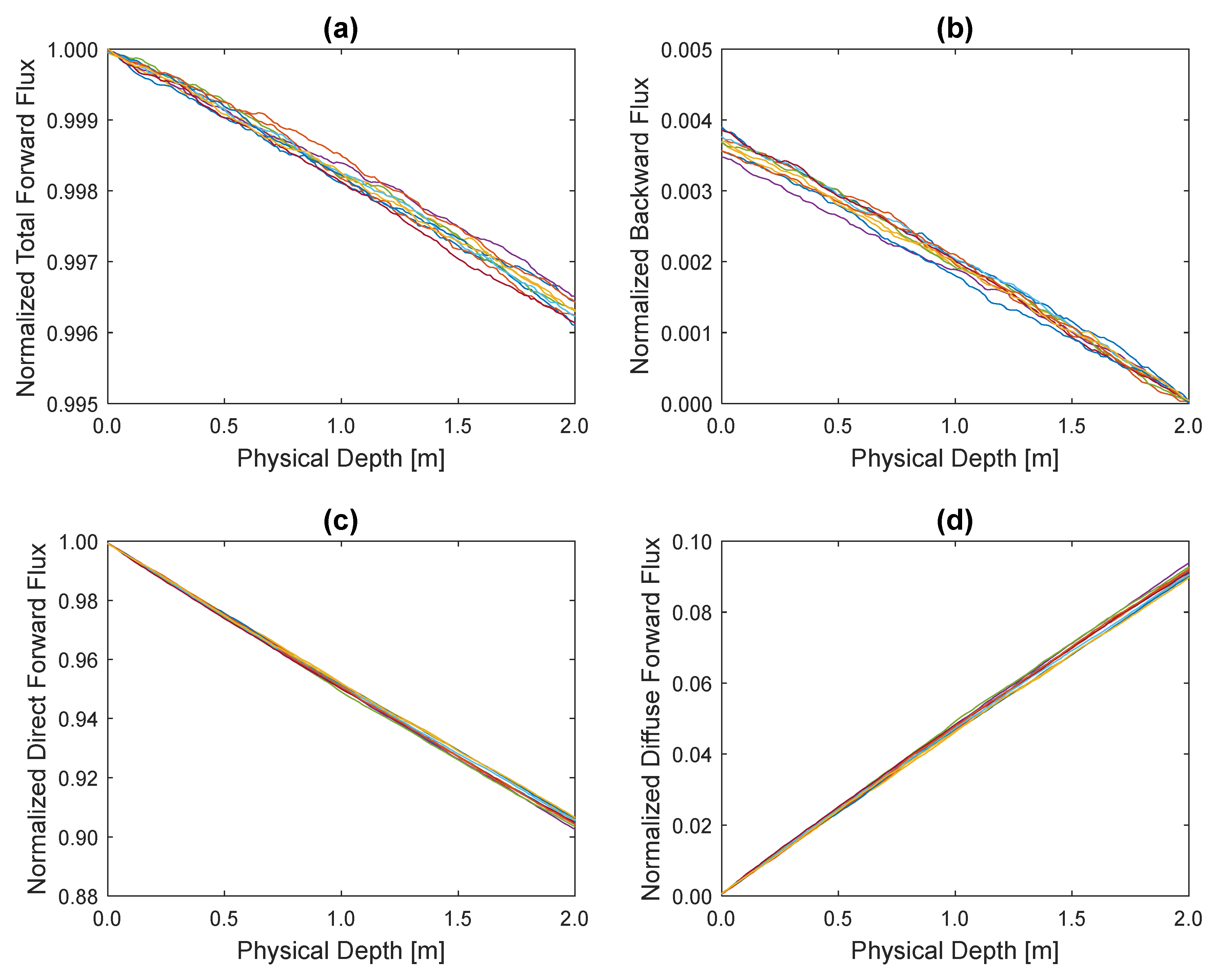
3.1. Scattering MCRT Results for LES Particle Clouds Conditioned on Estimated Optical Thickness

As shown in the expected optical thickness histogram depicted in panel (a) of Figure 2, the mean for all 432 cloud subsamples is close to a value of τ = 0.1 . With numerous cloud subvolumes near this average (expected) optical thickness value, a very tight window ( 0.099 < τ < 0.101 ) can be used to select ten LES output files from all timesteps, which are very similar from the perspective of total optical thickness. These ten LES polydisperse droplet distributions were used to run two sets of MCRT scattering simulations. In the first set, the spatial locations and droplet radii were used directly from the LES export process. Consequently, spatial correlations (on scales greater than the 3.125 cm grid resolution) may exist due to any voids and clusters formed during the turbulent mixing process represented by the LES.
The results of this first LES set, conditioned on τ = 0.1 , are shown in Figure 4. Each of the four panels shows a family of curves for total forward flux, backward flux, diffuse forward, and direct forward flux (clockwise from upper left, respectively). Each curve corresponds to one realization of a subvolume from the LES. An additional dashed curve is shown in panel c to indicate exponential extinction of direct transmission, for comparative purposes. It is notable that the variability along the path length is larger than at the end point (i.e., at 2 m for panels a, c, and d, and at 0 m for the backwards flux in panel b). That is a result of our having conditioned the choice of subvolumes on optical depth. That conditioning allows variation in the fluxes to be attributed to internal spatial variability within a subvolume rather than changes in the mean properties from subvolume to subvolume. How that kind of conditioning can be achieved in an experiment will be discussed later.
In contrast, a second set of scattering simulations (shown in Figure 5) employed the same LES output in terms of the number and size of droplets, but with the droplets redistributed in space. In other words, the spatial locations determined by the LES process were discarded and replaced by uniformly random positions to create corresponding polydisperse distributions without any spatial correlations. A much tighter grouping in the family of curves is evident and is due to the lack of clusters and voids in the spatial distributions. As this set of ten scattering simulations used the same (ten) polydisperse particle size distribution functions as the first set, with only droplet spatial locations being different from the LES-positioned results of Figure 4, the τ values are identical and only spatial correlation can explain the differences between the two figures.
These flux results show stronger deviations within a set (i.e., from the ensemble average) when LES spatial positions are used compared to uniformly random droplet locations. This variability arises from the variation in number density and ‘local’ optical thickness inside a representative LES cloud subvolume compared to its corresponding random counterpart and is illustrated in the top and bottom panels of Figure 6. The effect is further illustrated in Figure 7 by selecting a single LES cloud subvolume and directly comparing the fluxes in the turbulent-correlated clouds (simulated with LES) and the corresponding, idealized homogeneous cloud. It can be seen that in spite of the two subvolumes having the same τ and nearly the same total forward flux, the spatial correlations lead to substantial changes in the partitioning of photons into direct versus diffuse forward flux. There is also a change in backward flux that is proportionally significant. We proceed to analyze the statistics of the four flux components in the next subsection.

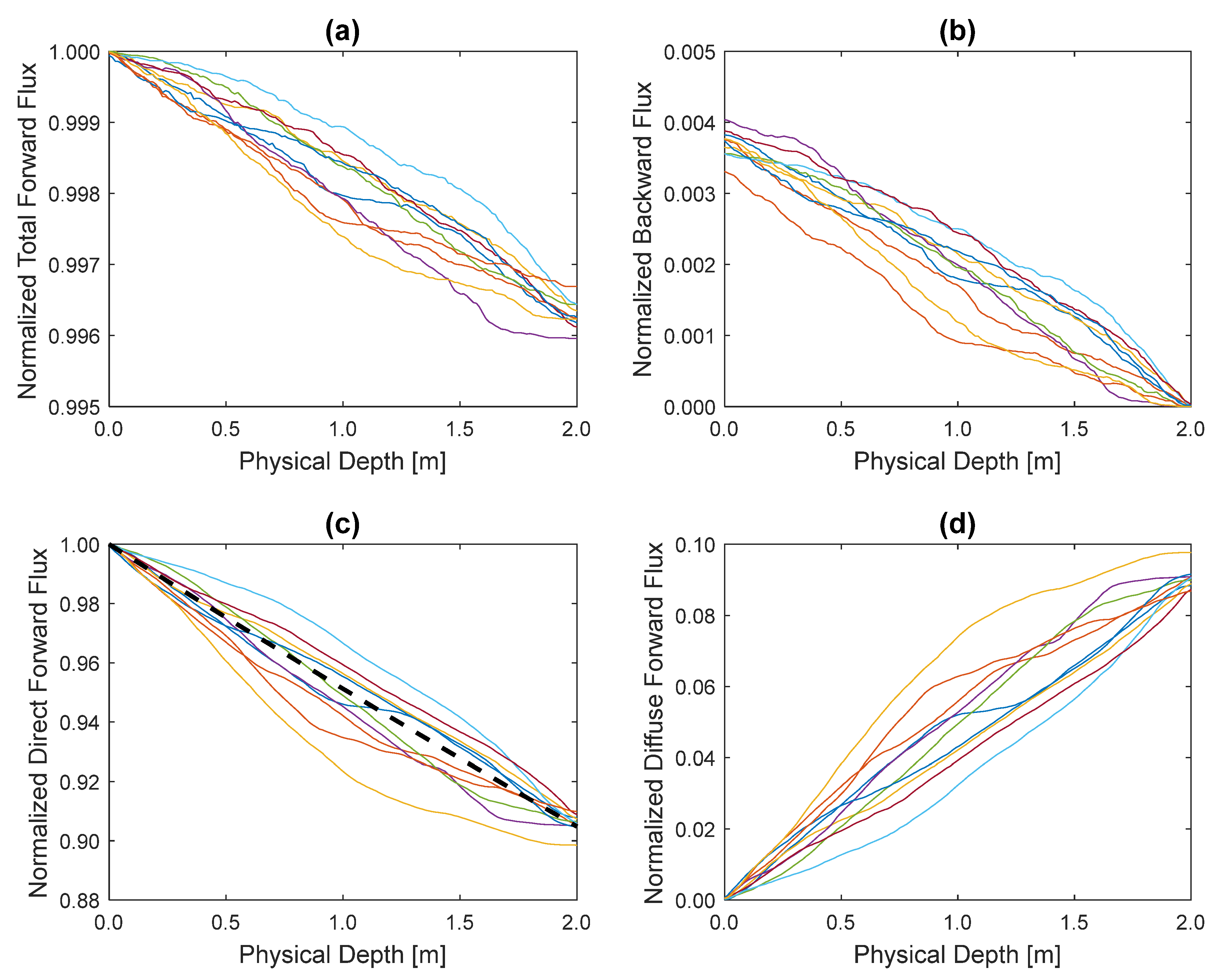
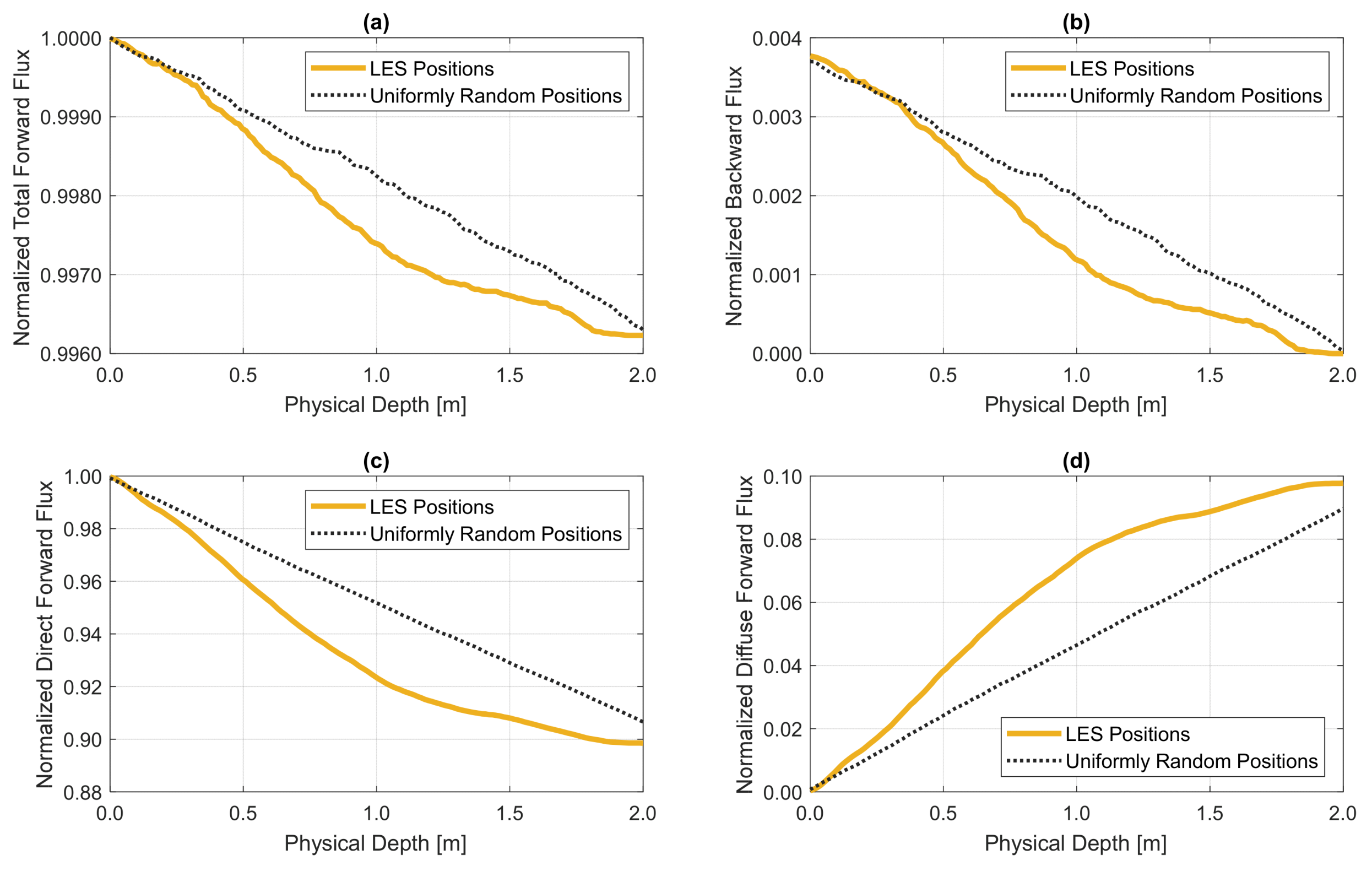
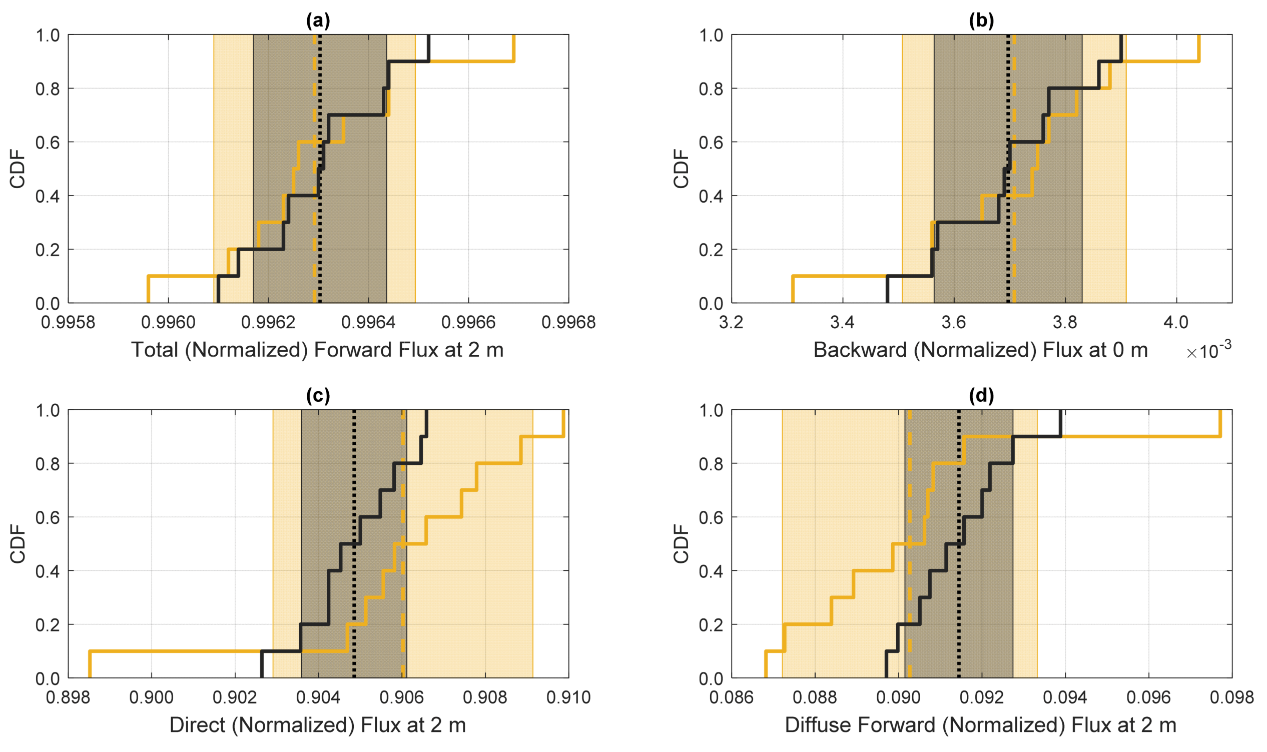
3.2. Statistical Properties of Fluxes with and without Spatial Correlations from Turbulent Mixing

The statistical properties of the ensemble of 10 scattering simulations with nearly equal τ , for both turbulent-clustered and idealized-homogeneous particle distributions, are illustrated in Figure 8. The dashed vertical lines show the mean flux values as they would be measured at the chamber walls: total forward flux (panel a), direct forward flux (panel c), and diffuse forward flux (panel d) measured at 2 m, and backward diffuse flux (panel b) measured at 0 m. The yellow dashed lines display the means of the simulations which employed LES-positioned spatial records, while the black dotted lines indicate the means of those with uniformly random droplet locations. As can be seen in panels (a) and (b) in Figure 8, the total forward and backward flux means are nearly identical; the mean direct and diffuse forward fluxes shown in panel (c) and (d), respectively, display a more substantial change. As predicted in previous works [12,45], spatial correlation typically leads to an increase in direct flux but, at least in the single-scattering regime for forward-scattering particles, a nearly compensating decrease in diffuse forward flux. When backward flux is relatively unchanged, the total forward flux is also largely unchanged due to the offsetting nature of direct and diffuse forward flux.
It is immediately noticeable that the standard deviation of each set is significantly larger for the spatially correlated simulations. This is depicted in Figure 8 by the shaded regions (yellow for the LES-positioned set versus grey for the randomly positioned set) bounded by one standard deviation from the mean (e.g., μ s e t ± σ s e t ). For both total forward flux and backward flux, shown in panels (a) and (b), respectively, the LES-positioned results have an increase by a factor of 2 in standard deviation relative to the uniformly random set: 0.0002 versus 0.0001. Differences in standard deviation for the direct and diffuse forward flux components, shown respectively in panels (c) and (d) of Figure 8, show approximately a factor of 2.4 increase when clustering is present. The standard deviation in direct flux for the uniformly random set is 0.0013, while the corresponding LES-positioned set has a standard deviation of 0.0031.
These scattering simulations, therefore, suggest that while the means from the two sets may be difficult to differentiate in the absence of other information, variations about their respective means (calculated at the extremes of the volume where sensors could most easily be placed) are likely to be larger in the presence of spatial correlation. This has implications for experimental exploration, which are discussed later. It is worth noting that in both panels (c) and (d) of Figure 8, the LES-positioned mean (yellow dashed vertical line) is nearly outside the limits of the grey-filled region. This means that the average direct and diffuse forward flux expected under typical cloud chamber mixing cloud conditions are almost a full standard deviation away from the mean expected in the absence of spatial correlation.

3.3. Variation of Fluxes along the Profiles

The path-dependent properties of variability in flux are also of potential interest from a measurement perspective. It was already shown in Figure 4 that variability along the path is significantly larger for the scattering results accounting for turbulent mixing relative to the homogeneous analogs. Figure 9 shows the 10 individual LES-positioned flux profiles, normalized by their uniformly random spatial counterpart, curve by curve. Using a curve-by-curve, point-by-point division between LES-correlated and spatially uncorrelated results, a ratio can be computed which shows the depth-dependent deviation due only to droplet location (as particle size distributions are identical for both numerator and denominator). A value of unity indicates a perfect match at a given physical depth along the propagation path, suggesting negligible impact from spatial correlation, while values above and below one suggest increases and decreases (respectively) from the homogeneous case due to spatial correlations. Effects of spatial correlation are somewhat exaggerated for backward and diffuse forward flux, since division by small flux numbers for the same absolute flux difference results in a larger deviation ratio.
Examining these ratio results at the most convenient sensor locations (a depth of 2 m for all forward flux components, and a depth of 0 m for backward flux) allows us to estimate both the steady and variable impacts of spatial correlation. Positive shifts of the mean (ratios above 1) correspond to increases in average flux sensed at that location, while negative shifts (ratios below 1) indicate a reduction in average flux. The mean flux ratios had only small variations from unity, with direct forward and backward fluxes slightly over 1 and diffuse forward flux slightly less than 1. Larger standard deviations, indicating higher fluctuations about the mean flux ratios, represent a more variable impact of spatial clustering. The backward and diffuse forward flux components are the most sensitive to the presence of spatial correlations, with a dispersion (standard deviation normalized by the mean) of several percent (ratios of 0.0657 and 0.0417, respectively). The impact on total forward and direct flux is not significant, with a statistical dispersion of less than one percent (0.0002 and 0.0042, respectively).
Another aspect of Figure 9 that is intriguing from a measurement perspective is the enhanced variance along the path, as compared to that at the chamber surfaces (i.e., between the limits of 0 and 2 m). Diffuse forward and backward fluxes (panels d and b, respectively) exhibit fluctuations of over plus–minus 50%. Peak fluctuations appear at approximately 0.5 m for diffuse forward flux and at approximately 1.5 m for diffuse backward flux. Given that the correlation length for clusters in the LES are approximately 0.2 m, we infer that the peaks occur approximately two correlation lengths from the incident surface for diffuse forward flux and approximately two correlation lengths from the far surface for diffuse backward flux. These could be considered optimal locations for measuring fluctuations, assuming that the measurement is conditioned on τ as is done in this analysis of the Monte Carlo simulation of scattering.

4. Implications for Measurement of Light Propagation in a Convection Cloud Chamber

We started this paper by stating that our purpose is to take a step toward experimental verification by exploring computationally whether deviations from standard radiative transfer for a homogeneous medium can plausibly be detected in a laboratory-generated cloud containing spatial correlations in droplet position due to turbulent mixing. In this section, we turn from presentation of simulation results to the implications of those results for experiments, with a focus on what quantities can be measured that would give indications of departures from exponential extinction due to droplet spatial correlations. The cloud chamber turbulence simulations and the Monte Carlo ray tracing calculations have all been carried out using the parameters of the Pi convection cloud chamber, so the discussion here maintains that context. In the Pi Chamber, mixing clouds with steady state microphysical properties can be sustained for hours and the droplet number size distributions can be measured throughout the life of the cloud. An experimental setup similar in geometry to the simulations described here is now discussed. A normally incident, collimated visible light beam can be used to illuminate the chamber-confined cloud, as was done in prior experiments on image blurring due to light scattering by cloud droplets [17]. The total forward flux could be monitored with a photodiode array or digital camera on the opposite side of the chamber, as well as a reference diode to obtain the incident flux. A photodiode array or camera on the light-input side would allow for measurement of backward flux. Details of the angular extent of these detectors and how to optically separate forward direct and forward diffuse flux are not considered at this stage because making an angle-dependent analysis is much more computationally expensive for the Monte Carlo method. The light propagation time is small compared to all turbulence time scales, so a detector with sufficiently short integration time (less than the Kolmogorov time scale, which is of order 100 ms) will ensure the frozen field assumption is valid. As the properties of the turbulent mixing cloud fluctuate in time, the effective optical thickness (measured using the fractional amount of light exiting the chamber after propagating through the particle distribution) will vary as well. Measurements separated by more than one correlation time can be considered independent, allowing for ensemble averaging. Relevant correlation times are the turbulence large eddy time, typically several to 10 s, and the chamber circulation time, typically about 1 min; the Pi Chamber allows steady state mixing clouds to be generated for many hours, allowing for plentiful independent samples. Using the LES as a guide, we can anticipate that taking several hundred samples should be adequate to enable analysis of conditional statistics.
The analysis of simulation results was carried out by first conditioning the selection of samples on the optical thickness τ . That is a simple matter for simulation, but in a laboratory experiment requires careful consideration. One approach is to simultaneously measure the droplet number size distribution and use the measurement of number concentration and mean-squared diameter to calculate the expected τ . This is not entirely adequate with current methods, however, because the measured values are local, not distributed along the entire path. One approach would be to use a combination of infrared absorption and visible light extinction measurements along the path to obtain τ at the appropriate wavelength. A more practical approach, suggested by the analysis made in the previous section, is to use total forward flux as a surrogate for effective optical thickness. By measuring the direct and diffuse forward flux independently, conditioning based on the total forward flux becomes possible. This would allow analysis of the statistics (e.g., mean and standard deviation) of the forward direct and forward diffuse flux components for cloud paths with the same optical thickness (as determined using total forward flux). These means and standard deviations could then be compared to values predicted using the measured, time-average particle size distribution function and a uniformly random position assumption to detect and assess the effect of particle clustering. It was also noted in the previous section that the backward diffuse flux is sensitive to clustering, both in terms of its mean and fluctuations. It, therefore, would be advantageous to have an additional detector on the light-input side of the chamber for that purpose. Again, the measurement of total forward flux would be used in conditional selection of samples for the analysis of backward diffuse flux statistics.
In Figure 8, we saw that measured means of forward direct and diffuse radiation may be shifted by nearly one standard deviation of the “homogeneous” expectation. A focus on these mean values would, therefore, be of interest. The fluctuations themselves, illustrated in the same figure, seem most compelling for detecting and characterizing deviations from expected propagation for a homogeneous medium. Once detector sizes and experiment geometry are determined, the Monte Carlo ray tracing code used in this study can be run to obtain estimates for specific experimental conditions, thereby allowing the expected changes in mean and standard deviation to be determined. In fact, we anticipate that a more detailed exploration of the angular dependence of the diffuse light will be of interest in future investigations. Depending on the droplet size distribution, and the associated strength of forward scattering, looking at several near-forward angle ranges could be particularly insightful.
The simulation results also give an indication of the detector sensitivity or dynamic range that would be required for experiments to investigate the influence of mixing and the resulting droplet clustering on radiative fluxes. With a nominal optical depth of 0.1 (easily achievable in a sustainable mixing cloud), direct flux was observed to increase from less than 90.5% of incident illumination to 90.6% when realistic clustering was present. Furthermore, the standard deviation of the same measurement increased from 0.0013 to 0.0031 (a factor of 2.4). In a similar fashion, the mean diffuse forward flux decreased from 9.15% of incident illumination to 9.03%, but the standard deviation increased from 0.0013 to 0.0031 (same factor of 2.4). Detectors sensitive enough to measure the levels of illumination of interest, with sufficient resolution to reliably measure variations at the 0.1% level, should be capable of discriminating between subtly different means. The strongly dissimilar standard deviations will be much easier to detect.
Considering the simulation findings illustrated in Figure 9, it also may be advantageous to place detectors within the chamber. It was noted in the discussion of that figure that about two turbulence correlation lengths from the chamber surfaces may be the optimal location for measurement of fluctuations in forward diffuse and backward diffuse radiation. Again, the droplet number size distribution would need to be measured so that the homogeneous cloud τ could be calculated, as well as the associated path dependence of flux. With a suitable traverse system, one could plausibly measure the mean and standard deviation along a full profile of forward and backward diffuse flux. Here, we again note the advantage of the mixing cloud mechanism used in the Pi Chamber, allowing for statistically stationary cloud conditions that allow for ensemble averaging in time.
Another possible laboratory setup for a cloud chamber experiment to explore particle clustering would be to employ a series of mirrors and beam splitters to split incident light into multiple paths. One such test might be to create two simultaneous but different double pass (four meter) propagation paths, one that is rerouted back through the same optical path and another that is redirected such that the second pass traverses a different region of the mixing cloud. Flux values would be recorded after photons traverse the chamber and then, back again for a total propagation distance of four meters. A comparison of measured flux components from two different double pass beams would be performed; if the cloud volume is indeed homogeneous, both double pass beams should register similar statistics. However, statistically significant differences between the two would allow the homogeneity of the entire cloud volume to be assessed.

5. Discussion and Conciusions

Radiative transfer through a dilute medium, and the resulting optical transmissivity, is dependent on the number and size of particles in the distribution. If spatial correlations exist in particle locations, clusters and voids may exist on scales of the same order as or smaller than the optical mean free path (as defined for a uniform medium). In the scattering-dominated regime, where absorption is essentially nonexistent, radiation is either transmitted directly (without any particle interaction) or diffusely (photons change propagation direction but continue traversing the medium).
In this work, we have investigated direct and diffuse radiative transfer in a medium with spatially correlated scattering particles using a ballistic photon MCRT model. Our simulations explored the forward-dominant scattering regime that is typical of atmospheric clouds. The results are framed in the context of direct and diffuse forward and backward fluxes. Polydisperse LES particle distributions were generated with boundary conditions realizable in the Pi Cloud Chamber to aid the design of an experimental setup meant to measure the presence and impact of spatial correlation.
We found much more cloud-to-cloud variation when the LES-positioned droplet locations were employed (as opposed to uniformly random positions). This was especially evident in the center of the clouds at a physical depth of one meter (see Figure 4 and Figure 5), but the impact of spatial correlation was still apparent at the propagation endpoints (edges of the confined geometry). The change in mean total forward flux and backward flux for the ten cloud sections analyzed (chosen for their estimated optical thickness of 0.1) was negligible. Panels (a) and (b) of Figure 8 indicate that while the standard deviation of these flux components is 1.5–2 times larger in simulations with correlated particle positions, the means are essentially the same.
However, the direct and diffuse forward flux results shown respectively in panels (c) and (d) of Figure 8 vary in both mean and standard deviation. The standard deviation of the results set with LES-positioned droplets is approximately 2.4 times larger than when spatial correlation is removed by using uniformly random particle locations. Additionally, the mean of these flux components is separated sufficiently such that the mean values of the LES-positioned results are almost a standard deviation away from the mean values from the uncorrelated distributions. If we denote the spatially correlated and uncorrelated direct flux mean values (respectively) as μ L E S and μ h o m o g , and the standard deviation values as σ L E S and σ h o m o g , we observe in Figure 8 that the direct and diffuse forward flux means are empirically related by the expressions
μ L E S d i r e c t μ h o m o g d i r e c t + σ h o m o g d i r e c t
and
μ L E S d i f f F o r w μ h o m o g d i f f F o r w σ h o m o g d i f f F o r w .
With flux means separated by 1–2% and significantly different standard deviations, it seems that the direct and diffuse forward flux components are the most distinguishable. This conclusion is consistent with the findings of a recent study [12], even though that work focused on monodisperse distributions (with τ ~ 1 and strong particle clustering) and the current study (with τ ~ 0.1 and weaker particle clustering) employs realistic polydisperse distributions from large eddy simulations (LES).
When the entire set of LES-positioned results are normalized by the uncorrelated results, curve-by-curve at each physical depth along the propagation path, the means of the resulting flux component ratios indicate the average fractional increase or decrease in radiative transfer due to spatial correlation. The mean flux ratios observed at the chamber endpoints of Figure 9 show that while the total forward flux is essentially unchanged, the flux ratios of the direct, diffuse forward, and backward components are 1.001, 0.988, and 1.004 (respectively). While the backward flux has a larger percentage change than the direct flux, the absolute difference is very small and might require a high signal-to-noise ratio (SNR) to measure with confidence. The largest percentage change is the reduction in diffuse forward flux, due to the fact that while the absolute differences in the direct and diffuse forward flux are similar, the denominator is smaller for the diffuse forward (9% of incident intensity vs. 90% of incident intensity for direct). The observed flux ratio standard deviation values suggest the variation in impact on flux ratio due to spatial correlation.
The flux results presented in this work suggest several possible experimental setups that could be successful at detecting the presence (and potentially, the magnitude) of particle clustering. In the Pi Chamber, mixing clouds can be sustained for hours and the particle size distribution function can be measured throughout the life of the cloud. A normally incident, collimated visible light beam could be used to illuminate the chamber-confined cloud, and the total forward flux could be monitored on the opposite side of the chamber. The frozen field assumption is valid due to speed of light measurements, and the statistical stationarity of cloud properties allows a large number of values to be recorded for statistical convergence of the measurements. As the properties of the mixing cloud fluctuate in time, the effective optical thickness will vary as well. Effective optical thickness is found to be related to the total forward (direct plus diffuse) flux. By measuring the direct and diffuse forward flux separately, while also monitoring total forward flux, conditioning based on total forward flux (and, as a result, total effective optical thickness) becomes possible. This would allow analysis of the statistics, e.g., mean and standard deviation, of the forward direct and diffuse fluxes as well as backward flux, for cloud paths with the same optical thickness. These measured flux statistics can be compared to values predicted using a simultaneously-measured, time-averaged cloud droplet size distribution function and a uniformly random position assumption to test the likelihood (and possibly estimate the magnitude) of particle clustering.
Finally, we consider the value of experiments in general, relative to simulations. One aspect, of course, is to evaluate the suitability of the assumptions underlying the simulation approach. The experiments contain all of the physics, so possible deviations resulting from inadequacy of geometric ray tracing or turbulence representation can be identified. In addition, and just as importantly, experiments can be easily run under a wide range of microphysical conditions and experiment geometries to explore the broad parameter space that exists for this problem. For example, the angle at which detectors are set, and the angular width of detectors can be altered, whereas Monte Carlo ray tracing simulations with high angular resolution are exceedingly expensive to run. The Pi Chamber allows a wide range of cloud microphysical properties to be generated, by varying the size and number concentration (and even composition) of aerosol particles [46]. Thus, the cloud optical thickness can be varied, and the same optical thickness achieved by different microphysical properties, such as small numbers of large droplets or large numbers of small droplets, can be explored. The Pi Chamber also allows for a range of turbulence intensities to be explored, by changing the imposed temperature difference [14]. More succinctly, the experiments will allow the following advantages: they allow a wide range of turbulence and microphysical properties to be explored, with flexible measurement geometry, and allow for long time sampling to obtain suitable statistical convergence.

Author Contributions

Conceptualization, W.H.C., M.L.L., C.D.P. and R.A.S.; methodology, M.L.L., C.D.P. and R.A.S.; software, C.D.P. and S.T.; validation, M.L.L., C.D.P., R.A.S. and S.T.; formal analysis, M.L.L., C.D.P. and R.A.S.; writing, W.H.C., M.L.L., C.D.P. and R.A.S. All authors have read and agree to the published version of the manuscript.

Funding

This research was funded by Air Force Research Laboratory (AFRL) agreement number FA9453-16-1-0083, the South Carolina Space Grant Research and Education Awards Program, as well as by National Science Foundation (NSF) grants AGS-1532977, AGS-1754244, and AGS-1823334. The U.S. Government is authorized to reproduce and distribute reprints for Governmental purposes notwithstanding any copyright notation thereon. The views and conclusions contained herein are those of the authors and should not be interpreted as necessarily representing the official policies or endorsements, either expressed or implied, of Air Force Research Laboratory (AFRL) or the U.S. Government.

Acknowledgments

We thank A. B. Kostinski for many helpful discussions that inspired this work. Portage, a high-performance computing infrastructure at Michigan Technological University, was used in obtaining results presented in this publication.

Conflicts of Interest

The authors declare no conflict of interest. The funders had no role in the design of the study; in the collection, analyses, or interpretation of data; in the writing of the manuscript, or in the decision to publish the results.

References

  1. Borovoi, A.G. Radiative transfer in inhomogeneous media. Dokl. Akad. Nauk SSSR 1984, 276, 1374–1378. [Google Scholar]
  2. Kostinski, A.B.; Jameson, A.R. On the Spatial Distribution of Cloud Particles. J. Atmos. Sci. 2000, 57, 901–915. [Google Scholar] [CrossRef] [Green Version]
  3. Kostinski, A.B.; Shaw, R.A. Scale-dependent droplet clustering in turbulent clouds. J. Fluid Mech. 2001, 434, 389–398. [Google Scholar] [CrossRef]
  4. Marshak, A.; Davis, A.B. 3D Radiative Transfer in Cloudy Atmospheres; Springer: Berlin, Germany, 2005; ISBN 978-3-540-23958-1. [Google Scholar]
  5. Davis, A.B.; Marshak, A. Photon propagation in heterogeneous optical media with spatial correlations: Enhanced mean-free-paths and wider-than-exponential free-path distributions. J. Quant. Spectrosc. Radiat. Transf. 2004, 84, 3–34. [Google Scholar] [CrossRef]
  6. Larsen, E.W.; Vasques, R. A generalized linear Boltzmann equation for non-classical particle transport. J. Quant. Spectrosc. Radiat. Transf. 2011, 112, 619–631. [Google Scholar] [CrossRef]
  7. Davis, A.B.; Marshak, A.; Gerber, H.; Wiscombe, W.J. Horizontal structure of marine boundary layer clouds from centimeter to kilometer scales. J. Geophys. Res. Atmos. 1999, 104, 6123–6144. [Google Scholar] [CrossRef]
  8. Shaw, R.A. Particle-turbulence interactions in atmospheric clouds. Annu. Rev. Fluid Mech. 2003, 35, 183–227. [Google Scholar] [CrossRef] [Green Version]
  9. Kostinski, A.B. On the extinction of radiation by a homogeneous but spatially correlated random medium. J. Opt. Soc. Am. A JOSAA 2001, 18, 1929–1933. [Google Scholar] [CrossRef]
  10. Larsen, M.; Clark, A. On the link between particle size and deviations from the Beer–Lambert–Bouguer law for direct transmission. J. Quant. Spectrosc. Radiat. Transf. 2014, 133, 646–651. [Google Scholar] [CrossRef]
  11. Frankel, A.; Iaccarino, G.; Mani, A. Optical depth in particle-laden turbulent flows. J. Quant. Spectrosc. Radiat. Transf. 2017, 201, 10–16. [Google Scholar] [CrossRef]
  12. Packard, C.D.; Larsen, M.L.; Cantrell, W.H.; Shaw, R.A. Light scattering in a spatially-correlated particle field: Role of the radial distribution function. J. Quant. Spectrosc. Radiat. Transf. 2019, 236, 106601. [Google Scholar] [CrossRef]
  13. Bohren, C.F.; Clothiaux, E.E. Fundamentals of Atmospheric Radiation: An Introduction with 400 Problems; Wiley-VCH: Weinheim, Germany, 2011; ISBN 978-3-527-40503-9. [Google Scholar]
  14. Chang, K.; Bench, J.; Brege, M.; Cantrell, W.; Chandrakar, K.; Ciochetto, D.; Mazzoleni, C.; Mazzoleni, L.R.; Niedermeier, D.; Shaw, R.A. A laboratory facility to study gas-aerosol-cloud interactions in a turbulent environment: The Π Chamber. Bull. Am. Meteorol. Soc. 2016. [Google Scholar] [CrossRef]
  15. Thomas, S.; Ovchinnikov, M.; Yang, F.; van der Voort, D.; Cantrell, W.; Krueger, S.K.; Shaw, R.A. Scaling of an Atmospheric Model to Simulate Turbulence and Cloud Microphysics in the Pi Chamber. J. Adv. Model. Earth Syst. 2019, 11, 1981–1994. [Google Scholar] [CrossRef] [Green Version]
  16. Shaw, R.A.; Kostinski, A.B.; Lanterman, D.D. Super-exponential extinction of radiation in a negatively correlated random medium. J. Quant. Spectrosc. Radiat. Transf. 2002, 75, 13–20. [Google Scholar] [CrossRef] [Green Version]
  17. Packard, C.D.; Shaw, R.A.; Cantrell, W.H.; Kinney, G.M.; Roggemann, M.C.; Valenzuela, J.R. Measuring the detector-observed impact of optical blurring due to aerosols in a laboratory cloud chamber. JARS 2018, 12, 042404. [Google Scholar] [CrossRef]
  18. Danielson, R.E.; Moore, D.R.; van de Hulst, H.C. The Transfer of Visible Radiation through Clouds. J. Atmos. Sci. 1969, 26, 1078–1087. [Google Scholar] [CrossRef] [Green Version]
  19. Plass, G.N.; Kattawar, G.W. Monte Carlo Calculations of Light Scattering from Clouds. Appl. Opt. 1968, 7, 415–419. [Google Scholar] [CrossRef]
  20. Collins, D.G.; Blättner, W.G.; Wells, M.B.; Horak, H.G. Backward Monte Carlo Calculations of the Polarization Characteristics of the Radiation Emerging from Spherical-Shell Atmospheres. Appl. Opt. 1972, 11, 2684–2696. [Google Scholar] [CrossRef]
  21. Sobol’, I.M. The Monte Carlo Method. Popular Lectures in Mathematics; The University of Chicago Press: Chicago, IL, USA, 1974. [Google Scholar]
  22. Marchuk, G.I.; Mikhailov, G.A.; Nazaraliev, M.A.; Darbinjan, R.A.; Kargin, B.A.; Elepov, B.S. The Monte Carlo Methods in Atmospheric Optics; Springer: Berlin/Heidelberg, Germany, 1980; Volume 12. [Google Scholar]
  23. Cole, J.N.S. Assessing the importance of unresolved cloud-radiation interactions in atmospheric global climate models using the multiscale modelling framework. Ph.D. Thesis, Department of Meteorology, The Pennsylvania State University, State College, PA, USA, 2005. [Google Scholar]
  24. Henyey, L.G.; Greenstein, J.L. Diffuse radiation in the galaxy. Astrophys. J. 1941, 93, 70–83. [Google Scholar] [CrossRef]
  25. Thomas, G.E.; Stamnes, K. Radiative Transfer in the Atmosphere and Ocean; Cambridge University Press: Cambridge, UK, 1996; ISBN 978-0-521-40124-1. [Google Scholar]
  26. Ishimaru, A. Wave Propagation and Scattering in Random Media; IEEE Press: New York, NY, USA, 1997; ISBN 978-0-7803-4717-5. [Google Scholar]
  27. Frankel, A.; Iaccarino, G.; Mani, A. Convergence of the Bouguer–Beer law for radiation extinction in particulate media. J. Quant. Spectrosc. Radiat. Transf. 2016, 182, 45–54. [Google Scholar] [CrossRef]
  28. Banko, A.J.; Villafañe, L.; Kim, J.H.; Esmaily, M.; Eaton, J.K. Stochastic modeling of direct radiation transmission in particle-laden turbulent flow. J. Quant. Spectrosc. Radiat. Transf. 2019, 226, 1–18. [Google Scholar] [CrossRef]
  29. Mishchenko, M.I. Multiple scattering, radiative transfer, and weak localization in discrete random media: Unified microphysical approach. Rev. Geophys. 2008, 46. [Google Scholar] [CrossRef] [Green Version]
  30. Mishchenko, M.I.; Dlugach, J.M.; Yurkin, M.A.; Bi, L.; Cairns, B.; Liu, L.; Panetta, R.L.; Travis, L.D.; Yang, P.; Zakharova, N.T. First-principles modeling of electromagnetic scattering by discrete and discretely heterogeneous random media. Phys. Rep. 2016, 632, 1–75. [Google Scholar] [CrossRef] [PubMed] [Green Version]
  31. Matérn, B. Poisson Processes in the Plane and Related Models for Clumping and Heterogeneity. Ph.D. Thesis, NATO Advanced Study Institute on Statistical Ecology. Pennsylvania State University, State College, PA, USA, 1972. [Google Scholar]
  32. Martínez, V.J.; Saar, E. Statistics of the Galaxy Distribution; CRC Press: Boca Raton, FL, USA, 2002. [Google Scholar]
  33. Larsen, M.L.; Briner, C.A.; Boehner, P. On the Recovery of 3D Spatial Statistics of Particles from 1D Measurements: Implications for Airborne Instruments. J. Atmos. Ocean. Technol. 2014, 31, 2078–2087. [Google Scholar] [CrossRef]
  34. Khairoutdinov, M.F.; Randall, D.A. Cloud Resolving Modeling of the ARM Summer 1997 IOP: Model Formulation, Results, Uncertainties, and Sensitivities. J. Atmos. Sci. 2003, 60, 607–625. [Google Scholar] [CrossRef]
  35. Khain, A.; Pokrovsky, A.; Pinsky, M.; Seifert, A.; Phillips, V. Simulation of Effects of Atmospheric Aerosols on Deep Turbulent Convective Clouds Using a Spectral Microphysics Mixed-Phase Cumulus Cloud Model. Part I: Model Description and Possible Applications. J. Atmos. Sci. 2004, 61, 2963–2982. [Google Scholar] [CrossRef] [Green Version]
  36. Niedermeier, D.; Chang, K.; Cantrell, W.; Chandrakar, K.K.; Ciochetto, D.; Shaw, R.A. Observation of a link between energy dissipation rate and oscillation frequency of the large-scale circulation in dry and moist Rayleigh-B\’enard turbulence. Phys. Rev. Fluids 2018, 3, 083501. [Google Scholar] [CrossRef]
  37. Chandrakar, K.K.; Cantrell, W.; Chang, K.; Ciochetto, D.; Niedermeier, D.; Ovchinnikov, M.; Shaw, R.A.; Yang, F. Aerosol indirect effect from turbulence-induced broadening of cloud-droplet size distributions. PNAS 2016, 113, 14243–14248. [Google Scholar] [CrossRef] [Green Version]
  38. Chandrakar, K.K.; Cantrell, W.; Ciochetto, D.; Karki, S.; Kinney, G.; Shaw, R.A. Aerosol removal and cloud collapse accelerated by supersaturation fluctuations in turbulence. Geophys. Res. Lett. 2017, 44, 4359–4367. [Google Scholar] [CrossRef] [Green Version]
  39. Desai, N.; Chandrakar, K.K.; Chang, K.; Cantrell, W.; Shaw, R.A. Influence of microphysical variability on stochastic condensation in a turbulent laboratory cloud. J. Atmos. Sci. 2018, 75, 189–201. [Google Scholar] [CrossRef]
  40. Jameson, A.R.; Larsen, M.L. The variability of the rainfall rate as a function of area. J. Geophys. Res. Atmos. 2016, 121, 746–758. [Google Scholar] [CrossRef] [Green Version]
  41. Saw, E.-W.; Shaw, R.A.; Salazar, J.P.L.C.; Collins, L.R. Spatial clustering of polydisperse inertial particles in turbulence: II. Comparing simulation with experiment. New J. Phys. 2012, 14, 105031. [Google Scholar] [CrossRef] [Green Version]
  42. Lu, J.; Nordsiek, H.; Shaw, R.A. Clustering of settling charged particles in turbulence: Theory and experiments. New J. Phys. 2010, 12, 123030. [Google Scholar] [CrossRef] [Green Version]
  43. Saw, E.-W.; Salazar, J.P.L.C.; Collins, L.R.; Shaw, R.A. Spatial clustering of polydisperse inertial particles in turbulence: I. Comparing simulation with theory. New J. Phys. 2012, 14, 105030. [Google Scholar] [CrossRef]
  44. Matsuda, K.; Onishi, R.; Kurose, R.; Komori, S. Turbulence effect on cloud radiation. Phys. Rev. Lett. 2012, 108, 224502. [Google Scholar] [CrossRef] [Green Version]
  45. Petty, G.W. Area-Average Solar Radiative Transfer in Three-Dimensionally Inhomogeneous Clouds: The Independently Scattering Cloudlet Model. J. Atmos. Sci. 2002, 59, 2910–2929. [Google Scholar] [CrossRef] [Green Version]
  46. Chandrakar, K.K.; Cantrell, W.; Shaw, R.A. Influence of Turbulent Fluctuations on Cloud Droplet Size Dispersion and Aerosol Indirect Effects. J. Atmos. Sci. 2018, 75, 3191–3209. [Google Scholar] [CrossRef]
Figure 1. The entire volume of the simulated cloud chamber (2 × 2 × 1 m) is depicted with a dashed rectangular prism outline. Inside this volume, 48 high aspect ratio cuboids are extracted for optical analysis. Each cuboid, or cloud subsample, has dimensions of 0.2 × 0.2 × 2.0 m; 24 subsamples are taken from each horizontal direction in the chamber. Here, the dotted grids show the ends of the 48 cloud subsamples, with only a single 3D subsample (rectilinear parallelepiped) portrayed in each direction; the other 46 are hidden for the sake of clarity.
Atmosphere 11 00837 g001
Figure 2. (a) Histogram of optical thickness from 432 LES output files. Values in the distribution range from 0.02 to 0.14, with an average optical thickness of 0.09, a standard deviation of 0.02, and a relative dispersion of 0.222. (b) Histogram of subvolume mean number density from 432 LES output files. Values in the distribution range from 243 to 1227 droplets per cubic centimeter, with an average of 846 cm−3, a standard deviation of 174 cm−3, and a relative dispersion of 0.206. (c) Histogram of subvolume mean geometric cross section from 432 LES output files. Values range from 22 to 30 μm2, with a mean of 26.4 μm2, a standard deviation of 1.27 μm2, and a relative dispersion of 0.048.
Atmosphere 11 00837 g002
Figure 3. (a) Scatter plot showing high correlation (R2 = 0.97) between mean volumetric number density and total optical thickness. This suggests that LES output files chosen based on similar number densities are highly likely to have very similar total optical thicknesses. (b) Scatter plot showing correlation (R2 = 0.49) between mean geometric cross section and total optical thickness. This suggests that LES output files chosen based on similar mean geometric cross section are likely to be more weakly coupled to total optical thickness.
Atmosphere 11 00837 g003
Figure 4. Depth-dependent flux curves for ten LES polydisperse spatial distributions, chosen to be very near an expected total optical thickness of 0.1. Spatial positions come directly from LES output records. Panels (a)–(d) show the four flux components including total forward, backward, direct forward and diffuse forward (respectively). An additional dashed curve was added to panel c to indicate Beer–Lambert law direct transmission, for comparative purposes. Theoretical predictions for the other panels are difficult due to the complex nature of our simulations (e.g., periodic boundary conditions, lack of a true plane parallel scenario, etc.). See [12] for a comparison of the Monte Carlo approach to two-stream theory and the accompanying discussion. It should be noted that convergence at the end of the optical path is expected, and is largely predetermined, because of preconditioning the LES distribution selection based on expected optical thickness τ = 0.1 ± 0.001 .
Atmosphere 11 00837 g004
Figure 5. Depth-dependent flux curves for ten LES polydisperse spatial distributions, chosen to be very near a total optical thickness of 0.1. Spatial positions are uniformly random. Again, panels (a)–(d) show four flux components: total forward, backward, direct forward and diffuse forward (respectively).
Atmosphere 11 00837 g005
Figure 6. A random selection of 10,000 particles from each of the spatial distributions whose flux results are shown in Figure 7. The representative illustration in the top panel shows LES-positioned droplet locations, with high number density in the first meter and a large void between 1.0 and 1.2 m. The bottom panel shows the same number of particles which have been placed in a uniformly random fashion.
Atmosphere 11 00837 g006
Figure 7. Normalized flux components from two scattering simulations which both employ the same particle size distribution function. As before, panels (a)–(d) show total forward, backward, direct forward and diffuse forward fluxes (respectively). The thick yellow line results from the use of LES-positioned droplet locations, while the dotted black line results from the use of uniformly random particle positions.
Atmosphere 11 00837 g007
Figure 8. Solid, stepped lines are Cumulative Density Functions (CDFs) calculated from the flux results at the simulated boundaries of the two 10-element sets of scattering simulations with expected optical depths near 0.1, one with LES-positioned particles with spatial correlations arising from turbulent mixing (yellow) and the other with uniformly random droplet locations (black). Both sets of results employed the same LES-exported particle size distribution functions, meaning the only difference between the two sets is the use of LES spatial positions vs. uniformly random positions (same droplet size distribution). Panel (a) is total forward flux, panel (b) is backward flux, panel (c) is direct forward flux, and panel (d) is diffuse forward flux. All fluxes are normalized by the incident illumination flux. Mean flux values are shown with dashed and dotted vertical lines, and shaded areas denote plus–minus one standard deviation to show the variation in flux values. All statistics correspond to virtual measurements at 2 m (end surface of the chamber) for all forward fluxes and at 0 m (incoming surface of the chamber) for the backward flux.
Atmosphere 11 00837 g008
Figure 9. Point-by-point ratios calculated between flux results from LES-positioned droplet locations and those where uniformly random particle locations are used, shown as a function of physical depth. Values of 1 indicate a perfect match at a given physical depth, suggesting negligible impact from spatial correlation. Values above and below 1 suggest increases and decreases (respectively) from the homogeneous case due to spatial correlation. Note that the impact of spatial correlation is much larger in the center of the chamber, while the ratio curves tend to converge at the propagation endpoints (since the effective optical thickness values are very similar). As in several previous figures, panels (a)–(d) show total forward, backward, direct forward and diffuse forward fluxes (respectively).
Atmosphere 11 00837 g009

