A Numerical Study of Aeolian Sand Particle Flow Incorporating Granular Pseudofluid Optimization and Large Eddy Simulation


Abstract
1. Introduction
2. Continuum Models for Two Phases
3. Conditions for Simulation
4. Results and Discussion
4.1. Distribution of Sand Concentration
4.2. Sand Velocity
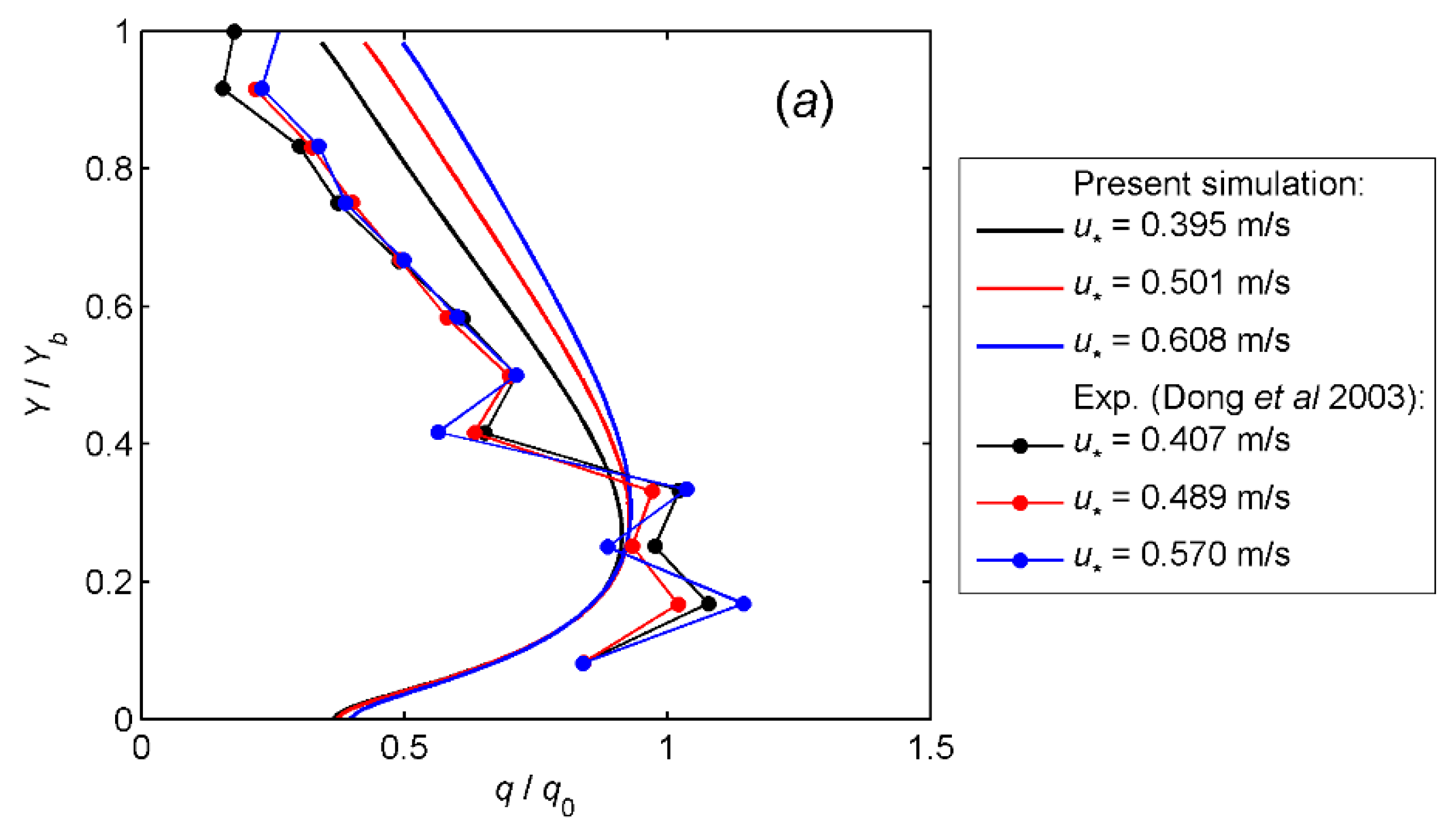
4.3. Sand Flux
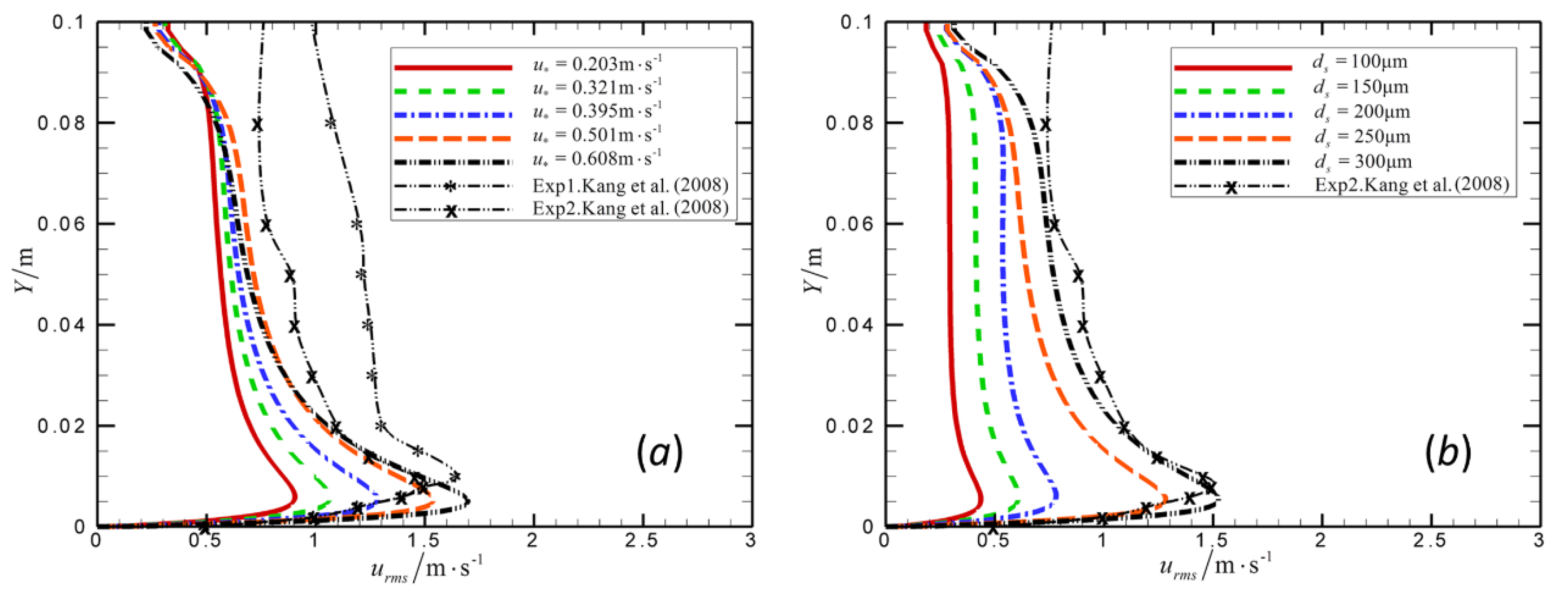
4.4. Fluctuation of the Sand Phase
4.5. Drag between the Two Phases
4.6. Interparticle Collision
5. Conclusions
Author Contributions
Funding
Conflicts of Interest
References
- Bagnold, R.A. The Physics of Blown Sand and Desert Dunes, 1st ed.; Methuen: London, UK, 1954. [Google Scholar]
- Kok, J.F.; Parteli, E.J.R.; Michaels, T.I.; Karam, D.B. The physics of wind-blown sand and dust. Rep. Prog. Phys. 2012, 75, 106901. [Google Scholar] [CrossRef] [PubMed]
- Burr, D.M.; Bridges, N.T.; Marshall, J.R.; Smith, J.K.; White, B.R.; Emery, J.P. Higher-than-predicted saltation threshold wind speeds on Titan. Nature 2015, 517, 60–63. [Google Scholar] [CrossRef] [PubMed]
- Griffin, D.W.; Kellogg, C.A.; Shinn, E.A. Dust in the wind: Long range transport of dust in the atmosphere and its implications for global public and ecosystem health. Glob. Chang. Hum. Health 2001, 2, 20–33. [Google Scholar] [CrossRef]
- Pettke, T.; Halliday, A.N.; Hall, C.M.; Rea, D.K. Dust production and deposition in Asia and the north Pacific Ocean over the past 12 Myr. Earth Planet. Sci. Lett. 2000, 178, 397–413. [Google Scholar] [CrossRef]
- Andreotti, B.; Claudin, P.; Douady, S. Selection of dune shapes and velocities. Part 1: Dynamics of sand, wind and barchans. Eur. Phys. J. B 2002, 28, 321–339. [Google Scholar] [CrossRef]
- Yang, P.; Dong, Z.B.; Qian, G.Q.; Luo, W.Y.; Wang, H.T. Height profile of the mean velocity of an aeolian saltating cloud: Wind tunnel measurements by Particle Image Velocimetry. Geomorphology 2007, 89, 320–334. [Google Scholar] [CrossRef]
- Greeley, R.; Blumberg, D.G.; Williams, S.H. Field measurements of the flux and speed of wind-blown sand. Sedimentology 1996, 43, 41–52. [Google Scholar] [CrossRef]
- Bauer, B.O.; Houser, C.A.; Nickling, W.G. Analysis of velocity profile measurements from wind-tunnel experiments with saltation. Geomorphology 2004, 59, 81–98. [Google Scholar] [CrossRef]
- Creyssels, M.; Dupont, P.; El Moctar, A.O.; Valance, A.; Cantat, I.; Jenkins, J.T.; Pasini, J.M.; Rasmussen, K.R. Saltating particles in a turbulent boundary layer: Experiment and theory. J. Fluid Mech. 2009, 625, 47–74. [Google Scholar] [CrossRef]
- Wang, D.W.; Wang, Y.; Yang, B.; Zhang, W. Statistical analysis of sand grain/bed collision process recorded by high-speed digital camera. Sedimentology 2007, 55, 461–470. [Google Scholar] [CrossRef]
- Zhang, Y.; Wang, Y.; Jia, P. Measuring the kinetic parameters of saltating sand grains using a high-speed digital camera. Sci. China-Phys. Mech. Astron. 2014, 57, 1137–1143. [Google Scholar] [CrossRef]
- Andreotti, B.; Claudin, P.; Douady, S. Selection of dune shapes and velocities. Part 2: A two dimensional modelling. Eur. Phys. J. B 2002, 28, 341–352. [Google Scholar] [CrossRef]
- Haff, P.K.; Anderson, R.S. Particle scale simulations of loose sedimentary beds: The example of particle-bed impacts in aeolian saltation. Sedimentology 1993, 40, 175–198. [Google Scholar] [CrossRef]
- Carneiro, M.V.; Pahtz, T.; Herrmann, H.J. Jump at the onset of saltation. Phys. Rev. Lett. 2011, 107, 098001. [Google Scholar] [CrossRef] [PubMed]
- Chiesa, M.; Mathiesen, V.; Melheim, J.A.; Halvorsen, B. Numerical simulation of particulate flow by the Eulerian-Lagrangian and the Eulerian-Eulerian approach with application to a fluidized bed. Comput. Chem. Eng. 2005, 29, 291–304. [Google Scholar] [CrossRef]
- Mathiesen, V.; Solberg, T.; Hjertager, B.H. An experimental and computational study of multiphase flow behavior in a circulating fluidized bed. Int. J. Multiph. Flow 2000, 26, 387–419. [Google Scholar] [CrossRef]
- Yin, L.J.; Wang, S.Y.; Lu, H.L.; Wang, S.A.; Xu, P.F.; Wei, L.X.; He, Y.R. Flow of gas and particles in a bubbling fluidized bed with a filtered two-fluid model. Chem. Eng. Sci. 2010, 65, 2664–2679. [Google Scholar]
- Pu, W.H.; Zhao, C.S.; Xiong, Y.Q.; Liang, C.; Chen, X.P.; Lu, P.; Fan, C.L. Numerical simulation on dense phase pneumatic conveying of pulverized coal in horizontal pipe at high pressure. Chem. Eng. Sci. 2010, 65, 2500–2512. [Google Scholar] [CrossRef]
- Li, Y.T.; Guo, Y. Numerical simulation of aeolian dusty sand transport in a marginal desert region at the early entrainment stage. Geomorphology 2008, 100, 335–344. [Google Scholar] [CrossRef]
- Durán, O.; Claudin, P.; Andreotti, B. On aeolian transport: Grain-scale interactions, dynamical mechanisms and scaling laws. Aeolian Res. 2011, 3, 243–270. [Google Scholar] [CrossRef]
- Li, Z.Q.; Wang, Y.; Zhang, Y. A numerical study of particle motion and two-phase interaction in aeolian sand transport using a coupled large eddy simulation-discrete element method. Sedimentology 2014, 61, 319–332. [Google Scholar] [CrossRef]
- Smagorinsky, J. General circulation experiments with the primitive equations. I. The basic experiment. Mon. Weather Rev. 1963, 91, 99–164. [Google Scholar] [CrossRef]
- Hu, C.H.; Ohba, M.; Yoshie, R. CFD modelling of unsteady cross ventilation flows using LES. J. Wind Eng. Ind. Aerodyn. 2008, 96, 1692–1706. [Google Scholar] [CrossRef]
- Srivastava, A.; Sundaresan, S. Analysis of a frictional-kinetic model for gas-particle flow. Powder Technol. 2003, 129, 72–85. [Google Scholar] [CrossRef]
- Gidaspow, D. Multiphase Flow and Fluidization: Continuum and Kinetic Theory Descriptions, 1st ed.; Academic Press, Inc.: San Diego, CA, USA, 1994. [Google Scholar]
- Johnson, P.C.; Nott, P.; Jackson, R. Frictional-collisional equations of motion for particulate flows and their application to chutes. J. Fluid Mech. 1990, 210, 501–535. [Google Scholar] [CrossRef]
- Wang, S.Y.; Li, X.; Lu, H.L.; Yu, L.; Sun, D.; He, Y.R.; Ding, Y.L. Numerical simulations of flow behavior of gas and particles in spouted beds using frictional-kinetic stresses model. Powder Technol. 2009, 196, 184–193. [Google Scholar] [CrossRef]
- Johnson, P.C.; Jackson, R. Frictional-collisional constitutive relations for granular materials, with application to plane shearing. J. Fluid Mech. 1987, 176, 67–93. [Google Scholar] [CrossRef]
- Parteli, E.J.R.; Duran, O.; Herrmann, H.J. Minimal size of a barchan dune. Phys. Rev. E 2007, 75, 011301. [Google Scholar] [CrossRef]
- Lun, C.K.K.; Savage, S.B.; Jeffrey, D.J.; Chepurniy, N. Kinetic theories for granular flow–inelastic particles in Couette-flow and slightly inelastic particles in a general flowfield. J. Fluid Mech. 1984, 140, 223–256. [Google Scholar] [CrossRef]
- Sinclair, J.L.; Jackson, R. Gas-particle flow in a vertical pipe with particle-particle interactions. AICHE J. 1989, 35, 1473–1486. [Google Scholar] [CrossRef]
- Schaeffer, D.G. Instability in the evolution equations describing incompressible granular flow. J. Differ. Equ. 1987, 66, 19–50. [Google Scholar] [CrossRef]
- Dupont, S.; Bergametti, G.; Marticorena, B.; Simoens, S. Modeling saltation intermittency. J. Geophys. Res.-Atmos. 2013, 118, 7109–7128. [Google Scholar] [CrossRef]
- Felice, R.D. The voidage function for fluid-particle interaction systems. Int. J. Multiph. Flow 1994, 20, 153–159. [Google Scholar] [CrossRef]
- Kang, L.Q.; Guo, L.J. Eulerian-Lagrangian simulation of aeolian sand transport. Powder Technol. 2006, 162, 111–120. [Google Scholar] [CrossRef]
- Rhie, C.M.; Chow, W.L. A numerical study of the turbulent flow past an isolated airfoil with trailing edge separation. AIAA J. 1983, 21, 1525–1552. [Google Scholar] [CrossRef]
- Leonard, B.P. Order of accuracy of QUICK and related convection-diffusion schemes. Appl. Math. Model. 1995, 19, 640–653. [Google Scholar] [CrossRef]
- Dejoan, A.; Schiestel, R. LES of unsteady turbulence via a one-equation subgrid-scale transport model. Int. J. Heat Fluid Flow. 2002, 23, 398–412. [Google Scholar] [CrossRef]
- Leboreiro, J.; Joseph, G.G.; Hrenya, C.M. Revisiting the standard drag law for bubbling, gas-fluidized beds. Powder Technol. 2008, 183, 385–400. [Google Scholar] [CrossRef]
- Werner, H.; Wengle, H. Large-eddy simulation of turbulent flow over and around a cube in a plate channel. In Proceedings of the The 8th Symposium on Turbulent Shear Flows, Technical University of Munich, Munich, Germany, 9–11 September 1991; Springer: Berlin/Heidelberg, Germany, 1993. [Google Scholar]
- Lu, H.L.; Gidaspow, D. Hydrodynamics of binary fluidization in a riser: CFD simulation using two granular temperatures. Chem. Eng. Sci. 2003, 58, 3777–3792. [Google Scholar]
- Dong, Z.B.; Liu, X.P.; Wang, H.T.L.; Zhao, A.G.; Wang, X.M. The flux profile of a blowing sand cloud: A wind tunnel investigation. Geomorphology 2003, 49, 219–230. [Google Scholar] [CrossRef]
- Dong, Z.B.; Qian, G.Q.; Luo, W.Y.; Wang, H.T. Analysis of the mass flux profiles of an aeolian saltating cloud. J. Geophys. Res.-Atmos 2006, 111, D16111. [Google Scholar] [CrossRef]
- Kang, L.Q.; Guo, L.J.; Gu, Z.M.; Liu, D.Y. Wind tunnel experimental investigation of sand velocity in aeolian sand transport. Geomorphology 2008, 97, 438–450. [Google Scholar] [CrossRef]
- Zhang, W.; Wang, Y.; Lee, S.J. Simultaneous PIV and PTV measurements of wind and sand particle velocities. Exp. Fluids 2008, 45, 241–256. [Google Scholar] [CrossRef]
- Liu, X.P.; Dong, Z. Experimental investigation of the concentration profile of a blowing sand cloud. Geomorphology 2004, 60, 371–381. [Google Scholar] [CrossRef]
- Zhang, W.; Wang, Y.; Lee, S.J. Two-phase measurements of wind and saltating sand in an atmospheric boundary layer. Geomorphology 2007, 88, 109–119. [Google Scholar] [CrossRef]
- Kang, L.Q.; Liu, D.Y. Numerical investigation of particle velocity distributions in aeolian sand transport. Geomorphology 2010, 115, 156–171. [Google Scholar] [CrossRef][Green Version]
- Kang, L.Q.; Zou, X.Y. Theoretical analysis of particle number density in steady aeolian saltation. Geomorphology 2014, 204, 542–552. [Google Scholar] [CrossRef]
- Zheng, Y.; Wan, X.T.; Qian, Z.; Wei, F.; Jin, Y. Numerical simulation of the gas-particle turbulent flow in riser reactor based on k-epsilon-k(p)-epsilon(p)-Theta two-fluid model. Chem. Eng. Sci. 2001, 56, 6813–6822. [Google Scholar] [CrossRef]
- Du, W.; Bao, X.J.; Xu, J.; Wei, W.S. Computational fluid dynamics (CFD) modeling of spouted bed: Influence of frictional stress, maximum packing limit and coefficient of restitution of particles. Chem. Eng. Sci. 2006, 61, 4558–4570. [Google Scholar] [CrossRef]


| Dong et al. (2006) ds = 200–300 μm | Kang et al. (2008) ds = 170–300 μm | Present Simulation ds = 250 μm | |||
|---|---|---|---|---|---|
| u∗ (m/s) | U0 (m/s) | u∗ (m/s) | U0 (m/s) | u∗ (m/s) | U0 (m/s) |
| 0.326 | 8.0 | 0.3525 | 9.3 | 0.203 | 6.5 |
| 0.407 | 10.0 | 0.4131 | 10.9 | 0.321 | 8.5 |
| 0.489 | 12.0 | 0.4397 | 11.6 | 0.395 | 10.5 |
| 0.570 | 14.0 | 0.5117 | 13.5 | 0.501 | 12.5 |
| 0.5382 | 14.2 | 0.608 | 14.5 | ||
| 0.5875 | 15.5 | ||||
© 2020 by the authors. Licensee MDPI, Basel, Switzerland. This article is an open access article distributed under the terms and conditions of the Creative Commons Attribution (CC BY) license (http://creativecommons.org/licenses/by/4.0/).
Share and Cite
Zhang, Y.; Wu, C.; Zhou, X.; Hu, Y.; Wang, Y.; Yang, B. A Numerical Study of Aeolian Sand Particle Flow Incorporating Granular Pseudofluid Optimization and Large Eddy Simulation. Atmosphere 2020, 11, 448. https://doi.org/10.3390/atmos11050448
Zhang Y, Wu C, Zhou X, Hu Y, Wang Y, Yang B. A Numerical Study of Aeolian Sand Particle Flow Incorporating Granular Pseudofluid Optimization and Large Eddy Simulation. Atmosphere. 2020; 11(5):448. https://doi.org/10.3390/atmos11050448
Chicago/Turabian StyleZhang, Yang, Changsong Wu, Xiaosi Zhou, Yuanming Hu, Yuan Wang, and Bin Yang. 2020. "A Numerical Study of Aeolian Sand Particle Flow Incorporating Granular Pseudofluid Optimization and Large Eddy Simulation" Atmosphere 11, no. 5: 448. https://doi.org/10.3390/atmos11050448
APA StyleZhang, Y., Wu, C., Zhou, X., Hu, Y., Wang, Y., & Yang, B. (2020). A Numerical Study of Aeolian Sand Particle Flow Incorporating Granular Pseudofluid Optimization and Large Eddy Simulation. Atmosphere, 11(5), 448. https://doi.org/10.3390/atmos11050448